A Long-Term Ecological Vulnerability Analysis of the Tibetan Region of Natural Conditions and Ecological Protection Programs

Abstract

The combined impacts of drastic natural environment change and increasing human interference are making the uncertainty of the Tibetan Plateau’s ecological vulnerability the world’s largest. In this study, an ecological vulnerability index (EVI) of Tibet in the core area of the Tibetan Plateau was assessed using a selected set of ecological, social, and economic indicators and using a spatial principal component analysis (SPCA) to calculate their weights. The data included Landsat images and socio-economic data from 1990 to 2015 in five-year intervals. The results showed that the total EVI remained at a high vulnerability level, with drastic fluctuation from 1990 to 2000 (a peak in 1995, when there was a sudden increase in light vulnerability, which moved to extreme vulnerability in the next period), and minor fluctuations after 2000, gradually increasing from southeast to northwest. In addition, the spatial analysis showed a distinct positive correlation between the EVI and grassland area (0.33), land use degree (0.15), NDVI (0.14), livestock husbandry output, and a negative correlation in terms of desertification area. The artificial afforestation program (AAP) had a positive significant correlation with NDVI (R² = 0.88), preventing the environment from becoming more vulnerable. The results provide practical information and suggestions for planners to improve the land use degree in urban areas and the vegetation coverage in pastoral regions of the Tibetan Plateau based on the spatial–temporal heterogeneity patterns of the EVI of Tibet.

1. Introduction

The world has been focusing on keeping the ecological ecosystem in a relatively stable dynamic equilibrium state in different aspects, such as the need to balance economic development and ecological conservation [1], and the ecosystem and communities’ response to exterior pressure [2,3]. When the external influences irreversibly exceed the balance range, environmental problems occur worldwide, such as severe climate anomalies [4,5], land desertification [6], ecosystem degradation [7], and natural disasters [8], especially in ecologically vulnerable regions. The potential of an ecosystem’s capability to respond, cope with, and recover when the ecosystem is disturbed by a specific hazard or stressor in a specific time and space is called ecological vulnerability [9,10,11,12,13,14]. Vulnerability includes exposure, sensitivity, and adaptive capacity, which vary according to human interaction with nature. An ecological vulnerability assessment is one of the ways to assess climate change, a highlight in ecological research in recent years [15,16,17]. Therefore, by identifying and targeting vulnerable regions, the threat of intense external forces can be mitigated or prevented, demonstrating the crucial importance of assessing ecological vulnerability for sustainable management and development.

The Intergovernmental Panel on Climate Change (IPCC) presented an effective assessment structure to evaluate ecological vulnerability accurately in 2001 [18]. Ecological vulnerability is considered as the inherent property of the ecosystem to react to hazard sensitivity and its resilience to cope with unexpected pressure [19,20,21]. Furthermore, the methods for assessing ecological vulnerability have been modified based on this structure in the 21st century. Typically, evaluating ecological vulnerability is based on three parts: sensitivity, resilience, and pressure (the PSR model) [22,23,24]. Studies in Europe and coastal areas have mainly focused on the sensitivity of the ecosystem and its response to climate change and pattern change over time [25,26,27,28,29,30], which measure ecosystem tolerance and vegetation response predictions to climate anomalies. In mainland areas, research on ecological vulnerability is more concentrated on land use patterns [31,32,33], desertification soil problems [24,34,35,36], and human disturbances [37,38,39,40,41]. Typically, vulnerable zones with different topological characteristics are studied [38,39,40] to determine the determinants of vulnerability. Appropriate ecological management policy should consider both environmental and socio-economic factors, which are built on an objective and integrated evaluation system. Therefore, a comprehensive ecological vulnerability evaluation system with high accuracy should be applied to these vulnerable areas [41,42,43,44,45]. Scientists have made progress in evaluation methods, including scenario analysis methods [46], quantitative evaluation model methods, and the most widely used, comprehensive index methods. The comprehensive index evaluation system contains selected indicators and the weights of each indicator. The studies predominantly use the analytic hierarchy process (AHP) [24,47,48] and expert scoring [48] to calculate the weight. However, these methods are not just non-objective but also controversial and may not apply to other areas. The analytical unit matters significantly as it displays the accuracy of the study. Yet, currently, most studies use an administration unit instead of a unitive spatial grid unit, resulting in rough conclusions with high inaccuracy and a lack of spatial comparison [49,50,51,52].

As the most fragile and vital region in the world, the Tibetan Plateau, also known as the third pole, has experienced the severe threat of a damaged ecological security barrier and has witnessed serious ecological problems including freeze–thaw erosion [53], hydraulic erosion [54], land desertification [34], grassland degradation [3,55], and salinization [56]. These issues have made the ecosystem difficult to inhabit and maintain a healthy state. The Tibet Autonomous Region is at the margin of the Tibetan Plateau. Approximately 92% of the entire autonomous region lies within the arctic–alpine environment [3] and suffers from frequent crustal movements, drastic wind erosion [8], and freezing erosion [53]. The melting of snow and ice is the fundamental prerequisite for freeze–thaw erosion, and solar radiation is the decisive factor for melting snow and the doubling of the global average in warming speed [51]. Grasslands cover more than 65% of the total Tibet land area [3], and, due to the alpine drought environment, the grassland ecosystem has undergone a significant degradation, leading to decreases in vegetation diversity and productivity [55,57]. Since the grassland ecosystem is irreplaceable for ecological security and pasture output, the inference from climate change and human activities (forage grazing and urbanizing) becomes exceptionally crucial. Hence, the government has implemented several ecological protection projects to increase vegetation coverage in Tibet (

Table 1. Major natural programs on Tibet during 1990–2015 [50,62].

Year of Approval	Name	Scale	Period
1989	Tibet “one river, two rivers” comprehensive development system project	River Basin	1991–2000
1989	Ali Shiquanhe Township Phase I and Phase II Sand Control and Sand Management Project	Prefecture	1992–2000
2002	Grain for Green Program	Region	2002–2020
2005	National Sandy Land Closure Reserve	Region	2005–2020
2005	National Comprehensive Demonstration Area for Sand Control and Prevention	Region	2005–2011
2009	Protection and Construction of Ecological Security Barrier Plan in Tibet	Region	2008–2030
2010	Natural Forest Resources Protection Project in Tibet Autonomous Region	Region	2010–2020
2011	Regional Ecological Construction and Environmental Protection Plan of Qinghai–Tibetan Plateau	Region	2011–2030
2013	Tibet “two rivers four rivers” basin reforestation project planning	River Basin	2014–2030

), and the artificial afforestation program (AAP) is one of the most important and effective means of land greening, especially in arid areas [34,47], which has increased the vegetable coverage rate of Tibet by 16.9% [58].

The AAP is largely implemented in all ecological protection projects listed in Table 1 including country-wide programs such as the Grain for Green Program, the National Comprehensive Demonstration Area for Sand Control and Prevention, and the Closing Hill for Afforestation Program, etc. These listed programs were launched by the Chinese government in the 1980s and have been continuously invested in for the past 25 years [34,47,58]. For instance, the Protection and Construction of Ecological Security Barrier Plan in Tibet, which was conducted by the Chinese government in 2008, had a total investment from the government of 56.66 billion CNY (8.75 billion USD) until 2014 [58]. However, there are still disputes over the use of AAP, as the cost efficiency of AAP is not ideal, and the operation period of AAP exceeds the expectation, which has dismissed the actual needs of local pastoralists [59,60]. Therefore, more investigation on the specific effects and extent of AAP’s influence on reducing ecological vulnerability in Tibet is needed. Mainly, current ecological vulnerability studies in Tibet are limited to specific prefectures or certain aspects of driving factors such as the Sichuan–Tibet railway [37]. These studies have inaccurate analytical units, a small range of study periods, influences from single-type indicators, and inadequate evidence on determinant analysis [40,41,42,43,44,45]. Though numerous studies have investigated ecological health and ecosecurity and assessed the ecological risk of the Tibetan Plateau, more research is still needed on an ecological vulnerability analysis with an ecological protection project policy in the Tibetan Plateau [1,15,31,35,45,49].

In this study, the method was integrated to establish a multiobjective multidimensional ecological vulnerability evaluation system and to analyze the driving factors and relevance between ecological vulnerability and ecological protection project policies. This paper aims to (1) assess EVI in spatial–temporal scale and its determinants in Tibet accurately using spatial principal components analysis (SPCA), (2) identify the relationship between EVI and grasslands and urbanization, (3) validate the impacts that AAP brings to EVI and provide valuable and practical information for planners in environmental policymaking in the Tibetan Plateau.

2. Materials and Methods

2.1. Study Area

Tibet autonomous region (Figure 1), located in western China and the west and south of the Qinghai–Tibetan Plateau (26°50′ N-36°53′ N, 78°25′ E-99°06′ E), accounting for more than half of the area of the Tibetan Plateau and about one-eighth of the total area of China (1.23 × 10⁶ km²), known as the “roof of the world” and the “third pole of the earth”, is the highest altitude place in the world [3]. The region’s topography can be divided into three major areas: the northern Tibetan plateau, the Brahmaputra River basin, and the eastern Tibetan canyon area [57,61]. These regions provide Tibet with abundant natural resources. In these fertile places, the light resources, wind resources, and water resources are the most significant, which are twice than the amount of east coast China in 2016, the average number of windy days per year is up to 100–150 days, with a maximum of up to 200 days, and the largest theoretical reserves of hydro energy resources in China amount to 2.1 × 10⁸ KW, respectively [62,63].

2.2. Assessment and Gradation of Ecological Vulnerability

2.2.1. Evaluation System Framework

The comprehensive ecological vulnerability evaluation system combines the study area’s ecological and socioeconomic conditions in a modified pressure–state–response structure [19,20,21,43,44,45,57,64]. Furthermore, the evaluation index system was constructed by referring to the index system of ecological vulnerability evaluation in the Tibetan highland mountains pre-established by related scholars and expert consultants familiar with the local ecological environment [1,6,15,21,57,62]. The evaluation system is established on the basis of the accessibility and the continuity of the data [64,65,66,67]. The methodological flowchart is shown in Figure 2.

2.2.2. Indicator Selection and Procession

Following the principles of dominant factors, systematicity, and operability [21,22,23,64,65], the multi-index ecological vulnerability evaluation system considered both the objective environment characteristics of Tibet and a comprehensive review of relevant studies [8,15,31,37,49,64,65,67].

As vulnerability is largely interpreted through mountain hazards, grassland degradation, and human activities, variables were chosen with a predisposition to these hazard-affected elements. For example, there are water erosion problems on the southeast edge of Tibet [54] where the environmental factors related to water erosion are topography, vegetation, and precipitation, and the corresponding indicators are slope, vegetation type, vegetation cover, and precipitation. The indices reflected the extent to which these environmental problems affected local ecological vulnerability. The environmental factors related to wind erosion are topography, vegetation condition, and wind speed, and the corresponding indicators are roughness, vegetation cover, and average wind speed.

The evaluation system included 18 variables. These indicators were selected from four major impact factors, which were climate, topography, vegetation, and human disturbance (slope, topographic relief, vegetation coverage, land use degree, landscape diversity, desertification area, plateau permafrost area, grassland area, water resource area, average annual precipitation, relative humidity, average annual temperature, hours of sunshine, wind speed, solar radiation intensity, population density, GDP, and livestock husbandry output). There was information redundancy in these different aspects’ interactions, which was eliminated using a spatial principal components analysis.

This comprehensive ecological vulnerability evaluation system demonstrates the influence of socioeconomic factors on ecological vulnerability, the extent of each indicator, and its relationship with ecological vulnerability.

Considering the influence of different grading schemes on the final vulnerability evaluation results, and the strong subjectivity of grading schemes, to avoid excessive interference of human factors in the process of index grading, this paper adopts the evaluation model of normalized weighted summation of fuzzy classification of indicators for comprehensive research. Continuous data, such as vegetation cover (0, 1), are normalized by the extreme value method, and all indicators with different scales and ranges of values are unified to (0, 1). The effect directions express whether each indicator has a positive or negative relationship with ecological vulnerability. The positive indicator uses the value of the normalization, and the negative indicator is the value of 1 minus the normalization value.

The negative indicators include NDVI, landscape diversity, grassland area, water resource area, average annual precipitation, relative humidity, and average annual temperature. The positive indicators include slope, topographic relief, land use degree, desertification area, plateau permafrost area, hours of sunshine, solar radiation intensity, population density, GDP, and livestock husbandry output. Land use degree represents the proportion of developed land area including built-up area, farmland area, and forest area among the total area in one spatial grid.

Therefore, all indicators are standardized to (0, 1) before the overlay analysis with a 2 km spatial grid evaluation unit [64].

Moreover, in Tibet, the current ecological vulnerability evaluation research is primarily based on the county evaluation unit instead of a uniform spatial grid unit [42], resulting in rough conclusions with high inaccuracy that lack the necessary detailed spatial analysis and localization.

2.2.3. Weight Calculation

Climate, geography, vegetation, social development, and economics are ecological impact elements that may interact in this study’s multi-index integrated ecological vulnerability assessment methodology. Due to the exchanges, there is information redundancy. In the analysis process, this would result in overlapping and redundant information, as well as erroneous and problematic analytical findings [10,11,15,16,21,68,69]. The SPCA technique may successfully maintain relevant primary components by removing information overlap in the original indicator data [12,21,36,43]. The indicators’ weights are determined using SPCA (Spatial Principal Component Analysis) based on PCA (principal component analysis) after the standardization of all indicators in ArcGIS 10.4 [64,65,66,67,68]. Its calculation principle is consistent with PCA, which transforms multiple variables into a few principal components through dimensionality reduction and produces a correlation coefficient matrix composed of each standardized index [10,11,12,44,60,66,67,68,69,70,71,72].

A total of 18 standardized indices were analyzed by principal components analysis to generate 4 new comprehensive indices. In addition, the absolute value of eigenvalue presents the extent of the correlation of indicators and principal components; the more significant the eigenvalue is, the stronger the relationship will be [11,12,17,36,68,72]. The first four principal components whose cumulative contribution rate reached 85% or more were selected; the final principal component result is shown in

Table 2. The results or spatial principal component analysis.

Value	Principal Component	1990a	1995a	2000a	2005a	2010a	2015a
Eigenvalue	I	0.313	0.350	0.342	0.349	0.345	0.340
	II	0.130	0.134	0.134	0.134	0.133	0.135
	III	0.047	0.042	0.037	0.035	0.031	0.032
	IV	0.030	0.031	0.030	0.029	0.029	0.031
Contribution	I	53.079	55.645	55.534	56.659	56.459	55.756
	II	22.087	21.253	21.719	21.705	21.826	22.047
	III	8.014	6.709	6.038	5.679	5.149	5.220
	IV	5.158	4.872	4.893	4.650	4.785	5.071
Cumulative contribution	I	53.079	55.645	55.534	56.659	56.459	55.756
	II	75.166	76.898	77.253	78.365	78.285	77.804
	III	83.180	83.607	83.291	84.044	83.434	83.024
	IV	88.337	88.478	88.184	88.694	88.220	88.095
Weight	I	0.601	0.629	0.630	0.639	0.640	0.633
	II	0.250	0.240	0.246	0.245	0.247	0.250
	III	0.091	0.076	0.068	0.064	0.058	0.059
	IV	0.058	0.055	0.055	0.052	0.054	0.058

(Principal Components I–VI represent the first four principal components among 18 PCs, which were generated by 18 normalized indicators as input layers. Index 1990a–2015a represents the index eigenvalue, contribution, cumulative contribution, and final weight of PC 1–4 each year).

, and the whole contribution of original indexes of ecological vulnerability to principal components is shown in Appendix A,

Table A1. Contribution of original indexes of ecological vulnerability to principal components.

YEAR	PC	Surface Relief Degree	Slope	GDP	Livestock Output	Average Annual Precipitation	Average Annual Temperature	Hours of Sunshine	NDVI	Relative Humidity	Solar Radiation Intensity	Wind Speed	Population Density	Shannon Index	Water Resources Amount	Desertification Area	Grassland Area	Land Use Degree	Plateau Permafrost Area
90	1	0.283	0.283	−0.033	−0.181	0.306	0.306	0.306	0.305	0.090	0.048	−0.253	0.305	0.306	−0.001	−0.093	0.386	0.109	−0.015
90	2	0.153	0.153	0.076	-0.004	0.135	0.135	0.134	0.134	−0.005	0.021	−0.017	0.134	0.134	0.080	0.372	−0.622	−0.546	0.093
90	3	−0.058	−0.058	0.754	0.617	0.056	0.056	0.056	0.058	−0.031	0.045	−0.080	0.059	0.057	−0.030	−0.022	0.109	0.018	0.033
90	4	0.200	0.200	0.078	0.011	0.056	0.056	0.054	0.053	−0.133	-0.005	0.379	0.054	0.056	0.041	−0.535	−0.510	0.427	0.067
95	1	0.273	0.273	0.293	−0.149	0.294	0.294	0.294	0.293	0.119	−0.167	−0.228	0.293	0.294	0.001	−0.077	0.343	0.087	−0.011
95	2	−0.131	−0.131	−0.106	−0.022	−0.107	−0.107	−0.106	−0.106	0.005	0.138	−0.048	−0.106	−0.106	−0.077	−0.374	0.645	0.542	−0.092
95	3	0.098	0.098	0.014	0.536	0.015	0.015	0.014	0.014	−0.028	−0.571	0.567	0.014	0.015	−0.082	−0.067	0.040	0.174	−0.025
95	4	−0.160	−0.160	−0.014	0.419	−0.015	−0.015	−0.014	−0.014	0.173	−0.015	−0.214	−0.014	−0.015	−0.066	0.511	0.525	−0.389	−0.056
00	1	0.277	0.277	0.297	−0.136	0.298	0.298	0.298	0.298	0.125	−0.147	−0.194	0.297	0.298	0.001	−0.076	0.345	0.087	−0.011
00	2	−0.126	−0.126	−0.102	−0.001	−0.103	−0.103	−0.103	−0.103	0.006	0.143	−0.020	−0.103	−0.103	−0.077	−0.375	0.649	0.544	−0.092
00	3	0.040	0.040	-0.007	0.470	−0.007	−0.007	−0.007	−0.007	−0.044	−0.764	0.397	−0.007	−0.007	−0.085	−0.038	0.030	0.148	−0.025
00	4	0.174	0.174	0.023	−0.286	0.025	0.025	0.024	0.024	−0.152	0.051	0.245	0.023	0.025	0.067	−0.546	−0.544	0.404	0.075
05	1	0.273	0.273	0.294	−0.169	0.295	0.295	0.295	0.295	0.113	−0.180	−0.201	0.294	0.295	0.001	−0.075	0.341	0.084	−0.011
05	2	−0.127	−0.127	−0.102	0.016	−0.103	−0.103	−0.102	−0.102	0.022	0.130	−0.033	−0.102	−0.103	−0.077	−0.375	0.652	0.544	−0.092
05	3	0.165	0.165	0.018	0.413	0.020	0.020	0.019	0.019	−0.161	−0.505	0.528	0.018	0.020	−0.066	−0.241	−0.211	0.324	−0.018
05	4	−0.075	−0.075	−0.029	0.443	−0.029	−0.029	−0.029	−0.029	0.120	−0.331	0.029	−0.029	−0.029	−0.134	0.542	0.505	−0.281	−0.127
10	1	0.276	0.276	0.296	−0.105	0.297	0.297	0.297	0.297	0.080	−0.187	−0.224	0.296	0.297	0.001	−0.075	0.339	0.084	−0.010
10	2	−0.123	−0.123	−0.099	0.004	−0.100	−0.100	−0.099	−0.099	-0.001	0.125	−0.001	−0.099	−0.099	−0.078	−0.377	0.655	0.548	−0.093
10	3	0.071	0.071	0.006	0.758	0.007	0.007	0.006	0.006	−0.066	−0.529	0.314	0.007	0.007	−0.050	−0.072	−0.044	0.148	−0.026
10	4	−0.124	−0.124	−0.021	0.302	−0.023	−0.023	−0.022	−0.022	0.128	0.065	−0.151	−0.022	−0.023	−0.071	0.582	0.561	−0.400	−0.111
15	1	0.281	0.281	0.298	−0.124	0.299	0.299	0.299	0.299	0.085	−0.195	−0.181	0.298	0.299	0.000	−0.070	0.336	0.079	−0.010
15	2	−0.112	-0.112	−0.089	0.003	−0.090	−0.090	−0.090	-0.090	0.001	0.121	0.093	−0.090	−0.090	−0.077	−0.380	0.659	0.549	−0.093
15	3	−0.074	−0.074	−0.007	0.837	−0.008	−0.008	−0.008	−0.008	0.019	−0.357	−0.148	−0.006	−0.008	−0.068	0.222	0.263	−0.118	-0.036
15	4	0.117	0.117	0.059	0.367	0.060	0.060	0.059	0.059	−0.161	−0.168	0.346	0.060	0.060	0.093	−0.514	−0.489	0.350	0.071

. The calculation formula was as follows:

$$R=\frac{Z^{T}Z}{n}$$

(1)

$$\left|R-\lambda I\right|=0$$

(2)

$$CCR=\frac{{{\displaystyle \sum }}_{j=1}^m{\lambda }_j}{{{\displaystyle \sum }}_{j=1}^n{\lambda }_j}\ge 0.85$$

(3)

$$P=Z\times W$$

(4)

where R was the correlation coefficient matrix, Z was the standardized value of each selected index, n was the number of indexes, λ was the eigenvalues of the R correlation coefficient matrix, I was the identity matrix, CCR was the cumulative contribution rate, m was the number of principal components that were determined, P was the matrix containing values of every considered principal component, and W was m number of eigenvectors with the largest eigenvalues selected to form the matrix.

2.2.4. EVI Calculation and Gradation

According to the above method, the higher the EVI, the more vulnerable the eco-logical environment. The index is obtained by the sum of the comprehensive values of multiple principal components and their corresponding weights [11,12,36,60,61,62,63,64,68,69,70], as shown in the following formula:

$$EVI={\displaystyle \mathsf{\sum }}_{i=1}^m{r}_m{P}_m$$

(5)

$$r_i=\frac{n_i}{{{\displaystyle \mathsf{\sum }}}_i^m{n}_i}$$

(6)

where EVI is the ecological vulnerability index; r is the contribution ratio; P is the principal component; m is the number of principal components; r_i is the contribution ratio of the i principal component; and n_i is the eigenvalue of the i principal component.

To facilitate spatial analysis, the EVI was classified into five levels using the natural breakpoint classification method (Jenks) in ArcGIS: slight vulnerability: <1.0527, light vulnerability: 1.0527–1.3672, medium vulnerability: 1.3672–1.6817, high vulnerability: 1.6817–2.0676, and extreme vulnerability: >2.0676.

To quantitatively assess the changing trend of the vulnerability of regional eco-systems, a comprehensive regional ecological vulnerability index (EVSI, Ecological Vulnerability Standard Index) needs to be constructed and standardized according to Equation (7) to obtain the comprehensive ecological vulnerability index EVSI of Tibet:

$$EVS{I}_i=\frac{EV{I}_i-EV{I}_{min}}{EV{I}_{max}-EV{I}_{min}}$$

(7)

2.3. Hot Spot Analysis of Ecological Vulnerability

Hot Spot analysis is a spatial analysis model used to display the degree of spatial clustering calculated by Getis-Ord Gi*. The results of the EVI calculations are visualized using the cold/hot spot model. In this study, the Getis-Ord Gi* index was used to analyze the high/low spatial aggregation degree of EVI changes, that is, the spatial distribution of cold/hot spots. Moreover, cold/hot spot analysis is the database that underpins heterogeneity analysis. The calculation formula was:

$$G{i}^{*}=\frac{{{\displaystyle \mathsf{\sum }}}_{j=1}^n{w}_{ij}{x}_j-\overline{X}{{\displaystyle \mathsf{\sum }}}_{j=1}^n{w}_{ij}}{s\sqrt{\left[n{{\displaystyle \mathsf{\sum }}}_{j=1}^n{w}_{ij}^2-{\left({{\displaystyle \mathsf{\sum }}}_{j=1}^n{w}_{ij}\right)}^2\right]/\left(n-1\right)}}$$

(8)

$$\overline{X}=\frac{1}{n}{\displaystyle \mathsf{\sum }}_{j=1}^n{x}_j$$

(9)

$$S=\sqrt{\left(\frac{1}{n}{\displaystyle \mathsf{\sum }}_{j=1}^n{x}_j^2-{\overline{X}}^2\right)}$$

(10)

where Gi* was the output statistical Z-score, x_j was the EVI change of space unit j, and w_ij was the spatial weight between adjacent space units i and j.

2.4. Spatial Correlation Analysis between EVI and Urbanization Index

According to a previous study [13,41], the composite urbanization index (UI) can be quantified through population urbanization, economic urbanization, and land urbanization. These three levels are expressed via population density (PD), GDP density (GDPD), and the area occupied by built-up land (ULP), respectively.

$$UI=\frac{1}{3}\times \left(P{D}^{\prime }+GDP{D}^{\prime }+UL{P}^{\prime }\right)$$

(11)

where UI represents the urbanization index of the evaluation unit and PD′, GDPD′, and ULP′ represent the population density, GDP density, and construction land area ratio of the evaluation unit after standardization.

The spatial correlation between EVSI and UI was analyzed using Moran’s I index. The Monte Carlo test was applied to the analysis 999 times. If Moran’s I > 0, it means that there is a positive correlation between them, and vice versa, there is a negative correlation; additionally, the spatial clustering types of EVSI and UI were obtained in GeoDa software, which were classified as insignificant: high-high, low-low, low-high, and high-low. The formula is as follows:

$$I=\frac{N{{\displaystyle \sum }}_i^N{{\displaystyle \sum }}_{j\ne i}^N{W}_{ij}{Z}_i{Z}_j}{\left(N-1\right){{\displaystyle \sum }}_i^N{{\displaystyle \sum }}_{j\ne i}^N{W}_{ij}}$$

(12)

$$I_{kl}^i=Z_k^i{{\displaystyle \sum }}_{j=1}^N{W}_{ij}{Z}_l^j$$

(13)

$$Z_k^i=\frac{X_k^i-{\overline{X}}_k}{{\sigma }_k}$$

(14)

$$Z_l^j=\frac{X_l^j-{\overline{X}}_l}{{\sigma }_l}$$

(15)

where I is the global bivariate Moran’s I for the EVSI and urbanization and $I_{kl}^i$ is the local bivariate Moran’s I for the EVSI and urbanization level. N stands for the total number of spatial units. $W_{ij}$ stands for spatial weight matrix for measuring the spatial correlation between the i and j spatial units. $Z_i$ refers to the deviation between the attribute of i spatial unit and the average of the attribute. $Z_j$ refers to the deviation between the attribute of j spatial unit and the average of the attribute. $X_k^i$ refers to the value of attribute k of spatial unit i. ${\overline{X}}_k$ refers to the average of attribute k. ${\sigma }_k$ is the variance of attribute k. $X_l^j$ refers to the value of attribute l of spatial unit j. ${\overline{X}}_l$ refers to the average of attribute l. ${\sigma }_l$ refers to the variance of attribute l.

2.5. Correlation between NDVI and Afforestation Area and Regression Tests

The NDVI reflects the absorption and wavelengths characteristics of vegetation in the red and near-infrared regions and, therefore, provides a good indication of ground vegetation growth [73]. The annual and seasonal NDVI averages reflect vegetation growth during the year and season. NDVI is an essential indicator in Tibet, especially when evaluating the grassland growing status and forest conservation [73,74,75]. In addition, the grassland area is the most significant driving factor in ecological vulnerability, according to the result in Section 3.3. Statistical analysis methods must be applied to figure out the effectiveness of AAP policy and the relationship between the effect and EVI. Therefore, NDVI can also reflect the effectiveness of the AAP policy and the correlation between the AAP policy and EVI changing patterns. The NDVI can be the indicator to reflect the extent of the ecosystem coping with the exposure to a hazard [76,77]. However, it is not only determined by the internal resilience of the system, but also by the anthropogenic improvement such as afforestation programs [34,47]. During the study period, some early afforestation area increases was not consistent with NDVI, while the increases in afforestation area alongside decreases in NDVI (especially in 2000, 2005). The regression models in Statistical Product and Service Solutions (SPSS) software were used in this study to analyze the correlation type to explore the relationship between NDVI and afforestation area using the continuous data from 1990 to 2017.

The time series is considered a linear regression function of time: Y = at + b (t stands for the year; where a is the tendency value, a > 0 indicates an increasing trend with time; a < 0 indicates a decreasing trend with time, and the absolute value of a value reflects the rate of increase or decrease.).

2.6. Data Collection

Land use/land cover (LULC), population density (POP), and a digital elevation model (DEM) for 1990, 1995, 2000, 2005, 2010, and 2015 and the normalized difference vegetation index (NDVI) data for 2000–2015 were obtained from the Data Center for Resources and Environmental Sciences, Chinese Academy of Sciences, available online: http://www.resdc.cn (accessed on 27 October 2020). The NDVI data for 1990 and 1995 were obtained from the National Tibetan Plateau Data Center of China, available online: http://data.tpdc.ac.cn/ (accessed on 13 March 2021). The NDVI data were calculated on AVHRR satellite images (the spatial resolution is 1 km). Gross domestic product (GDP) data were obtained from the National Earth System Science Data Sharing Infrastructure, National Science and Technology Infrastructure of China. Meteorological data were provided by the China Meteorological Data Service Center, available online: http://data.cma.cn (accessed on 10 December 2020). Afforestation area data were obtained from the Statistical Yearbook of Tibet in 1990–2018.

3. Results

3.1. Spatial and Temporal Changes of Ecological Vulnerability

The EVI was classified into five levels using the natural breakpoint classification method (Jenks) in ArcGIS (slight vulnerability: <1.0527, light vulnerability: 1.0527–1.3672, medium vulnerability: 1.3672–1.6817, high vulnerability: 1.6817–2.0676, and extreme vulnerability: >2.0676). Throughout the study period, the EVI of Tibet values varied from 0.423 to 2.418, with its highest value in 1995 at 1.925, lowest in 1990 at 1.573, and mean value at 1.774, indicating that Tibet was in a high vulnerability state as a whole.

The proportion of areas with different types of ecological vulnerability for 1990–2015 is shown in Figure 3. On the temporal scale, the light vulnerability area proportion had a short peak in 1995 at 47%, with the most prominent area having an increasing fluctuation of 258.53%. However, the area’s proportion of light vulnerability soon decreased to 9% in 2000. The extreme vulnerability area presented an increasing pattern during the study period and accounted for the most significant area proportion from 2000 onward at around 44%. The area distribution ratio of five ecological vulnerability levels stayed stable in descending order of extreme vulnerability, medium vulnerability, high vulnerability, slight vulnerability, and light vulnerability.

Table 3. The EVI values of all prefectures in Tibet Autonomous Region in 1990–2015.

Year	Lhasa	Qamdo	Shannan	Xigaze	Nagqu	Ngari	Nyingchi	Brahmaputra
1990	1.103	1.296	0.793	1.282	1.862	1.974	0.887	1.103
1995	1.597	1.592	1.255	1.738	2.240	2.254	1.152	1.537
2000	1.461	1.458	1.114	1.594	2.115	2.170	1.001	1.385
2005	1.420	1.380	1.062	1.564	2.088	2.088	0.940	1.346
2010	1.395	1.379	1.045	1.563	2.085	2.140	0.945	1.342
2015	1.456	1.459	1.103	1.584	2.117	2.194	1.010	1.387

shows the percentages of fluctuation of areas with different EVI values per administrative prefecture. The Ngari region was the most vulnerable in all six periods, and Nagqu experienced a peak in 2005 at 2.088, equal to the EVI of Ngari. In 2000, more than half of the prefectures presented an EVI decrease, including Lhasa, Qamdo, Shannan, and Nyingchi (the most significant one). The EVI in 1995 was significantly reduced, and all went through a decline.

The spatial distribution of continuous EVI is shown in Figure 4. Generally, the EVI of Tibet increased primarily in the northern area (mainly in Nagqu and Ngari) over 25 years. Furthermore, the EVI presented a progressively downward trend from north to south. Ecological vulnerability deteriorated considerably in Ngari, Nagqu, and Xigaze. Additionally, the EVI of Ngari stayed in an extremely high status during the study period (high vulnerability in 1990, extreme vulnerability in 1995–2015). Shannan, Lhasa, and Xigaze experienced a significant increase over 25 years, and Xigaze changed from light vulnerability to medium vulnerability. The area of the Brahmaputra River basin had an evident increment in EVI with a spatial pattern of downward trending along the west–east axis, indicating the lower reaches of Brahmaputra River (mainly Nyingchi City) were steadily low vulnerable. The light and slight vulnerability areas were mainly distributed in valley networks and the adret slope of the Transhimalaya and Himalaya, namely, the relatively low-altitude areas.

3.2. Spatial Heterogeneity Analysis of Ecological Vulnerability

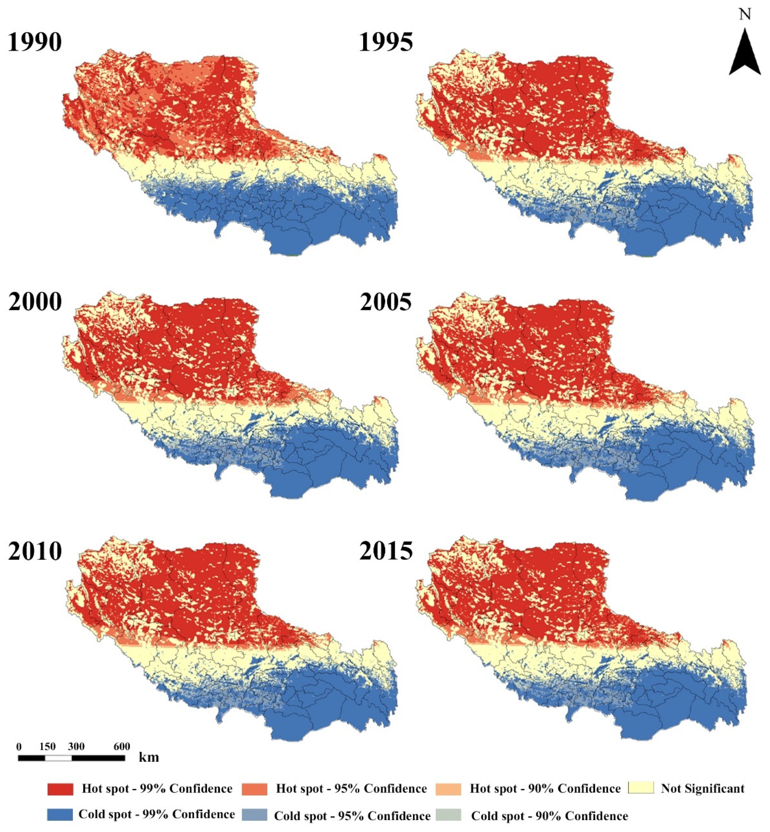
The distribution of cold/hot spots of ecological vulnerability in Tibet during the study period is shown in Figure 5.

Overall, the hot spot was in a stable status with a north to south descending trend. The cold spot generally decreased, mainly in the southern Xigaze, northern Shannan, and Lhasa. The EVI of the whole Nyingchi was in a 99% confidence cold state, indicating that the null hypothesis of complete spatial randomness should be rejected, and this area was 99% expected to present a significant low EVI clustered pattern. Temporal changes demonstrated that the hot spot showed a decreasing trend from 1990 to 2015, with the largest area of hot spots reaching its peak in 1990. The cold spots showed a decreasing–increasing trend from 1990 to 2015, with the largest area of cold spots in 1990. Generally, the hot spot occupied a larger area in Tibet during the study period. Meanwhile, the area of the hot spot and cold spot showed a slight fluctuation after 1995, indicating increasing ecological capacity and stability in cold spot areas.

Regions with significant EVI change filled around 73% of the total Tibet area. Moreover, these regions were mainly located on the edge of Tibet on the north–south axis. Northern Xigaze, Southern Nagqu, and Northern Qamdo showed stable status over 25 years with no significant EVI changes.

Figure 5 shows that the hot spot areas were mainly concentrated in Ngari and Nagqu, and the cold spot areas in Nyingchi, Shannan, and Southern Qamdo. During the study periods, the cold spot in Xigaze, Lhasa, and Shannan was decreased, with an overall EVI increment in these prefectures. In the basin of Brahmaputra, the cold spot area diminished significantly from the middle part to the east part, while the hot spot area stayed unfluctuating.

3.3. Determinant Indicators of EVI

The principal component analysis results are shown in Figure 6. The first four principal component layers, which contributed over 88%, were used to explore the drivers of change in ecological vulnerability in Tibet. Table 1 lists the primary environmental protection programs constructed in Tibet during the study years, which may be relevant to the indices influencing the EVI in Tibet.

In principal component 1 (PC1), the EVI was significantly positively correlated with land use factors such as grassland area (0.3484), NDVI (0.2978), and meteorology factors such as average annual precipitation (0.2983), and average annual temperature (0.2983) from 1990 to 2015. The economic factors are relatively negative with the EVI, with livestock output (−0.1440). Moreover, solar radiation intensity (−0.1379) and wind speed (−0.2135) played the most negative role in 25 years, especially the wind speed factor in 1990 of −0.2530. Since the PC1 accounted for more than half the proportion of the final principal component (55.522%), the indicators that affected the PC1 also played a significant role in the integrated driving factors. Grassland area, average annual precipitation, and average annual temperature were the most vital factors correlated with EVI in Tibet.

PC2, PC3, and PC4 of the EVI were positively correlated with livestock output, land use degree, desertification area, wind speed, and solar radiation intensity, which were quite different from PC1. In general, the grassland area factor remained the most evident one to influence the EVI. The land use degree factor became critical after 1990; the desertification area played an important role, especially in 2010 and 2015. Specifically, GDP was negatively connected to EVI in 1990, while the correlation became diametrically opposite in from 1995 to 2015.

Analysis of the integrated correlation index of PC1-PC4 in 1990–2015 showed that the most influential factor of the EVI was the grassland area, especially in 2005 and 2010. This was followed by land use degree, livestock output, desertification area, and NDVI.

3.4. Effects of Urbanization on EVI

From 1990 to 2015, both the EVI and the urbanization level in Tibet increased significantly, indicating a synergistic change over timescales. The results showed that the EVI and the urbanization level were positively correlated in 1990–2015, and the positive correlation gradually strengthened. The Z-values in

Table 4. Moran’s index and Monte Carlo significance test results of Tibet’s EVI and urbanization levels from 1990 to 2015.

Index	Year	1990	1995	2000	2005	2010	2015
	Moran’s I	0.6352	0.8558	0.8716	0.876	0.8775	0.8781
EVI & Urbanization	|z-Value|	809.3969	1016.2242	979.8041	983.4112	963.4371	1000.1529
	p-Value	0.001	0.001	0.001	0.001	0.001	0.001

(p-values indicate the probability of an event occurring; p < 0.05 indicates a statistically significant difference; and p < 0.01 indicates a statistically significant difference. z-values are multiples of the standard deviation reflecting data dispersion or aggregation, |Z| > 2.58, which corresponds to p < 0.01, indicating a statistically significant difference.).

showed that the EVI and urbanization level had a powerful spatial aggregation effect, with the weakest only in 1990.

Table 5. The urbanization index values of all prefectures in Tibet.

Year	Lhasa	Qamdo	Shannan	Xigaze	Nagqu	Ngari	Nyingchi	Brahmaputra
1990	0.42495	0.38805	0.44562	0.47530	0.55018	0.64446	0.48103	0.46761
1995	0.38228	0.41008	0.27033	0.42695	0.62731	0.66292	0.29619	0.37488
2000	0.38235	0.40997	0.27036	0.42697	0.62726	0.66291	0.29619	0.37479
2005	0.38235	0.40997	0.27036	0.42697	0.62726	0.66291	0.29619	0.37479
2010	0.38279	0.41038	0.27042	0.42731	0.62749	0.66295	0.29631	0.37522
2015	0.38269	0.41029	0.27038	0.42719	0.62740	0.66294	0.29626	0.37509

shows the urbanization index value of all prefectures in Tibet from 1990 to 2015. The indices barely fluctuated in 1995–2015 with a nearly ±0.001 swing. Qamdo, Nagqu, and Ngari were the only prefectures that had grown in urbanization level since 1990. In contrast, Nyingchi had the most significant drop in 1995 from 0.481 (1990) to 0.296 (1995). Table 5 indicates that the urbanization level had spatial heterogeneity, and even though the urbanization level was positively connected to the EVI, the situation was different in each prefecture.

3.5. Correlation between NDVI and Afforestation Area

The interannual trend line equations of the NDVI and afforestation area are listed below in

Table 6. The NDVI and afforestation area inter-annual trend line equation.

Index	Formula	R Square
NDVI	y = 0.0023t − 4.2559	0.9202
Afforestation area	y = 0.0374t − 74.455	0.9283

, indicating that NDVI and afforestation area were positive from 1990 to 2015. Fisher’s test was applied, and the result showed a significant relationship between the NDVI and afforestation area with the R² > 0.85, p < 0.01, and F > 19.00. The standard values of EVI, NDVI, and afforestation area from 1990 to 2015 are shown in Figure 7.

Table 6 and Figure 7 show that the NDVI in Tibet over the 25 years had a positive trend in all, and the afforestation area had an obviously positive trend. This trend means a better turn in the vegetation growth status in afforested areas, and the spatial distribution density also showed an increasing trend in the last 25 years. The negative relevance between the afforestation area and the EVI is shown in Figure 7, indicating that the EVI decreased every five years when the afforestation area increased.

4. Discussion

4.1. The Spatial–Temporal Patterns of Ecological Vulnerability

Overall, the EVI in Tibet has been in a high vulnerability state for 25 years, while extreme vulnerability since 2000 occupied more than 43% of the total study area. The results identified the dynamic patterns in time series and spatial heterogeneity of EVI in Tibet.

In terms of time series, the proportion structure of different ecological vulnerability levels was unstable until 2000. Many high vulnerability areas turned into light vulnerability, and part of them changed into extreme vulnerability. This sudden change in 1995 showed the highest ecological vulnerability value in Tibet at 1.925 throughout the study period. The hot spot analysis showed that in 1995 the count of the not significant area increased and reached a peak (81,153 pixels) with nearly the same amount of cold spot (86,839 pixels), indicating that the increment of ecological vulnerability was mostly spatially random except the north corner of Tibet. Accordingly, the Ngari prefecture and Nagqu prefecture, located in the north part of Tibet, experienced a sharp increase in EVI in 1995. In the meantime, the slightest ecological vulnerability lay in southeastern Tibet, with Nyingchi having the smallest EVI. With Ngari possessing the highest EVI in Tibet from 1990 to 2015, Ngari was considered the most vulnerable region in Tibet, which is in accordance with the hyperaridity, low precipitation, slight hypsography physiognomy topography fluctuation, and severe glacier erosion ecosystems. Moreover, the Ali Shiquanhe Township Phase I and Phase II Sand Control and Sand Management Project was conducted from 1992 to 2000 in Ngari, resulting in urbanization development and relevant construction [78]. At the same time, the construction made the urbanization index increase accordingly (

Table 7. Regression analysis on NDVI and afforestation area.

Formula	R Square	t Stat	p	F	Significance F
y = 0.0042t + 0.2752	0.8777	13.6584	1.89 × 10−38	186.5524	2.2598 × 10−13

) and decrease light vulnerability areas, which made the environment more vulnerable by disarraying resource development.

In the meantime, according to Table 3, southeastern Tibet had a better ecosystem status in comparison to northwestern Tibet, with Shannan and Nyingchi having the least EVI in Tibet during 1990–2015. Though the EVI in southern Tibet rose suddenly in 1995 with the increasing rate of Shannan (58%), Lhasa (45%), Xigaze (36%), it was still less than the northern part and generally stayed in a light vulnerability status. In southeastern Tibet, though the threat of aridity and the significant difference in temperature and elevation, permanent permafrost was diminished, there were also other issues that deteriorated the environment. For instance, abundant forest resources led to over woodcutting and forest damage. Since the timber for the whole of Tibet is mostly taken from southeastern Tibet, this doubled the fall amount in comparison to the growth of forest trees. The situation of unbalanced tree felling brought an increase in the desertification rate and therefore increased the EVI of southern Tibet. There was an evident aggregation in river valleys, low-elevation areas, the adret slope of mountains, and water bodies regarding the slight and light vulnerability area. This clustering certified that protecting these areas is essential. Moreover, the government approved a series of policies to enhance the ecological security barrier of Tibet since 2000, which made the ecosystems in Tibet more stable, yet still fragile. These policies mainly concentrated on solving the desertification issue and improving vegetation cover rate through building conservation areas and expanding the grassland and forest area.

The downstream of the Brahmaputra River basin and open-water bodies were stable and had a low vulnerability, while the upper reaches were the opposite. This consequence means that the Brahmaputra River basin demonstrated a significant spatial variation pattern with EVI descending by the river flow. These findings are consistent with previous research.

Overall, the variation of EVI polarized from 1990 to 2015, with northern Tibet having more fragile in zones with low landscape diversity and arid alpine situations.

4.2. Driving Factors of Ecological Vulnerability

The ecological vulnerability driving factors can be traced back to natural factors and human interferences. As the result of correlation analysis between principal components and various indicators shown in Figure 6, grassland area, land use degree, desertification area, livestock output, and NDVI are the top five critical indicators that affect ecological vulnerability. Solar radiation intensity and wind speed account for the least weight. This proportion indicated that the green vegetation prosperity was the dominant fragment in all factors, followed by the human disturbance indicators (land use degree and livestock output). In comparison, the significance of climate factors and topological factors were relatively inessential.

Among all selected indicators, the influence of the grassland area factor was large not only because the grassland area accounted for the most significant proportion in Tibet, but because of the ecosystem functions of grassland in conserving water and soil, maintaining biodiversity, and controlling wind and sand preventing the environment from becoming more vulnerable [55,57]. The grassland in northwestern Tibet is different from the southeastern. Alpine meadow wetlands form most ecosystems in northwestern Tibet, surrounded by bare lands and glaciers, water bodies, and forests barely distributed there. Therefore, this idiosyncratic landscape pattern may lead to a dramatic response to external interferences and irreversible vulnerability deterioration.

Moreover, as the environment is austere in northwestern Tibet, its population density is relatively low in accordance with an artificial disturbance that placed more responsibilities on the natural aspect resulting in the highest ecological vulnerability index. Meteorological factors including precipitation, relative humidity, temperature, wind speed, and hours of sunshine were the fundamental ingredients affecting the growth of vegetation dynamics [79]. This fact is then related to soil erosion caused by rainfall, wind, and melted snow [80]. Combined soil erosion with topological elements such as elevation and slope can cause brutal geological disasters [81], which further aggravates the vulnerability of the area.

However, the situation is different in southeastern Tibet. Even though the desertification problem still exists here, the cause was not similar to north Tibet. Abundant heat and rainfall along with low elevations and water resources bring south Tibet various landscape patterns and high vegetation coverage. The ecosystem here is far more habitable than in the north, with the essential standards for living guaranteed. Consequently, the urbanization level was lifted by pastoral area intensification and massive project constructions such as the Sichuan–Tibet Railway, diminishing the area of slight and light vulnerability. The disorderly series of constructions raised the urbanization rate of Tibet, according to Table 5. Relatively, EVI was lifted along with the urbanization rate; as a result, Section 3.4 showed a continuous significant positive relation between urbanization rate and EVI. Remarkably, this pattern did not fit every prefecture. In Shannan, the correlation between urbanization and EVI was negative during 1990–2015 [82], which meant that though EVI in Tibet overall was influenced by urbanization, the situation was spatially heterogeneous.

Furthermore, the correlation was gradually strengthened, meaning the influence of urbanization on EVI was fortified and needed more attention to balancing urbanized construction and ecosystem protection. In addition to the disturbance of urbanization, desertification influence was inescapable. The desertification area gradually increased from 1990 to 2015 and was prominently distributed in river valleys and adret regions with lower elevation and closer distance to rivers. This situation appeared in the lower Brahmaputra River basin and valleys resulting from water swilling, geological disasters, and artificial project constructions, especially hydropower projects.

The government has been taking a series of systematic measures to diminish human activities’ influence and prevent natural factors from deteriorating the environment (Table 1). These policies mainly concentrated on increasing vegetation coverage by building or recovering forest and grassland, especially artificial afforestation construction. The positive correlation between the Artificial Afforestation Programme and NDVI to a further extent indicated that AAP raised the vegetation coverage and, therefore, ameliorated the ecosystem status. The improving trend demonstrated critical evidence that with the conduction of AAP, EVI changes and forest areas became better, and this connection strengthened over 25 years, emphasizing the effectiveness of the AAP.

In general, EVI in Tibet is largely influenced by grassland area, and also by land use degree and NDVI. Moreover, land use degree had more significant influence in southeastern Tibet than northwestern Tibet, as the urbanization rate in southeastern Tibet exceeded that of northwestern Tibet.

4.3. Sustainable Implications for Ecosystems Management

The objective reality of Tibet’s fragile ecological environment and the pressure of economic development have made environmental protection in Tibet a severe challenge. As the core variable of environmental change in the Pan-Third Pole, the Tibetan Plateau will pose a significant challenge to the survival and development of more than 20 countries and three billion people in the Pan-Third Pole region if adequate measures are not taken [60]. This study showed that the EVI of Tibet is significantly negatively affected by grassland areas, which are influenced by extreme climate and massive project construction. Therefore, this article offers the following suggestions to prevent the ecological vulnerability of Tibet from increasing further.

Firstly, the grassland ecosystem is susceptible to climate change and grazing. Soil erosion in northern Tibet should be paid attention to in order to take precautions against mountain hazards. These places have been in a highly vulnerable state for 25 years, and even though the government has approved ecological policies to take protection governance, the result still showed a worsening trend. This trend means more powerful and practical measures are needed. Grazing bans and a grass–livestock balance system should be conducted strictly and improving the pasture contract management system can boost the artificial grass planting and natural grassland improvement project and development of shed-feeding and semi-shed-feeding farming. In terms of extreme vulnerability areas in northern and northwestern Tibet, grassland ecological protection subsidy and incentive mechanisms and returning pasture to grass would reinforce the current ecological protection. For southern Tibet, the seriously degraded grasslands need to be fenced off from grazing permanently, and moderately degraded grasslands need to be fenced off from grazing temporarily. Moreover, as the results of artificial afforestation have shown a positive effect on the ecosystem, this policy should be continued and strengthened to accelerate the promotion of sandy land management in middle Tibet and northwest Tibet, and vigorously prevent and control soil erosion in important slight and light vulnerability areas (i.e., water-conserving areas and water and wind erosion staggered areas).

Secondly, from the perspective of optimizing land use degree, pastoral management, refined land function planning, and change of industry structure are needed to solve the aggravated fragmentation of the ecological system. The central conflict here is the need for exploitation and restrictive ecosystem protection. Therefore, in those fenced areas, the primary function can be to plant crops to ensure meeting food demand while the environment is guarded. Moreover, expanding green areas, waters, and wetlands can build a balanced habitable living system as the ecological space is increased. These operational measures can optimize the land use degree and, therefore, improve the ecological vulnerability accordingly.

In summary, the government has implemented a series of environmental protection policies over the past 25 years, and most of them have achieved good results, especially the desertification control along the Brahmaputra River. The government should maintain the above ecological and environmental protection achievements while exploring more effective and appropriate methods for local development.

5. Conclusions

Ecological vulnerability in Tibet varies greatly both temporally and spatially with changes in the natural landscape fragmentation and anthropogenic disturbances such as grazing. This study analyzed the temporal and spatial variation, heterogeneity, driving factors, and the positive aspects that environmental policies have contributed to EVI through a new, integrated evaluation system to quantify ecological vulnerability. The analysis leads to the following conclusions:

(1)

Tibet’s ecological vulnerability level experienced a drastic fluctuation from 1990 to 2000 (peaking in 1995); the proportion pattern stabilized since 2000 with a descending value order as extreme vulnerability (occupied nearly half of Tibet), medium vulnerability, high vulnerability, slight vulnerability, and light vulnerability. In general, Tibet was in a high vulnerability state in the study period. The EVI is more spatially than temporally embodied. The spatial distribution of EVI mainly manifested as a higher vulnerability state in the northwest than that in the southeast with a decreasing trend. In the Brahmaputra River Basin, the EVI increased over 25 years with a descending order, upstream to downstream.

(2)

During the study period, the hot spot center stayed in north Tibet, but the significance of clustering increased; in the meantime, the cold spots clustered in the southeast part of the study area in 1990–2015. The hot spots and the cold spots reached the largest area in 1990, indicating gradual stabilization of the EVI after 1995.

(3)

The EVI determinant factors for Tibet are significantly correlated with grassland area, desertification area, land use degree, and livestock husbandry output and are weakly correlated with the topological indicators. Urbanization level had a crucial positive impact on EVI.

(4)

The Artificial Afforestation Program positively prevents the environment from becoming more vulnerable by increasing NDVI.

This study provides a scientific basis for natural and land use resource development, ecological environment protection, and planning and construction. Therefore, this study can provide policy implementation recommendations for coordinating ecosystem protection and socioeconomic development, helping Tibet to achieve a sustainable state and improve its ecological vulnerability to benefit the Qinghai–Tibet Plateau.

References

1. Dong, H.; Feng, Z.; Yang, Y.; Li, P.; You, Z. Dynamic assessment of ecological sustainability and the associated driving factors in Tibet and its cities. Sci. Total Environ. 2021, 759, 143552. [Google Scholar] [CrossRef]
2. Wang, Y.; Wang, J.; Li, S.; Qin, D. Vulnerability of the Tibetan pastoral systems to climate and global change. Ecol. Soc. 2014, 19, 8. [Google Scholar] [CrossRef] [Green Version]
3. Wang, Y.; Ren, Z.; Ma, P.; Wang, Z.; Niu, D.; Fu, H.; Elser, J.J. Effects of grassland degradation on ecological stoichiometry of soil ecosystems on the Qinghai-Tibet Plateau. Sci. Total Environ. 2020, 722, 137910. [Google Scholar] [CrossRef]
4. Wang, G.; Bai, W.; Li, N.; Hu, H. Climate changes and its impact on tundra ecosystem in Qinghai-Tibet Plateau, China. Clim. Chang. 2011, 106, 463–482. [Google Scholar] [CrossRef]
5. Teng, Y.; Zhan, J.; Liu, W.; Sun, Y.; Agyemang, F.B.; Liang, L.; Li, Z. Spatiotemporal dynamics and drivers of wind erosion on the Qinghai-Tibet Plateau, China. Ecol. Indic. 2021, 123, 107340. [Google Scholar] [CrossRef]
6. Zhan, Q.; Zhao, W.; Yang, M.; Xiong, D. A long-term record (1995–2019) of the dynamics of land desertification in the middle reaches of Yarlung Zangbo River basin derived from Landsat data. Geogr. Sustain. 2021, 2, 12–21. [Google Scholar]
7. Niu, L.; Guo, Y.; Li, Y.; Wang, C.; Hu, Q.; Fan, L.; Wang, L.; Yang, N. Degradation of river ecological quality in Tibet plateau with overgrazing: A quantitative assessment using biotic integrity index improved by random forest. Ecol. Indic. 2021, 120, 106948. [Google Scholar] [CrossRef]
8. Liu, F.; Mao, X.; Zhang, Y.; Chen, Q.; Liu, P.; Zhao, Z. Risk analysis of snow disaster in the pastoral areas of the Qinghai-Tibet Plateau. J. Geogr. Sci. 2014, 24, 411–426. [Google Scholar] [CrossRef]
9. De Lange, H.J.; Sala, S.; Vighi, M.; Faber, J.H. Ecological vulnerability in risk assessment—A review and perspectives. Sci. Total Environ. 2010, 408, 3871–3879. [Google Scholar] [CrossRef]
10. Liu, Y.; Yang, S.; Han, C.; Ni, W.; Zhu, Y. Variability in Regional Ecological Vulnerability: A Case Study of Sichuan Province, China. Int. J. Disaster Risk Sci. 2020, 11, 696–708. [Google Scholar] [CrossRef]
11. Kang, H.; Tao, W.; Chang, Y.; Zhang, Y.; Xuxiang, L.; Chen, P. A feasible method for the division of ecological vulnerability and its driving forces in Southern Shaanxi. J. Clean. Prod. 2018, 205, 619–628. [Google Scholar] [CrossRef]
12. Li, Q.; Shi, X.; Wu, Q. Effects of protection and restoration on reducing ecological vulnerability. Sci. Total. Environ. 2021, 761, 143180. [Google Scholar] [CrossRef] [PubMed]
13. Brunetta, G.; Salata, S. Mapping urban resilience for spatial planning—A first attempt to measure the vulnerability of the system. Sustainability 2019, 11, 2331. [Google Scholar] [CrossRef] [Green Version]
14. Maragno, D.; Pozzer, G.; Musco, F. Multi-Risk Climate Mapping for the Adaptation of the Venice Metropolitan Area. Sustainability 2021, 13, 1334. [Google Scholar] [CrossRef]
15. Li, H.; Song, W. Spatiotemporal Distribution and Influencing Factors of Ecosystem Vulnerability on Qinghai-Tibet Plateau. Int. J. Environ. Res. Public Health 2021, 18, 6508. [Google Scholar] [CrossRef] [PubMed]
16. Liu, Q.; Shi, T. Spatiotemporal differentiation and the factors of ecological vulnerability in the Toutun river basin based on remote sensing data. Sustainability 2019, 11, 4160. [Google Scholar] [CrossRef] [Green Version]
17. Boori, M.S.; Choudhary, K.; Paringer, R.; Kupriyanov, A. Spatiotemporal ecological vulnerability analysis with statistical correlation based on satellite remote sensing in Samara, Russia. J. Environ. Manag. 2021, 285, 112138. [Google Scholar] [CrossRef]
18. Pielke, R.A., Sr. Overlooked issues in the US National Climate and IPCC assessments. Clim. Chang. 2002, 52, 1–11. [Google Scholar]
19. Dossou, J.F.; Li, X.X.; Sadek, M. Hybrid model for ecological vulnerability assessment in Benin. Sci. Rep. 2021, 11, 2449. [Google Scholar] [CrossRef]
20. Sterzel, T.; Lüdeke, M.; Kok, M.; Walther, C.; Sietz, D.; de Soysa, I.; Janssen, P. Armed conflict distribution in global drylands through the lens of a typology of socio-ecological vulnerability. Reg. Environ. Chang. 2014, 14, 1419–1435. [Google Scholar] [CrossRef]
21. Hou, K.; Li, X.; Zhang, J. GIS Analysis of Changes in Ecological Vulnerability Using a SPCA Model in the Loess Plateau of Northern Shaanxi, China. Int. J. Environ. Res. Public Health 2015, 12, 4292–4305. [Google Scholar] [CrossRef] [Green Version]
22. Hu, X.; Ma, C.; Huang, P.; Guo, X. Ecological vulnerability assessment based on AHP-PSR method and analysis of its single parameter sensitivity and spatial autocorrelation for ecological protection—A case of Weifang City, China. Ecol. Indic. 2021, 125, 107464. [Google Scholar] [CrossRef]
23. Xue, L.; Wang, J.; Zhang, L.; Wei, G.; Zhu, B. Spatiotemporal analysis of ecological vulnerability and management in the Tarim River Basin, China. Sci. Total Environ. 2019, 649, 876–888. [Google Scholar] [CrossRef] [PubMed]
24. Wu, C.; Liu, G.; Huang, C.; Liu, Q.; Guan, X. Ecological vulnerability assessment based on fuzzy analytical method and analytic hierarchy process in Yellow River Delta. Int. J. Environ. Res. Public Health 2018, 15, 855. [Google Scholar] [CrossRef] [PubMed] [Green Version]
25. Leclerc, C.; Courchamp, F.; Bellard, C. Future climate change vulnerability of endemic island mammals. Nat. Commun. 2020, 11, 4943. [Google Scholar] [CrossRef]
26. David, C.; Anne, E.-G.; Régis, V.; François, D. A new multimetric index for the evaluation of water ecological quality of French Guiana streams based on benthic diatoms. Ecol. Indic. 2020, 113, 106248. [Google Scholar]
27. Mumini, D.; Danny, S.; Cosmas, M. Assessment of ecological vulnerability to climate variability on coastal fishing communities: A study of Ungwana Bay and Lower Tana Estuary, Kenya. Ocean Coast. Manag. 2018, 163, 437–444. [Google Scholar]
28. Ying, L.; Ge, G.; Lianchun, S. Understanding of Disaster Risk and the Management Associated with Climate Change in IPCC AR5. Adv. Clim. Chang. Res. 2014, 10, 260. [Google Scholar]
29. Bryan, B.; Harvey, N.; Belperio, T.; Bourman, B. Distributed process modeling for regional assessment of coastal vulnerability to sea-level rise. Environ. Modeling Assess. 2001, 6, 57–65. [Google Scholar] [CrossRef]
30. Liquete, C.; Zulian, G.; Delgado, I.; Stips, A.; Maes, J. Assessment of coastal protection as an ecosystem service in Europe. Ecol. Indic. 2013, 30, 205–217. [Google Scholar] [CrossRef] [Green Version]
31. Liu, C.; Li, W.; Zhu, G.; Zhou, H.; Yan, H.; Xue, P. Land Use/Land Cover Changes and Their Driving Factors in the Northeastern Tibetan Plateau Based on Geographical Detectors and Google Earth Engine: A Case Study in Gannan Prefecture. Remote Sens. 2020, 12, 3139. [Google Scholar] [CrossRef]
32. Zhong, L.; Yu, H.; Zeng, Y. Impact of climate change on Tibet tourism based on tourism climate index. J. Geogr. Sci. 2019, 29, 2085–2100. [Google Scholar] [CrossRef] [Green Version]
33. Wang, L.; Wen, C. Traditional villages in forest areas: Exploring the spatiotemporal dynamics of land use and landscape patterns in enshi prefecture, China. Forests 2021, 12, 65. [Google Scholar] [CrossRef]
34. Liu, S.; Zhang, J.; Zhang, J.; Li, Z.; Geng, Y.; Guo, Y. Assessing Controversial Desertification Prevention Policies in Ecologically Fragile and Deeply Impoverished Areas: A Case Study of Marginal Parts of the Taklimakan Desert, China. Land 2021, 10, 641. [Google Scholar] [CrossRef]
35. Li, J.; Yao, Q.; Zhou, N.; Li, F. Modern aeolian desertification on the Tibetan Plateau under climate change. Land Degrad. Dev. 2021, 32, 1908–1916. [Google Scholar] [CrossRef]
36. Li, X.; Song, L.; Xie, Z.; Gao, T.; Wang, T.; Zheng, X.; Liu, J.; Liu, L. Assessment of Ecological Vulnerability on Northern Sand Prevention Belt of China Based on the Ecological Pressure–Sensibility–Resilience Model. Sustainability 2021, 13, 6078. [Google Scholar] [CrossRef]
37. Bao, F.; Qiu, J. Ecological Vulnerability Evaluation Model of Sichuan-Tibet Railway Based on Fuzzy Matter-element Analysis. IOP Conf. Ser. Earth Environ. Sci. 2021, 760, 012029. [Google Scholar] [CrossRef]
38. Yang, H.Z.; Wang, Z.F.; Dai, Q.M. Ecological impact assessment method of highways in Tibetan Plateau: A Case study of Gonghe-Yushu Expressway. J. Mt. Sci. 2020, 17, 1916–1930. [Google Scholar] [CrossRef]
39. Liu, C.; Zhang, F.; Johnson, V.C.; Duan, P. Spatio-temporal variation of oasis landscape pattern in arid area: Human or natural driving? Ecol. Indic. 2021, 125, 107495. [Google Scholar] [CrossRef]
40. Shi, H.; Shi, T.; Liu, Q.; Wang, Z. Ecological Vulnerability of Tourism Scenic Spots: Based on Remote Sensing Ecological Index. Pol. J. Environ. Stud. 2021, 30, 3231–3248. [Google Scholar] [CrossRef]
41. Hong, W.; Jiang, R.; Yang, C.; Zhang, F.; Su, M.; Liao, Q. Establishing an ecological vulnerability assessment indicator system for spatial recognition and management of ecologically vulnerable areas in highly urbanized regions: A case study of Shenzhen, China. Ecol. Indic. 2016, 69, 540–547. [Google Scholar] [CrossRef]
42. Wang, Y.; Ding, Q.; Zhuang, D. An eco-city evaluation method based on spatial analysis technology: A case study of Jiangsu Province, China. Ecol. Indic. 2015, 58, 37–46. [Google Scholar] [CrossRef]
43. Hou, K.; Li, X.; Wang, J.; Zhang, J. An analysis of the impact on land use and ecological vulnerability of the policy of returning farmland to forest in Yan’an, China. Environ. Sci. Pollut. Res. 2016, 23, 4670–4680. [Google Scholar] [CrossRef] [PubMed]
44. Uddin, M.N.; Islam, A.S.; Bala, S.K.; Islam, G.T.; Adhikary, S.; Saha, D.; Haque, S.; Fahad, M.G.R.; Akter, R. Mapping of climate vulnerability of the coastal region of Bangladesh using principal component analysis. Appl. Geogr. 2019, 102, 47–57. [Google Scholar] [CrossRef]
45. Li, H.; Jing, S.; Yang, Z. Ecological vulnerability assessment for ecological conservation and environmental management. J. Environ. Manag. 2018, 206, 1115–1125. [Google Scholar]
46. Yang, Y.; Song, G. Human disturbance changes based on spatiotemporal heterogeneity of regional ecological vulnerability: A case study of Qiqihaer city, northwestern Songnen Plain, China. J. Clean. Prod. 2021, 291, 125262. [Google Scholar] [CrossRef]
47. Li, X.; Zhang, C. Effect of natural and artificial afforestation reclamation on soil properties and vegetation in coastal saline silt soils. Catena 2020. [Google Scholar] [CrossRef]
48. Kumar, M.; Kalra, N.; Singh, H.; Sharma, S.; Rawat, P.S.; Singh, R.K.; Gupta, A.K.; Kumar, P.; Ravindranath, N.H. Indicator-based vulnerability assessment of forest ecosystem in the Indian Western Himalayas: An analytical hierarchy process integrated approach. Ecol. Indic. 2021, 125, 107568. [Google Scholar] [CrossRef]
49. Xia, M.; Jia, K.; Zhao, W.; Liu, S.; Wei, X.; Wang, B. Spatio-temporal changes of ecological vulnerability across the Qinghai-Tibetan Plateau. Ecol. Indic. 2021, 123, 107274. [Google Scholar] [CrossRef]
50. Wei, W.; Shi, S.; Zhang, X.; Zhou, L.; Xie, B.; Zhou, J.; Li, C. Regional-scale assessment of environmental vulnerability in an arid inland basin. Ecol. Indic. 2020, 109, 105792. [Google Scholar] [CrossRef]
51. Jiang, L.; Huang, X.; Wang, F.; Liu, Y.; An, P. Method for evaluating ecological vulnerability under climate change based on remote sensing: A case study. Ecol. Indic. 2018, 85, 479–486. [Google Scholar] [CrossRef]
52. Nguyen, A.K.; Liou, Y.; Li, M.; Tran, T.A. Zoning eco-environmental vulnerability for environmental management and protection. Ecol. Indic. 2016, 69, 100–117. [Google Scholar] [CrossRef]
53. Jiang, X.J.; Zhu, X.; Yuan, Z.Q.; Li, X.G.; Liu, W.; Zakari, S. Lateral flow between bald and vegetation patches induces the degradation of alpine meadow in Qinghai-Tibetan Plateau. Sci. Total Environ. 2021, 751, 142338. [Google Scholar] [CrossRef] [PubMed]
54. Liu, X.; Zhou, Z.; Ding, Y. Vegetation coverage change and erosion types impacts on the water chemistry in western China. Sci. Total Environ. 2021, 772, 145543. [Google Scholar] [CrossRef] [PubMed]
55. Shen, H.; Dong, S.; Di Tommaso, A.; Xiao, J.; Zhi, Y. N deposition may accelerate grassland degradation succession from grasses-and sedges-dominated into forbs-dominated in overgrazed alpine grassland systems on Qinghai-Tibetan Plateau. Ecol. Indic. 2021, 129, 107898. [Google Scholar] [CrossRef]
56. Wang, X.; Li, X.; Cai, D.; Lou, J.; Li, D.; Liu, F. Salinification and salt transports under aeolian processes in potential desertification regions of China. Sci. Total Environ. 2021, 782, 146832. [Google Scholar] [CrossRef]
57. Li, M.; Zhang, X.; He, Y.; Niu, B.; Wu, J. Assessment of the vulnerability of alpine grasslands on the Qinghai-Tibetan Plateau. PeerJ 2020, 8, e8513. [Google Scholar] [CrossRef]
58. China Environmental News. Available online: http://m.haiwainet.cn/middle/455817/2015/0826/content_29100892_1.html (accessed on 26 August 2021).
59. Ma, J.L.; Dong, D.E.H. Closure of mountains for forestry is an effective way to cultivate forests in Sanjiangyuan. In Proceedings of the 2005 CCSA Academic Conference 26 Session (1), Urumqi, China, 20–23 August 2005. [Google Scholar]
60. Yao, G. Analysis of the pros and cons of green forestation on ecological construction. Henan Agric. 2020, 35, 47–48. [Google Scholar]
61. Government of Tibet Autonomous Region. Available online: http://www.xizang.gov.cn/rsxz/ (accessed on 20 May 2021).
62. Yao, T. A comprehensive study of Water-Ecosystem-Human activities reveals unbalancing Asian Water Tower and accompanying potential risks. Chin. Sci. Bull. 2019, 64, 2761–2762. [Google Scholar] [CrossRef] [Green Version]
63. The Tibet Forestry and Grassland Bureau. Available online: http://www.xizang.gov.cn/zwgk/xxfb/ghjh_431/201902/t20190223_61953.html (accessed on 24 September 2021).
64. Guo, B.; Kong, W.H.; Jiang, L.; Fan, Y.W. Analysis of temporal and spatial changes and driving mechanisms of ecosystem vulnerability in the alpine ecological zone of the Qinghai-Tibet Plateau. Ecol. Sci. 2018, 37, 96–106. [Google Scholar]
65. Liou, Y.A. Assessing spatiotemporal eco-environmental vulnerability by Landsat data. Ecol. Indic. 2017, 80, 52–65. [Google Scholar] [CrossRef] [Green Version]
66. Thiault, L.; Marshall, P.; Gelcich, S.; Collin, A.; Chlous, F.; Claudet, J. Space and time matter in social-ecological vulnerability assessments. Mar. Policy 2018, 88, 213–221. [Google Scholar] [CrossRef]
67. Kan, A.K.; Li, G.Q.; Yang, X.; Zeng, Y.L.; Tesren, L.; He, J. Ecological vulnerability analysis of Tibetan towns with tourism-based economy: A case study of the Bayi District. J. Mt. Sci. 2018, 15, 1101–1114. [Google Scholar] [CrossRef]
68. Chang, Y.; Hou, K.; Wu, Y.; Li, X.; Zhang, J. A conceptual framework for establishing the index system of ecological environment evaluation–A case study of the upper Hanjiang River, China. Ecol. Indic. 2019, 107, 105568. [Google Scholar] [CrossRef]
69. Mavhura, E.; Manyangadze, T. A comprehensive spatial analysis of social vulnerability to natural hazards in Zimbabwe: Driving factors and policy implications. Int. J. Disaster Risk Reduct. 2021, 56, 102139. [Google Scholar] [CrossRef]
70. Abson, D.J.; Dougill, A.J.; Stringer, L.C. Using principal component analysis for information-rich socio-ecological vulnerability mapping in Southern Africa. Appl. Geogr. 2012, 35, 515–524. [Google Scholar] [CrossRef]
71. Salata, S.; Grillenzoni, C. A spatial evaluation of multifunctional Ecosystem Service networks using Principal Component Analysis: A case of study in Turin, Italy. Ecol. Indic. 2021, 127, 107758. [Google Scholar] [CrossRef]
72. Demšar, U.; Harris, P.; Brunsdon, C.; Fotheringham, A.S.; McLoone, S. Principal component analysis on spatial data: An overview. Ann. Assoc. Am. Geogr. 2013, 103, 106–128. [Google Scholar] [CrossRef]
73. Jin, J.; Wang, Q. Assessing ecological vulnerability in western China based on Time-Integrated NDVI data. J. Arid Land 2016, 8, 533–545. [Google Scholar] [CrossRef] [Green Version]
74. Liu, Q.; Liu, L.; Zhang, Y.; Wang, Z.; Wu, J.; Li, L.; Li, S.; Paudel, B. Identification of impact factors for differentiated patterns of NDVI change in the headwater source region of Brahmaputra and Indus, Southwestern Tibetan Plateau. Ecol. Indic. 2021, 125, 107604. [Google Scholar] [CrossRef]
75. Liu, Y.; Liu, S.; Sun, Y.; Li, M.; An, Y.; Shi, F. Spatial differentiation of the NPP and NDVI and its influencing factors vary with grassland type on the Qinghai-Tibet Plateau. Environ. Monit. Assess. 2021, 193, 1–21. [Google Scholar] [CrossRef] [PubMed]
76. Yi, Y.; Wang, B.; Shi, M.; Meng, Z.; Zhang, C. Variation in Vegetation and Its Driving Force in the Middle Reaches of the Yangtze River in China. Water 2021, 13, 2036. [Google Scholar] [CrossRef]
77. Hu, T.; Li, X.; Gong, P.; Yu, W.; Huang, X. Evaluating the effect of plain afforestation project and future spatial suitability in Beijing. Sci. China Earth Sci. 2020, 63, 1587–1598. [Google Scholar] [CrossRef]
78. China Forestry News. Available online: http://www.greentimes.com/greentimepaper/html/2019-7/11/content_3334627.htm (accessed on 2 June 2021).
79. Wang, H.; Liu, D.; Lin, H.; Montenegro, A.; Zhu, X. NDVI and vegetation phenology dynamics under the influence of sunshine duration on the Tibetan plateau. Int. J. Climatol. 2015, 35, 687–698. [Google Scholar] [CrossRef]
80. Hoover, D.L.; Knapp, A.K.; Smith, M.D. Resistance and resilience of a grassland ecosystem to climate extremes. Ecology 2014, 95, 2646–2656. [Google Scholar] [CrossRef] [Green Version]
81. Lu, Y.; Zhang, T.; Liu, Y.; You, Y.; Feng, C.; Kong, W. Evaluation and spatial distribution characteristics of freeze-thaw erosion intensity in the Yalu Tsangpo River basin on the basis of geographic information system. Geomat. Nat. Hazards Risk 2019, 10, 1047–1069. [Google Scholar] [CrossRef] [Green Version]
82. Jiang, Y.; Li, R.; Shi, Y.; Guo, L. Natural and Political Determinants of Ecological Vulnerability in the Qinghai–Tibet Plateau: A Case Study of Shannan, China. ISPRS Int. J. Geo-Inf. 2021, 10, 327. [Google Scholar] [CrossRef]
Figure 1. Location of study area.
Sustainability 13 10598 g001
Figure 2. Flowchart of study.
Sustainability 13 10598 g002
Figure 3. The temporal change of five EVI levels proportion from 1990 to 2015 in Tibet.
Sustainability 13 10598 g003
Figure 4. The spatial distribution of EVI in Tibet.
Sustainability 13 10598 g004
Figure 5. Hot spot analysis of EVI.
Sustainability 13 10598 g005
Figure 6. Correlation analysis between principal components 1–4 and various indicators (P–average annual precipitation; T–average annual temperature; Sun–hours of sunshine; POP–population density; LO–livestock husbandry output; S–slope; NDVI; GDP; G–grassland area; PPA–plateau permafrost area; W–wind speed; SRD–surface relief degree; SRI–solar radiation intensity; LUD–land use degree; DA–desertification area; Sh–Shannon index; RH–relative humidity; WRA–water resources amount).
Sustainability 13 10598 g006
Figure 7. Changes in EVI, NDVI, and afforestation area in Tibet from 1990–2015.
Sustainability 13 10598 g007