Evaluation of Five Gas Diffusion Models Used in the Gradient Method for Estimating CO₂ Flux with Changing Soil Properties

Abstract

The gradient method used to estimate soil CO₂ flux is distinctive because it can provide additional information about CO₂ production and consumption of soil profile. However, choosing an appropriate gas diffusion model with confidence with the gradient method is a big challenge. There is no universal optimal diffusion model but only the most suitable model in specific soils. This paper evaluates the applicability of five commonly used diffusion models in laboratory with changing soil properties and in a forest farm, respectively. When soil moisture, bulk density and fertility status were changed in the laboratory, the applicability of the five diffusion models was discussed. Moreover, this paper shows diurnal variation of soil CO₂ flux estimated by the gradient method under four different climatic conditions in the forest farm, and the applicability of the five models was also analyzed. Both laboratory and forest experimental results confirm that the estimating accuracy of the Moldrup model is the highest, followed by the Millington–Quirk model, while those of the Penman, Marshall and Penman–Millington–Quirk models are poor. Furthermore, the results indicate that soil CO₂ flux estimated by the gradient method is highly sensitive to the diffusion model and insensitive to the changes of soil properties. In general, the gradient method can be used as a practical, cost-effective tool to study soil respiration only when the appropriate diffusion model is first determined.

1. Introduction

Soil respiration may constitute up to about three-quarters of total ecosystem respiration, which has an important impact on the global carbon cycle and climate change [1,2]. Therefore, soil carbon dioxide (CO₂) emissions have received much attention [3,4]. Currently, the most widely used soil CO₂ flux measuring methods are the micro-meteorological eddy covariance method [5,6,7], the chamber method [8,9,10] and the gradient method [11,12,13]. However, both the eddy covariance method and the chamber method only measure the accumulation of CO₂ released from soil surface, while the gradient method can provide additional information about soil depth profile, which is vital for understanding the mechanisms of CO₂ production or consumption at certain soil depths.

The gradient method uses Fick’s first law to estimate soil CO₂ flux based on CO₂ concentration in the vertical soil profile and the CO₂ diffusion coefficient in the soil (D_S) [11,14]. It is important to note that D_S is the most crucial parameter for the calculation of soil CO₂ flux and determining D_S with confidence is a big challenge. D_S depends on the soil properties, such as total soil porosity and air-filled porosity. Since it is difficult to measure D_S directly in situ, the most common approach to determine D_S is to employ gas diffusion models [15,16]. Currently, there are many different diffusion models used in the D_S calculation, including single parameter models with soil porosity as the only parameter and complex parameter models with total soil porosity and air-filled porosity [17,18]. Choosing a diffusion model must be considered carefully because the estimation of CO₂ flux is directly affected. It is very important to understand that, besides some common factors such as soil temperature, moisture, bulk density, organic matter, water table, etc., the most suitable model would also depend on some occasional factors. Therefore, there is no universal optimal D_S model for all soil types but only the most suitable model for the respective soil.

Many researchers selected one D_S model when using the gradient method to estimate soil CO₂ flux, but there was little explanation why they chose that diffusion model rather than other models [19,20,21,22]. Tang et al. (2003) [19] assessed soil respiration in a Mediterranean savanna ecosystem using the gradient method. Based on the soil CO₂ gradient and the diffusion coefficient calculated by the Millington–Quirk model (1961), the estimated soil CO₂ flux using the gradient method was close to the chamber measurements. Riveros-Iregui et al. (2008) [20] presented measurements of soil CO₂ flux in a characteristic subalpine forest of the northern Rocky Mountains. The Moldrup model (1999) was selected to calculate diffusion coefficient using the gradient method, and there was a good agreement with the measurements by the chamber method. It can be noticed that researchers usually indicated which diffusion model to use directly in the literature, but the reason for choosing the D_S model was not elaborated and the error range caused by selecting other diffusion models was not analyzed. Pingintha et al. (2010) [23] compared six common diffusion models used in the gradient method to estimate soil CO₂ flux, and they found that the Moldrup model (1997) yielded soil CO₂ flux closest to the results of the chamber method. Moreover, they pointed out that the Moldrup model (1997) was a general model independent of soil type, but did not verify the applicability of this model in different soil types.

In addition, previous studies have indicated that soil CO₂ flux is greatly affected by soil properties, especially soil temperature and moisture [19,24]. It has been acknowledged that soil CO₂ flux correlated exponentially with soil temperature, and the relationship with soil moisture remains to be explored [25]. However, few researchers have reported the effects of soil bulk density and fertility status on soil CO₂ flux. Certainly, the applicability of the diffusion models needs to be further determined when soil properties change.

In order to bolster our confidence in using the gradient method to estimate soil CO₂ flux, this study evaluates the applicability of five commonly used D_S models in the laboratory with changing soil properties (moisture, bulk density, and fertility status) and in a forest farm with four different climatic conditions, respectively. Meanwhile, the effects of soil moisture, bulk density and fertility status on soil CO₂ flux were analyzed. The alkali absorption and chamber method were separately used as references to evaluate the applicability of diffusion models in the laboratory and the forest farm.

2. Materials and Methods

2.1. The Gradient Method

The soil CO₂ flux ($F$, μmol·m⁻² s⁻¹) can be determined by Fick’s first law [11]

$$F=-D_S\frac{\Delta C\left(z\right)}{\Delta z}$$

(1)

where C is the CO₂ concentration (μmol·m⁻³) at the soil depth z(m), and D_S is the CO₂ diffusion coefficient in the soil (m² s⁻¹). The negative sign indicates that the flux is in the reverse direction of the concentration gradient. D_S can be estimated as

$$D_S=\xi D_a$$

(2)

where $\xi$ is the relative gas diffusion coefficient, and $D_a$ is the CO₂ diffusion coefficient in the free air. The influence of temperature and pressure on $D_a$ is given by

$$D_a=D_{a0}\times {\left(\frac{T}{T_0}\right)}^{1.75}\times \frac{P_0}{P_a}$$

(3)

where T is the temperature (K), $P_0$ is the air pressure (Pa) and $D_{a0}$ is a reference value of $D_a$ at $T_0$ (293.15 K) and $P_a$ (101.3 kPa), given as 1.47 × 10⁻⁵ m² s⁻¹ [26]. There are many empirical models to calculate $\xi$, and the applicability of five common models was assessed in this study.

The Millington–Quirk (MQ) model [27] was presented as

$$\xi =\frac{{\alpha }^{\frac{10}{3}}}{{\varphi }^2}$$

(4)

The Penman model [28] was shown as

$$\xi =0.66\alpha$$

(5)

The Marshall model [29] was expressed as

$$\xi ={\alpha }^{1.5}$$

(6)

The Penman–Millington–Quirk (PMQ) model [30] was described as

$$\xi =0.66\alpha \times {\left(\frac{\alpha }{\varphi }\right)}^{\frac{12-m}{3}}$$

(7)

The Moldrup model [31] was proposed as

$$\xi =\frac{{\alpha }^{2.5}}{\varphi }$$

(8)

where $\varphi$ is the total soil porosity (cm³ cm⁻³),$\alpha$ is the air-filled porosity in the soil (cm³ c m⁻³); the value of m in the PMQ model is 3. The relationship between $\varphi$ and $\alpha$ is

$$\varphi =1-\frac{{\rho }_b}{{\rho }_m}$$

(9)

$$\alpha =\varphi -{\theta }_v$$

(10)

where ${\theta }_v$ is the soil volumetric water content (cm³ cm⁻³), ${\rho }_b$ is the soil bulk density (g·cm⁻³) and ${\rho }_m$ is the particle density of mineral soil with a typical value of 2.65 g·cm⁻³.

2.2. Soil CO₂ Concentration, Moisture and Temperature Measurements

Figure 1 shows that CO₂ concentration, moisture and temperature were simultaneously measured at soil vertical depths of 3 cm, 10 cm and 18 cm, respectively. Three CO₂ sensors (T6615, Amphenol Corporation, Boston, MA, USA), based on non-dispersive infra-red (NDIR) technique, were used for soil CO₂ concentration measurements with a range of 0–10,000 ppm. The accuracy of T6615 is 75 ppm or 10% of the reading (whichever is greater). In addition, T6615 is a low-power sensor and consumes less than 0.9 W, which can minimize heating the soil and avoid changing the soil microclimate. As shown in Figure 2, the CO₂ probe was developed by sealing T6615 in a polyvinyl chloride (PVC) cylinder (length = 13 cm, diameter = 5.5 cm), and the upper and lower ends were sealed with rubber gaskets. Eight round drilling holes (diameter = 6 mm) on the CO₂ probe were separately covered with the membranes (diameter = 16 mm) made of sintered PTFE (polytetrafluoroethylene), which could protect the probe from water and ensure gas exchange between the probe and the soil. Moreover, we used a thermal resistance sensor PT100 to measure soil temperature, and self-developed moisture sensors (HYSWR-ARC) to monitor soil moisture [32]. Temperature and moisture sensors were installed at the same depth where the CO₂ probes were buried. Soil CO₂ concentration, temperature and moisture profile measurements were recorded every half-hour with a data logger (CR23x, Campbell Scientific Inc., Logan, UT, USA).

2.3. Laboratory Experiment

2.3.1. A General Description of the Laboratory Experiment

Soil samples with five levels of moisture, three different bulk densities and four fertility conditions were prepared in the laboratory. Soil CO₂ flux was estimated by using the MQ, Penman, Marshall, PMQ and Moldrup models, respectively. Meanwhile, the alkali absorption method was employed as a reference to assess the applicability of the five diffusion models. As shown in Figure 3, an Erlenmeyer flask containing 10 mL of NaOH solution (1 mol/L) was placed in the airtight PVC chamber, which was taken out after 24 h and excess BaCl₂ was dropped in. Phenolphthalein was used as an indicator and 1 mol/L standard hydrochloric acid for titration to calculate the soil CO₂ flux within a 24 h period [33]. Three tests were replicated at each level of soil moisture, bulk density and fertility status.

2.3.2. Sampling Site

Soil samples were collected from Jiufeng National Forest Park (39°54′ N, 116°28′ E), Beijing, China. The climate of this park is a typical warm-temperate continental climate with a mean annual temperature of 11.6 °C and a mean annual precipitation of 600 mm [34]. The sampling position is located in a homogeneous forest where Quercusvariabilis is the dominant species.

2.3.3. Soil Samples Preparation

The retrieved soils were oven-dried for 24 h at 105 °C, and then passed through a 2 mm sieve. Soil samples with five levels of moisture ranging from dry to near saturation were prepared. The oven-dried soils were equally divided into five parts and re-moistened with 0.5 kg, 1 kg, 1.5 kg, 2 kg and 2.5 kg water, respectively. Then they were uniformly packed into cylinders with 25 cm in diameter and 46 cm in height, and the bulk density ${\rho }_b$ is controlled at 1.16 ± 0.02 g·cm⁻³.

Soil samples with three different bulk densities were conducted using a procedure similar to the Proctor compaction test described by Ayers and Perumpral (1982) [35]. A PVC cylindrical mold (diameter = 25 cm, height = 46 cm) was used to pack the sample with a PVC rod (diameter = 5 cm, length = 48 cm, weight = 1 kg) as the drop hammer. Compaction was carried out by dropping the hammer at a constant height of 20 cm as soil was placed into the mold in layers [36]. The three different bulk densities of soil samples were procured by 3, 8 and 15 blows per layer, respectively.

Soil samples with four fertility conditions were prepared by adding nitrogen (N) fertilizer, phosphorus (P) fertilizer, potassium (K) fertilizer and organic fertilizer (fermented chicken manure), respectively. The oven-dried soils were equally divided into five parts, one of which was mixed with 1 kg water as a control, and others were separately mixed with 1 kg solutions of N fertilizer, P fertilizer, K fertilizer and organic fertilizer. Then they were uniformly packed into cylinders (diameter = 25 cm, height = 46 cm), and all of these five soil samples have the same water content (θ_v = 13.1 ± 0.3%) and a uniform bulk density (ρ_b = 1.12 ± 0.06 g·cm⁻³).

2.4. Forest Experiment

2.4.1. Site Description

The forest experiment was conducted in Gongqing Forest Park (40° 06′ N, 116° 42′ E), Beijing, China, which is located in warm temperate zone with continental monsoon climate. The mean annual air temperature is about 13.4 °C, and the average annual precipitation is about 571 mm [37]. This study was carried out in a homogeneous forest area where poplar is the dominant species and the soil texture is 92% sand, 2% silt and 6% clay. The ground water table level was around 2 m, with seasonal fluctuation of about ±0.5 m. The water table may be the dominant or strongest control alone or together with soil temperature according to the previous studes [38,39,40,41]. In this study, the effect of water table on respiration can be reflected by soil moisture.

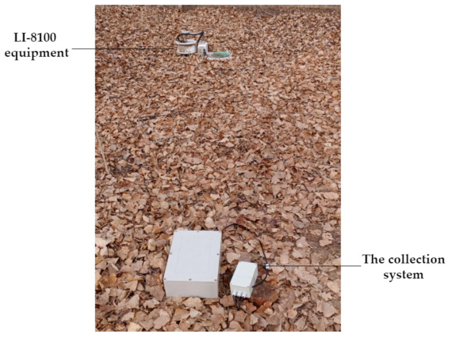
2.4.2. Field Measurements

The CO₂ probes, moisture and temperature sensors were separately installed at the same soil vertical depths of 3 cm, 10 cm and 18 cm. They were located two meters away from a soil respiration chamber (LI-8100, LI-COR Inc., Lincoln, NE, USA) (Figure 4). Moreover, soil bulk density was determined by classical cylinder core sampling method. CO₂ flux was estimated by the gradient method using the MQ, Penman, Marshall, PMQ and Moldrup models respectively. To assess the applicability of these diffusion models, soil CO₂ fluxes estimated from the gradient method were compared with the measurements of LI-8100 chamber.

The measuring system was installed and tested on 30 September 2019. In order to avoid the influence of soil disturbance on the measurements, we collected the measuring data after 8 May 2020 as the soil environment had time to settle.

3. Results and Discussion

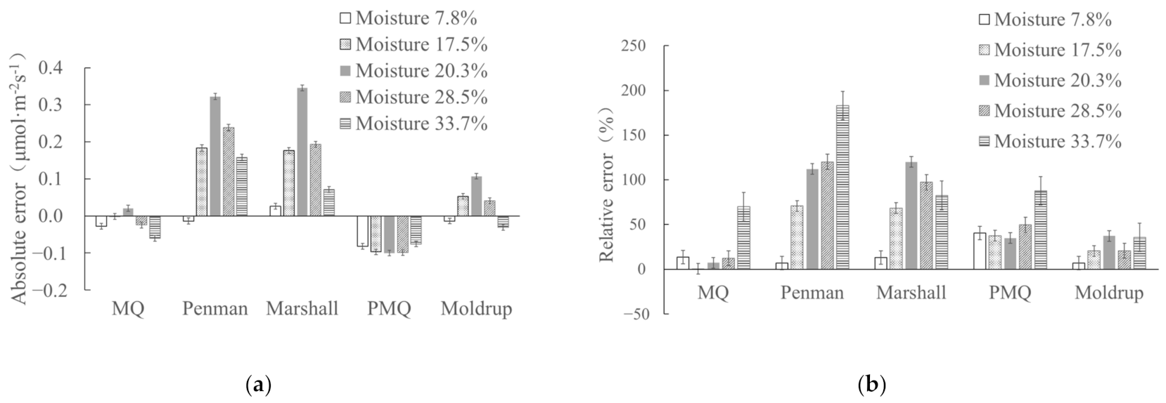
3.1. Effect of Soil Moisture on Applicability of Diffusion Models

The averaged CO₂ fluxes of soil samples were measured by the alkali absorption method and the gradient method in the laboratory for 24 h. Fick’s first law was used to estimate CO₂ fluxes of soil samples with five moisture levels ranging from dry to near saturation. The MQ, Penman, Marshall, PMQ and Moldrup models were used to calculate the relative gas diffusion coefficient ξ, respectively.

As shown in

Table 1. Soil CO₂ flux measured at different water contents (T = 23 °C, ρ_b = 1.16 ± 0.02 g·cm⁻³).

θv (%)	F (μmol·m−2 s−1)
	Alkali Absorption Method	MQ Model	Penman Model	Marshall Model	PMQ Model	Moldrup Model
7.8	0.202 ± 0.008	0.174 ± 0.008	0.188 ± 0.009	0.228 ± 0.009	0.119 ± 0.007	0.188 ± 0.008
17.5	0.288 ± 0.009	0.258 ± 0.009	0.443 ± 0.010	0.436 ± 0.010	0.162 ± 0.012	0.312 ± 0.009
20.3	0.295 ± 0.009	0.309 ± 0.009	0.610 ± 0.011	0.633 ± 0.011	0.188 ± 0.008	0.395 ± 0.007
28.5	0.199 ± 0.008	0.174 ± 0.008	0.437 ± 0.010	0.392 ± 0.009	0.100 ± 0.008	0.240 ± 0.008
33.7	0.086 ± 0.008	0.026 ± 0.007	0.244 ± 0.009	0.158 ± 0.008	0.011 ± 0.010	0.056 ± 0.009

, when the soil moisture increased from dry (θ_v = 7.8%) to near saturation (θ_v = 33.7%) gradually, the CO₂ flux also increased and reached the peak value as θ_v is 20.3%, and then decreased to the minimum value as θ_v is 33.7%. The results of the alkali absorption method and the gradient method were consistent. It is obvious that soil CO₂ flux is sensitive to soil moisture. When soil moisture is low, the respiration of microorganisms in soil is weak, and CO₂ production rates are limited. When soil moisture gradually increases, the activities of microorganisms in soil are stronger, and then soil CO₂ flux increases. Similar results have been reported by some previous studies [18,23,42,43]. The reason for the decreased soil CO₂ flux under high moisture is that the gas transport in soil is limited because soil porosity is mainly filled by liquid water.

Figure 5 shows the absolute and relative errors between the CO₂ flux separately calculated by the five diffusion models and the results of the alkali absorption method under different soil moisture contents. When the soil volumetric moisture content was 7.8%, the mean absolute errors of the MQ, Penman, Marshall, PMQ and Moldrup models were 0.028, 0.014, 0.026, 0.082 and 0.014 μmol·m⁻² s⁻¹ respectively, and the mean relative errors were 13.64%, 6.86%, 13.09%, 40.61% and 6.75% respectively. With the increase of soil moisture, the absolute and relative errors of the Penman, Marshall and PMQ models increased significantly, and the stabilities of the three models were weak. The absolute errors of the MQ and Moldrup models are both less than 0.1 μmol·m⁻² s⁻¹. In general, the error value of the Moldrup model is slightly larger than that of the MQ model, while the relative error of the MQ model is larger when the soil moisture content is close to saturation. Therefore, when the soil moisture in this study varied from low (θ_v = 7.8%) to near saturation (θ_v = 33.7%), the MQ and Moldrup models had better applicability in calculating soil CO₂ flux.

3.2. Effect of Soil Bulk Density on Applicability of Diffusion Models

The averaged CO₂ fluxes were measured by the alkali absorption method and the gradient method in the laboratory for 24 h. Bulk densities of the three soil samples were 1.02, 1.19 and 1.34 g·cm⁻³, and the moisture content of each soil sample was the same (θ_v = 10.2%). The MQ, Penman, Marshall, PMQ and Moldrup models were used to calculate ξ, respectively.

Table 2. Soil CO₂ flux F (μmol·m⁻² s⁻¹) measured under different bulk densities (T = 23 °C, θ_v = 10.2%).

Bulk Density (g·cm−3)	F (μmol·m−2 s−1)
	Alkali Absorption Method	MQ Model	Penman Model	Marshall Model	PMQ Model	Moldrup Model
1.02	0.115 ± 0.007	0.119 ± 0.007	0.170 ± 0.008	0.169 ± 0.008	0.082 ± 0.008	0.133 ± 0.007
1.19	0.144 ± 0.008	0.130 ± 0.007	0.193 ± 0.008	0.188 ± 0.008	0.090 ± 0.008	0.145 ± 0.008
1.34	0.173 ± 0.008	0.152 ± 0.008	0.256 ± 0.009	0.157 ± 0.008	0.103 ± 0.008	0.175 ± 0.008

shows that soil CO₂ flux can be affected by bulk density. When bulk density increased, the porosity of the soil would decrease, and the diffusion coefficient D_S decreased accordingly. However, the increase of the CO₂ concentration difference in the soil profile was greater than the decrease of the gas diffusion coefficient, which caused the increase of soil CO₂ flux. This result is in accordance with the previous study. Our data also support the hypothesis by Moldrup et al. (2001) [44] and (2003) [45] that local-scale variations in soil bulk density may be a controlling factor for gas diffusivity in undisturbed soil and may partly explain why measured gas diffusivities in undisturbed soil are often lower than in repacked soil at the same air-filled porosity.

Figure 6 shows the absolute and relative errors between the CO₂ flux separately calculated by the five diffusion models and the results of the alkali absorption method under different bulk densities. It can be seen that the calculation results of the Penman, Marshall and PMQ models have large errors with the measurement results of the alkali absorption method. When the soil is relatively loose, the mean absolute errors of the CO₂ flux calculated by the MQ and Moldrup models are 0.004 and 0.002 μmol·m⁻² s⁻¹ respectively, and the relative errors are 3.68% and 15.20%, respectively, implying that the MQ model is slightly better than the Moldrup model. However, when the soil bulk densities increase to 1.19 and 1.34 g·cm⁻³, the mean absolute errors of the MQ model are 0.014 and 0.021 μmol·m⁻² s⁻¹, respectively, and the mean absolute errors of the Moldrup model are 0.001 and 0.002 μmol·m⁻² s⁻¹, respectively, implying that the Moldrup model performs better than the MQ model. Therefore, the Moldrup model has the best applicability when calculating soil CO₂ flux under different bulk densities, followed by the MQ model, while the Penman, Marshall and PMQ models have poor applicability.

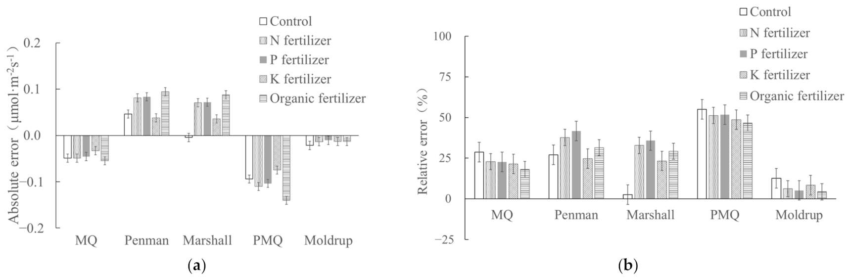
3.3. Effect of Soil Fertility on Applicability of Diffusion Models

CO₂ fluxes of soil samples with five different fertility statuses were evaluated in the laboratory. The five samples were prepared by soil without fertilization (as a control), soil with N fertilizer, P fertilizer, K fertilizer and organic fertilizer (fermented chicken manure), respectively. The MQ, Penman, Marshall, PMQ and Moldrup models were used to calculate ξ, respectively.

As shown in

Table 3. Soil CO₂ flux measured at different fertility status (T = 23 °C, θ_v = 13.1 ± 0.3%, ${\rho }_b$= 1.12 ± 0.06 g·cm⁻³).

Fertility Status	F (μmol·m−2 s−1)
	Alkali Absorption Method	MQ Model	Penman Model	Marshall Model	PMQ Model	Moldrup Model
Control	0.171 ± 0.005	0.139 ± 0.007	0.224 ± 0.008	0.222 ± 0.008	0.090 ± 0.008	0.163 ± 0.008
N fertilizer	0.215 ± 0.008	0.187 ± 0.008	0.305 ± 0.009	0.299 ± 0.011	0.122 ± 0.009	0.220 ± 0.006
P fertilizer	0.201 ± 0.006	0.177 ± 0.008	0.293 ± 0.010	0.286 ± 0.009	0.114 ± 0.007	0.209 ± 0.008
K fertilizer	0.154 ± 0.008	0.121 ± 0.007	0.192 ± 0.008	0.190 ± 0.008	0.079 ± 0.008	0.141 ± 0.007
Organic fertilizer	0.301 ± 0.007	0.246 ± 0.009	0.395 ± 0.009	0.389 ± 0.009	0.161 ± 0.011	0.288 ± 0.009

, soil CO₂ flux decreased slightly after adding K fertilizer, and increased after addition of N fertilizer, P fertilizer and organic fertilizer. It was obvious that the impact of the organic fertilizer on soil respiration was the greatest, and the effects of P fertilizer and K fertilizer were not significant. The results of the alkali absorption method and the gradient method were consistent.

Figure 7 shows the absolute and relative errors between the CO₂ flux separately calculated by the five diffusion models and the results of the alkali absorption method under different fertility status. It can be seen that the calculation results of the Penman, Marshall and PMQ models have large errors with the measurement results of the alkali absorption method, while the errors of the MQ and Moldrup models are smaller. The mean absolute error of the control sample and the samples adding N, P, K and organic fertilizer calculated by the MQ model were 0.049, 0.049, 0.045, 0.033 and 0.054 μmol·m⁻² s⁻¹, and the mean relative errors were 28.72%, 22.88%, 22.68%, 21.46% and 18.13%, respectively. The mean absolute errors calculated by the Moldrup model were 0.022, 0.013, 0.010, 0.013 and 0.013 μmol·m⁻² s⁻¹, and the mean relative errors were 12.61%, 6.19%, 5.18%, 8.44% and 4.32%, respectively. In general, the error value of the MQ model is slightly larger than that of the Moldrup model. Therefore, the Moldrup model has the best applicability when calculating soil CO₂ flux under different fertility status, followed by the MQ model, while the Penman, Marshall and PMQ models have poor applicability.

3.4. Correlation Analysis between the Five Model Calculations and the Measurements

To comprehensively address the relationship between the five model calculations and the measurements of alkali absorption method in detail,

Table 4. The relationship between the five model calculations and the measurments of alkali absorption method (F = a × x; F represents the calculation of each model, and x represents the measuremment of alkali absorption method).

Method	F (μmol·m−2 s−1)			Parameter
	Maximum	Minimum	Average	Slope (a)	R2
MQ model	0.309	0.026	0.170	0.884	0.986
Penman model	0.610	0.170	0.304	1.550	0.944
Marshall model	0.633	0.157	0.288	1.504	0.947
PMQ model	0.188	0.011	0.109	0.566	0.985
Moldrup model	0.395	0.056	0.205	1.067	0.982
Alkali absorption	0.301	0.086	0.196

shows the correlation analysis between the calculations and the measurements. It can be seen from the results that the slope of the Moldrup model is closest to 1 (1.067, slight overestimation), followed by the Millington–Quirk model (0.884, slight underestimation). However, the Penman (1.550, significant overestimation), Marshall (1.504, significant overestimation) and Penman–Millington–Quirk (0.566, significant underestimation) models are poor.

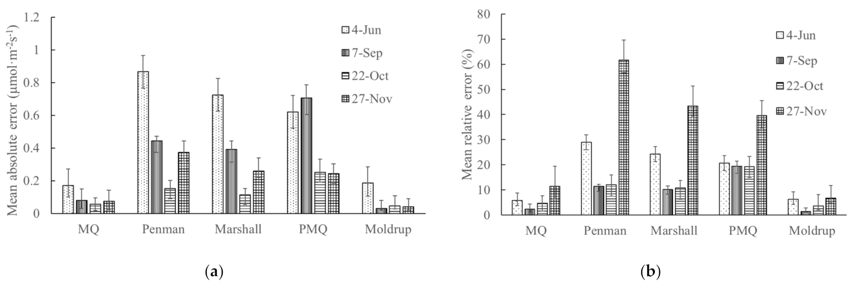
3.5. Measurement of CO₂ Flux in Forest Area

Figure 8 shows the variations of soil CO₂ flux measured by LI-8100 and the gradient method using five diffusion models on days 4 June, 7 September, 22 October and 27 November in 2020. The estimated soil CO₂ fluxes by the gradient method with the Moldrup model are the closest to the measurements of LI-8100. Figure 9 demonstrates the absolute error and relative error of soil CO₂ fluxes measured by the gradient method and LI-8100. Good agreements can be found between the results measured by LI-8100 and the gradient method using the Moldrup model and the MQ model. In the four-day experimental data showed in Figure 8, the mean absolute error of the soil CO₂ flux calculated by the MQ, Penman, Marshall, PMQ and Moldrup models were 0.095, 0.458, 0.372, 0.455 and 0.076 μmol·m⁻² s⁻¹, respectively, and the mean relative errors were 6.05%, 28.51%, 22.14%, 24.73% and 4.51%, respectively. It can be seen that the performances of the Moldrup model and the MQ model in evaluating soil CO₂ flux in the forest area are satisfactory, and the Moldrup model is slightly better than the MQ model, which is consistent with the experimental results in the laboratory.

4. Conclusions

In this study, we analyzed and compared the five commonly used diffusion models (the MQ, Penman, Marshall, PMQ and Moldrup models) for calculating ξ in the gradient method in order to estimate soil CO₂ flux when soil moisture, bulk density and fertility status were changed. The estimates with the five models were compared with the results measured by the alkali absorption method in the laboratory and by LI-8100 in the forest farm. The correlation analysis between the model calculations and the measurements in the laboratory and the error analysis in the forest farm confirmed that the estimating accuracy of the Moldrup model is the highest, followed by the Millington–Quirk model, while those of the Penman, Marshall and Penman–Millington–Quirk models are poor. Moreover, K and P fertilizer had little effect on the soil CO₂ flux, but organic fertilizer (fermented chicken manure) could significantly increase the soil CO₂ flux. In general, soil CO₂ flux estimated by the gradient method is highly sensitive to the diffusion model and insensitive to variable soil properties, and the gradient method can be used as a practical, cost-effective tool to measure soil CO₂ flux only when the appropriate diffusion model is first determined.

References

1. Law, B.E.; Kelliher, F.M.; Baldocchi, D.D.; Anthoni, P.M.; Irvine, J.; Moore, D.; Tuyl, S.V. Spatial and temporal variation in respiration in a young ponderosa pine forest during a summer drought. Agric. For. Meteorol. 2001, 110, 27–43. [Google Scholar] [CrossRef]
2. Rodeghiero, M.; Cescatti, A. Main determinants of forest soil respiration along an elevation/temperature gradient in the Italian Alps. Glob. Chang. Biol. 2005, 11, 1024–1041. [Google Scholar] [CrossRef]
3. Wang, T.L. New ideas cultivate high-value permanent forests. Land Green 2017, 9, 4–17. [Google Scholar]
4. Huang, F.; Cao, J.H.; Zhu, T.B.; Fan, M.Z.; Ren, M.M. CO2 Transfer characteristics of calcareous humid subtropical forest soils and associated contributions to carbon source and sink in Guilin, Southwest China. Forests 2020, 11, 219. [Google Scholar] [CrossRef] [Green Version]
5. Zhang, K.D.; Gong, Y.; Francisco, J.E.; Bracho, R.; Zhang, X.Z.; Zhao, M. Measuring multi-scale urban forest carbon flux dynamics using an integrated eddy covariance technique. Sustainability 2019, 11, 4335. [Google Scholar] [CrossRef] [Green Version]
6. Campioli, M.; Malhi, Y.; Vicca, S.; Luyssaert, S.; Papale, D.; Peñuelas, J.; Reichstein, M.; Migliavacca, M.; Arain, M.A.; Janssens, I.A. Evaluating the convergence between eddy-covariance and biometric methods for assessing carbon budgets of forests. Nat. Commun. 2016, 7, 13717. [Google Scholar] [CrossRef]
7. Massman, W.J.; Lee, X. Eddy covariance flux corrections and uncertainties in long-term studies of carbon and energy exchanges. Agric. For. Meteorol. 2002, 113, 121–144. [Google Scholar] [CrossRef]
8. Ngao, J.; Epron, D.; Delpierre, N.; Breda, N.; Granier, A.; Longdoz, B. Spatial variability of soil CO2 efflux linked to soil parameters and ecosystem characteristics in a temperate beech forest. Agric. For. Meteorol. 2012, 154, 136–146. [Google Scholar] [CrossRef]
9. Pumpanen, J.; Kolari, P.; Ilvesniemi, H.; Minkkinen, K.; Vesala, T.; Niinistö, S.; Lohila, A.; Larmola, T.; Morero, M.; Pihlatie, M.; et al. Comparison of different chamber techniques for measuring soil CO2 efflux. Agric. For. Meteorol. 2004, 123, 159–176. [Google Scholar] [CrossRef]
10. Acosta, M.; Darenova, E.; Krupková, L.; Pavelka, M. Seasonal and inter-annual variability of soil CO2 efflux in a Norway spruce forest over an eight-year study. Agric. For. Meteorol. 2018, 256-257, 93–103. [Google Scholar] [CrossRef]
11. Maier, M.; Schack-Kirchner, H. Using the gradient method to determine soil gas flux: A review. Agric. For. Meteorol. 2014, 192–193, 78–95. [Google Scholar] [CrossRef]
12. Myklebust, M.; Hipps, L.; Ryel, R. Comparison of eddy covariance, chamber, and gradient methods of measuring soil CO2 efflux in an annual semi-arid grass, Bromus tectorum. Agric. For. Meteorol. 2008, 148, 1894–1907. [Google Scholar] [CrossRef]
13. Wolf, B.; Chen, W.; Brüggemann, N.; Zheng, X.; Pumpanen, J.; Butterbach-Bahl, K. Applicability of the soil gradient method for estimating soil–atmosphere CO2, CH4, and N2O fluxes for steppe soils in Inner Mongolia. J. Plant Nutr. Soil Sci. 2011, 174, 359–372. [Google Scholar] [CrossRef]
14. Han, W.; Gong, Y.S.; Ren, T.S.; Horton, R. Accounting for time-variable soil porosity improves the accuracy of the gradient method for estimating soil carbon dioxide production. Soil Sci. Soc. Am. J. 2014, 78, 1426–1433. [Google Scholar] [CrossRef]
15. Wang, C.; Huang, Q.B.; Yang, Z.J. Analysis of vertical profiles of soil CO2 efflux in Chinese fir plantation. Acta Ecol. Sin. 2011, 31, 5711–5719. [Google Scholar]
16. Pu, X.T.; Lin, W.S.; Yang, Y.S. Vertical profile of soil CO2 flux in a young Chinese fir plantation in response to soil warming. Acta Sci. Circumstantiae 2017, 37, 288–297. [Google Scholar]
17. Masakazu, O.; Hiromi, Y. Forest floor CO2 flux estimated from soil CO2 and radon concentrations. Atmos. Environ. 2010, 44, 4529–4535. [Google Scholar]
18. Davidson, E.A.; Trumbore, S.E. Gas diffusivity and production of CO2 in deep soils of the eastern amazon. Tellus B 1995, 47, 550–565. [Google Scholar] [CrossRef] [Green Version]
19. Tang, J.W.; Baldocchi, D.D.; Ye, Q.; Xu, L. Assessing soil CO2 efflux using continuous measurements of CO2 profiles in soils with small solid-state sensors. Agric. For. Meteorol. 2003, 118, 207–220. [Google Scholar] [CrossRef]
20. Riveros-Iregui, D.A.; McGlynn, B.L.; Epstein, H.E.; Welsch, D.L. Interpretation and evaluation of combined measurement techniques for soil CO2 efflux: Discrete surface chambers and continuous soil CO2 concentration probes. J. Geophys. Res. Biogeosci. 2008, 113, G4. [Google Scholar] [CrossRef] [Green Version]
21. Sullivan, B.W.; Dore, S.; Kolb, T.E.; Hart, S.C.; Montes-Helu, M.C. Evaluation of methods for estimating soil carbon dioxide efflux across a gradient of forest disturbance. Glob. Chang. Biol. 2010, 16, 2449–2460. [Google Scholar] [CrossRef]
22. Vargas, R.; Allen, M.F. Environmental controls and the influence of vegetation type, fine roots and rhizomorphs on diel and seasonal variation in soil respiration. New Phytol. 2008, 179, 460–471. [Google Scholar] [CrossRef] [PubMed] [Green Version]
23. Pingintha, N.; Leclerc, M.Y.; Beasley, J.P.; Zhang, G.; Senthong, C. Assessment of the soil CO2 gradient method for soil CO2 efflux measurements: Comparison of six models in the calculation of the relative gas diffusion coefficient. Chem. Phys. Meteorol. 2010, 62, 47–58. [Google Scholar] [CrossRef]
24. Enrique, P.; Sánchez, C.; Russell, L.S.; Joost, H.; Greg, A.B. Improving the accuracy of the gradient method for determining soil carbon dioxide efflux. J. Geophys. Res. Biogeosci. 2017, 122, 50–64. [Google Scholar]
25. Wang, Y.W.; Luo, W.J.; Zeng, G.N.; Yang, H.L.; Wang, M.F.; Lyu, Y.; Cheng, A.Y.; Zhang, L.; Cai, X.L.; Chen, J.; et al. CO2 flux of soil respiration in natural recovering karst abandoned farmland in Southwest China. Acta Geochim. 2020, 39, 527–538. [Google Scholar] [CrossRef]
26. Jones, H.G. A quantitative approach to environmental plant physiology. In Plants and Microclimate; Cambridge University Press: New York, NY, USA, 1992; p. 428. [Google Scholar]
27. Millington, R.J.; Quirk, J.P. Permeability of porous solids. Trans Actions Faraday Soc. 1961, 57, 1200–1207. [Google Scholar] [CrossRef]
28. Penman, H.L. Gas and vapour movements in the soil: I. The diffusion of vapours through porous solids. J. Agric. Sci. 1940, 30, 437–462. [Google Scholar] [CrossRef]
29. Marshall, T.J. Gas diffusion in porous media. Science 1959, 130, 100–102. [Google Scholar]
30. Moldrup, P.; Olesen, T.; Rolston, D.E. Modeling diffusion and reaction in soils: VII. Predicting gas and ion diffusivity in undisturbed and sieved soils. Soil Sci. 1997, 162, 632–640. [Google Scholar] [CrossRef]
31. Moldrup, P.; Olesen, T.; Gamst, J. Predicting the gas diffusion coefficient in repacked soil: Water-induced linear reduction model. Soil Sci. Soc. Am. J. 2000, 64, 1588–1594. [Google Scholar] [CrossRef]
32. Zhao, Y.D.; Wang, Y.M. Study on the measurement of soil water content based on the principle of standing-wave ratio. Trans. Chin. Soc. Agric. Mach. 2002, 4, 109–111. [Google Scholar]
33. Zhou, Z.; Xia, W.B.; Wang, F.; Li, X.W.; Chen, Q.; Yang, X.L.; Chen, X.Y. Soil CO2 flux change and its effect factors from 4 different land use types in Huainan city. Urban Environ. Urban Ecol. 2016, 29, 22–25. [Google Scholar]
34. Sun, J.; Yu, X.X.; Li, H.Z.; Chang, Y.; Wang, H.N.; Tu, Z.H.; Liang, H.R. Simulated erosion using soils from vegetated slopes in the Jiufeng Mountains, China. Catena 2016, 136, 128–134. [Google Scholar] [CrossRef]
35. Ayers, P.D.; Perumpral, J.V. Moisture and density effect on cone index. Trans. ASAE 1982, 25, 1169–1172. [Google Scholar] [CrossRef]
36. Yan, X.F.; Zhao, Y.J.; Cheng, Q.; Zheng, X.L.; Zhao, Y.D. Determining forest duff water content using a low-cost standing wave ratio sensor. Sensors 2018, 18, 647. [Google Scholar] [CrossRef] [Green Version]
37. Zhu, M.Z.; Xue, W.L.; Xu, H.; Gao, Y.; Zhang, Z. Diurnal and seasonal variations in soil respiration of four plantation forests in an urban park. Forests 2019, 10, 513. [Google Scholar] [CrossRef] [Green Version]
38. Strack, M.; Waddington, J.M.; Tuittila, E.S. Effect of water table drawdown on northern peatland methane dynamics: Implications for climate change. Glob. Biogeochem. Cycles 2004, 18, 1–7. [Google Scholar] [CrossRef] [Green Version]
39. Munir, T.M.; Perkins, M.; Kaing, E.; Strack, M. Carbon dioxide flux and net primary production of a boreal treed bog: Responses to warming and water-table-lowering simulations of climate change. Biogeosciences 2015, 12, 1091–1111. [Google Scholar] [CrossRef] [Green Version]
40. Munir, T.M.; Khadka, B.; Xu, B.; Strack, M. Mineral nitrogen and phosphorus pools affected by water table lowering and warming in a boreal forested peatland. Ecohydrology 2017, 10, e1893. [Google Scholar] [CrossRef]
41. Chimner, R.A.; Pypker, T.G.; Hribljan, J.A.; Moore, P.A.; Waddington, J.M. Multi-decadal changes in water table levels alter peatland carbon cycling. Ecosystems 2017, 20, 1042–1057. [Google Scholar] [CrossRef]
42. Tan, J.R.; Zha, T.G.; Zhang, Z.Q. Effects of soil temperature and moisture on soil respiration in a poplar plantation in Daxing district, Beijing. Ecol. Environ. Sci. 2009, 18, 2308–2315. [Google Scholar]
43. Epron, D.; Farque, L.; Lucot, E. Soil CO2 efflux in a beech forest: Dependence on soil temperature and soil water content. Ann. For. Sci. 1999, 56, 221–226. [Google Scholar] [CrossRef] [Green Version]
44. Moldrup, P.; Olesen, T.; Komatsu, T.; SchjØnning, P.; Rolston, D.E. Tortuosity, diffusivity, and permeability in the soil liquid and gaseous phases. Soil Sci. Soc. Am. J. 2001, 65, 613–623. [Google Scholar] [CrossRef]
45. Moldrup, P.; Olesen, T.; Komatsu, T.; Yoshikawa, S.; SchjØnning, P.; Rolston, D.E. Modeling diffusion and reaction in soils: X. A unifying model for solute and gas diffusivity in unsaturated soil. Soil Sci. 2003, 168, 321–337. [Google Scholar] [CrossRef]
Figure 1. Schematic of the system for measuring soil CO2 concentration, moisture and temperature profiles.
Sustainability 13 10874 g001
Figure 2. The encased CO2 probe (a) and the self-developed moisture sensor (b).
Sustainability 13 10874 g002
Figure 3. Photograph (a) and diagram (b) of the soil vertical profile CO2 concentration monitoring experiment.
Sustainability 13 10874 g003
Figure 4. Simultaneous measurement of soil CO2 flux by the chamber method and the gradient method in the forest area.
Sustainability 13 10874 g004
Figure 5. Absolute error (a) and relative error (b) of determination of CO2 flux by concentration gradient method and alkali absorption method at different water contents.
Sustainability 13 10874 g005
Figure 6. Absolute error (a) and relative error (b) of determination of CO2 flux by concentration gradient method and alkali absorption method at different soil bulk densities.
Sustainability 13 10874 g006
Figure 7. Absolute error (a) and relative error (b) of determination of CO2 flux by concentration gradient method and alkali absorption method at different fertility status.
Sustainability 13 10874 g007
Figure 8. Soil CO2 flux measured by LI-8100 and the gradient method using five diffusion models on days 4 June (a), 7 September (b), 22 October (c) and 27 November (d) in 2020.
Sustainability 13 10874 g008aSustainability 13 10874 g008b
Figure 9. Absolute error (a) and relative error (b) of soil CO2 fluxes measured by LI-8100 and the gradient method with five diffusion models.
Sustainability 13 10874 g009