Integrated Water-Power System Resilience Analysis in a Southeastern Idaho Irrigation District: Minidoka Case Study

Abstract

This study investigates the joint water–power system resilience of an irrigation district in southeastern Idaho. Irrigation districts face difficulties in the delivery of water to farmers under drought conditions, during equipment failures, or unplanned infrastructure disruptions. The resilience of interconnected water and power systems can be better analyzed and understood through an integrated approach, using a model that connects the dependencies between the two halves of the system. Using a multi-agent system model capturing both water and power system components, as well as their linkages, we capture the interdependencies of these systems and highlight opportunities for improvement when faced with disruptions. Through simulation scenarios, we examine the system resilience using system performance, quantified as the percentage of met demand of the power and water system, when subjected to drought water year, an unforeseen water demand increase, power outage and dam failure. Scenario results indicate that the effects of low flow years are mostly felt in the power system; unexpected increases in water demand marginally impact irrigation system performance; dams and pumps present vulnerabilities of the system, causing substantial unmet demand during disruptions. Noting the interdependencies between the water–power system halves while leveraging an integrated simulation allows for an insightful analysis of the system impacts during disruptions.

1. Introduction

Power and water infrastructure systems rely on their interdependence to ensure their service requirements, i.e., to meet power and water demand requirements, respectively. Generating units available in power systems should be dispatched appropriately to ensure a reliable delivery, whenever, wherever and of whatever quantity to consumers, which can be of commercial, industrial, and residential types. The same phenomenon is observed in water systems, with water sources designed to supply demands, which can be of non-irrigation (residential, commercial, and industrial, etc.) and irrigation types. Power and water sources require each other to function. For instance, water treatment systems require electricity for pumping, treatment and distribution [1,2] and thermal-based generation (e.g., nuclear, coal, natural gas) require some water for cooling [3,4]. While the nexus between power and water generation presents many opportunities for efficiencies, cost savings, and a more sustainable environment [5,6,7], it also presents challenges. Water scarcity, demand variability, and uncertainty are becoming more prominent, leading to vulnerabilities in the U.S. energy system [8]. It is therefore critical to employ a more integrated approach to address these challenges, holding promise of support for an improved resource use efficiency.

Our study mainly focuses on irrigation systems, which were historically designed to capture and store water at higher elevations and to deliver it to lower elevations primarily using gravity (Figure 1). The reservoir represents water storage, from where water is withdrawn at the needed rate. This rate is determined by the positioning of head gates. Diversion structures separate all or part of the flow and supply the canals. Additional headgates control the flow of water into laterals, which divert water from canals to irrigation sites. Weirs are used to control the flow of water from outlets of laterals or ponds, raising the water level as needed for the required amount to be carried to irrigating fields, via ditches.

Modern irrigation infrastructures are designed to improve efficiency by reducing seepage and evaporation losses from open channels, improving conveyance, enabling the use of sprinklers and drip irrigation relying on pressurized systems, and to optimize energy and water usage through the use of pump scheduling, sensors and communication networks [9,10,11]. Structural infrastructure improvements can increase efficiency and resilience by reducing water seepage and evapotranspiration, which in turn increases the supply of water by decreasing conveyance losses. Similarly, installing or utilizing existing local energy resources, like small hydroelectric, solar, wind and/or battery storage provides the ability to serve irrigation system power needs, thereby enhancing reliability and resilience against events that disrupt electricity transmission or distribution. Gravity fed storage of water is another source that allows for irrigation to continue for some period of time during disruptions to power or water infrastructure.

Just as irrigation systems represent a significant portion of water withdrawals in the US, they also account for a significant portion of electrical demand. Particularly in the Western US, agricultural pumping accounts for approximately 2.6% of electricity use [12]. An irrigation system addresses irrigation needs in a timely manner while minimizing losses and damage to crop quality. In this sense, it is critical that the amount of water needed is at the right amount, the right place and the right time. Such disposition requires good planning, ensuring all interdependencies are taken into account, not only under normal conditions, but also and more importantly during disruptions. Water and power in irrigation systems are typically linked through components such as pumps, in-conduit hydropower generation, sprinklers, and controls for gates and valves. The precise linkages vary considerably by context. For example, systems that are predominantly gravity-fed and that were designed a century ago may have less reliance on power for their operation. In contrast, modernized systems that use digital controls and include local power generation may have greater water–power interdependence. This can be a benefit in providing greater optimization, more potential revenue streams, and lower operational and maintenance costs.

Energy, in the form of electricity, is input to the water system to control head, water flow rate, and direction in canals to carry water. The injected power enables the activation of various powered physical control devices such as head gates, valves, pumps and other diversion structures, responsible for water flow and distribution. This amount of energy also needs to be planned for, to ensure power grid system balance. As planning is done in the water system, operators assess the power source usage and determine the expected power generation to meet demands. While dams constitute an energy storage and power source via hydropower, it is also a water source, serving irrigation purposes. As such, it represents another critical linkage point between those two systems, as electricity generation depends on the proportion of water assigned to it, which is intricately linked to the proportion of water assigned to irrigation.

Despite these linkages, water and power systems are often viewed as serving either water-based objectives or power-based objectives during the design and operation phases. The importance of the dependencies is more acutely perceived when challenges emerge. The existence and availability of tanks or reservoirs for water storage provides a mechanism to supply water demands during periods of scarcity. Water can be stored by pumping when power demand is low and electricity is cheaper, and can then be released to supply water demands during peak hours, reducing the cost of electricity consumption. At the same time, water stored can supply water demands, in case of limitations in water availability or operating issues at treatment facilities. The water stored can also be used for small-scale, pumped storage hydropower generation. The power generated from these sources can be used for supplying (1) the pumping power requirements in the irrigation district, minimizing the impact of the disruption and also maintaining the operation of the water irrigation system, and (2) the power demand, especially in the case of disruption.

From this general perspective, the interdependence of these infrastructures not only allows its normal operation, but also leverages the capability of both systems to maintain its operational conditions, even in the case of contingencies. This represents opportunities for enhancements in the robustness of both power and water systems, and ultimately calls for an integrated approach for resilience. To that effect, the U.S. government’s National Infrastructure Protection Plan-2013 stated that “the extent to which infrastructure is interconnected shapes the environment for critical infrastructure security and resilience” [13].

This is where our contribution lies: assessing water and power system resilience of an irrigation district in a rural area, through the lens of system interdependencies. The central research question can be formulated as: How can interdependencies be leveraged to analyze the impacts on the water system due to events originating in the power system, or the inverse? Given the linkages between these systems, the integrated system’s performance cannot be investigated by analyzing the performance of its subsystems taken in isolation from one another [14]. Integration of multiple sub-systems requires compatibility between them, and it is critical to identify the characteristics of, and the dependencies between, each, using appropriate modeling tools. We are using a multi-agent-based simulation model, which involves an object-oriented approach to simulate water and power system operations. The modelling platform used captures the interdependency of power and water systems for an integrated analysis to better inform resilience planning. A number of modeling efforts have been undertaken to address energy-water nexus challenges. Payet-Burin et al. [15], Vinca et al. [16] and Saif and Almansoori [17] present a modeling approach to optimize energy, water and land decisions, subject to future socioeconomic and climatic change. The GIS-based model by Almulla et al. [18] estimates water and electricity requirements for groundwater irrigation in various locations to suggest more effective supply options and least-costly configurations. These models are built for long-term planning and/or capacity expansion decisions to meet some sustainability targets, and are thus not appropriate for our purpose. Other models in the literature represent either system in a coarse manner [19,20,21,22], mostly geared toward the performance of one system, or the other, with no holistic view of the whole system. The model we present in this paper offers a more functional oriented representation of both the power system and the water system, with detailed operation and co-management features with contingency components represented. The modeling approach presented remains at a level of detail adapted to the practical simulation of management of large and complex systems, representing energy/water management strategic functions like generation, distribution, or regulation, with components responsible for the operations of these functions.

In the next section, we review the notion of resilience and define our metrics of interest. Section 2 presents the model used for analysis. Section 3 defines the case study and specifies the system boundaries, results and implications. Discussion and conclusion ensue in Section 4.

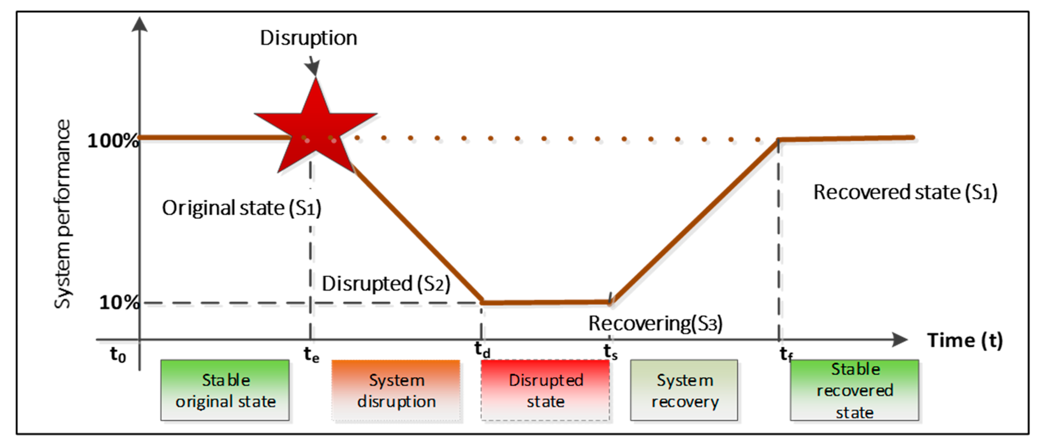
Defining Resilience

In this article, a resilience study is conducted on an irrigation district system located in Southeastern Idaho. A resilient system is one that maintains state awareness and an accepted level of operational normalcy in response to disturbances [23,24,25]. Figure 2 gives a snapshot of the system performance before, during and after disruption. In each of these periods, we observe a different state, as state transitions determine the level of performance of the system. Disruptions lead to an impairment and potential loss of service, in water or/and power to end-users. The mechanism, timing, and duration of the disruption are critical factors in the outcome of these measures. If the precipitating causes of the disruptive event are short-lived, and the failure mechanism is easily overcome, then the disruption will be small, and the perceived resilience of the system will be large, as it will quickly recover from a partially perturbed state. For the power system, system performance metrics used in previous studies include power supply reduction, households/farms/area without power [26] and ratio of power supply to demand [27]. Similarly, for the water system, water supply reduction, households/farms/area without water and ratio of water supply to demand have been used. In our study, resilience would be estimated through the analysis of system performance, quantified as the ratio of actual water/power available for release to the water/power demand during a given period of time.

Figure 3a,b illustrate the main idea of this paper, which is the impact assessment of disruption on interconnected power and water systems. Resilience assessment of power and energy systems through their interdependence is beneficial, as it can help (1) understand both systems ability to absorb a disruption and the effect it has on their performance, and (2) identify critical system components and required infrastructure and modernization needed to improve system performance.

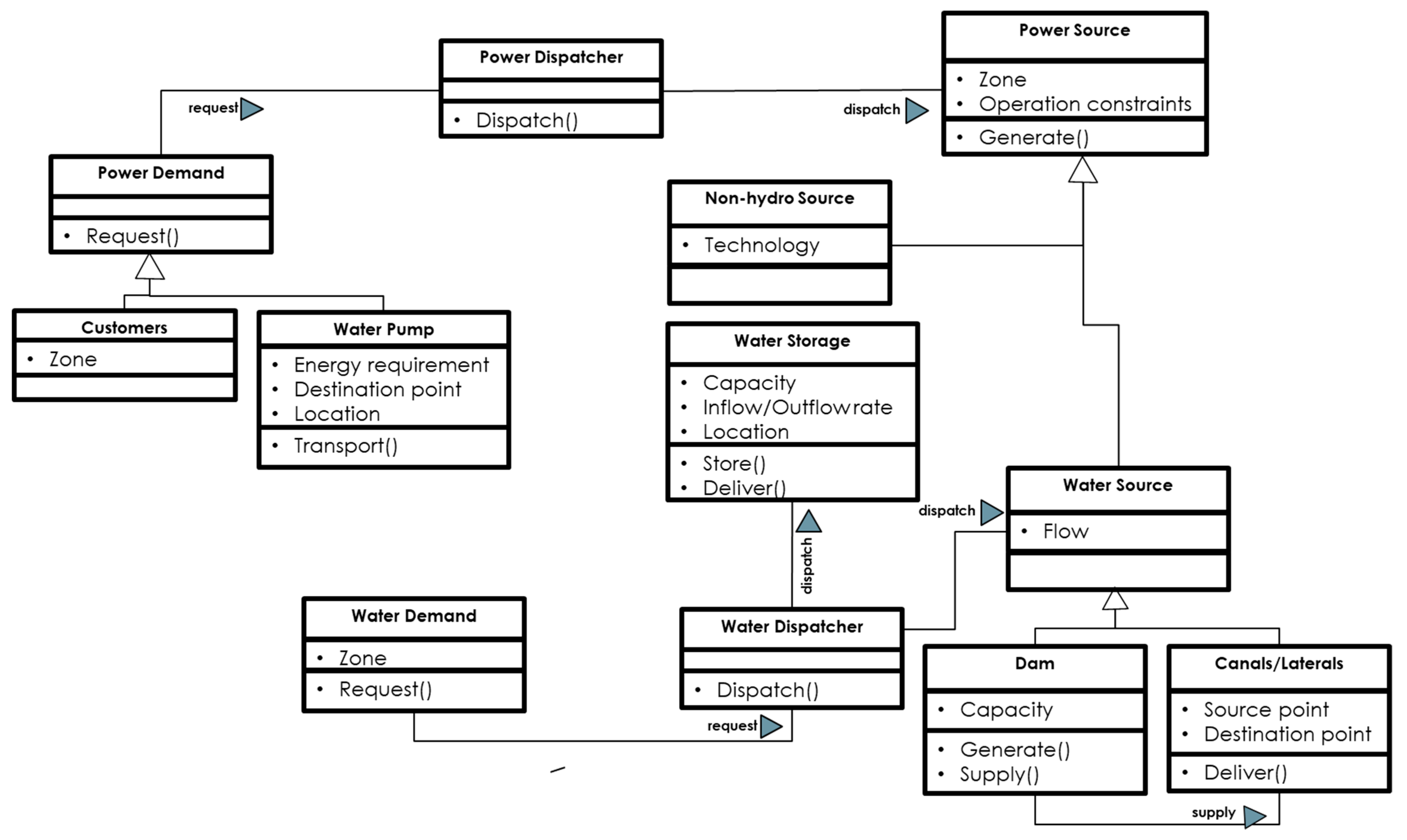
2. Modeling Approach

We present a bottom-up discrete-event dynamic system model that simulates the behavior of an integrated water–power system, considering the combined effects of water system activities on power systems, and vice versa, and their interdependent nature. The integrated power–water system is conceptualized as a rule-based water/power resource management system. The water system is composed of components for the collection, transportation, distribution and use of water. As such, the model represents all the components performing these activities, including water tanks/reservoirs, water canals, water pumps, as well as water demands. The same goes for the power grid system, which is composed of components for the generation, transmission, distribution and use of electricity. The model represents generation sources, distribution components, as well as power demands. All these components are represented as agents, built as event-based dynamical systems, interacting with each other [28].

Figure 4 shows a simplified Unified Modeling Language (UML) class diagram conceptual model of a water–power system. A class diagram describes the structure of a system by showing the system’s classes, their attributes, operations, and the relationships between objects. Agents are modeled as objects, which are instances of class. The upper section contains the name of the class. The middle section contains the attributes of the class, describing the characteristics of specific objects. For example, water pump agents differ from each other by location, energy requirement and destination point (where the pump takes the water to). The bottom section contains operations/functions, that is, what agents can do.

Figure 4 displays the main agents represented in the model, as well as their interactions with each other. The overall power demand is composed of customers and water pumps and are represented by power demand agents, the aim of which is to request electricity. Water pump agents, representing water pumps, need power to operate; that is, to transport water from one location to another. Customer agents represent the population in need of power for activities. Power source agents, representing all power sources, are characterized by location and operational constraints, and they generate electricity. The power dispatcher agent, representing the grid operator, receives demand requests from all power demand agents and aggregate them. The agent can then dispatch power sources (including hydro and non-hydro sources), making decisions about how much each of these sources should produce, to meet those demands. Water sources are represented by reservoir dam and canals/reservoirs agents, which are used for power generation and irrigation needs. Canal agents deliver water at their destination point, while dam agents supply water (1) to canals for irrigation needs and (2) for power generation. Water source agents thus interact with both power source agents (representing hydro power) and water dispatcher agents for dispatch, to meet demands. Water demand agents, just like customer agents, represent the population in need of water for activities. The water dispatcher agents perform the same action as their counterparts in the power system, by aggregating all water demand and selecting water sources to meet them. We assume no water right issue in this study. The water storage agent, representing water tanks, store water in case of surplus and deliver water when requested by the water dispatcher agent. Water is distributed to all areas if energy requirements of pumps in those areas are met. Pump energy needs are thus part of the power demand. Linkages relevant to irrigation systems are water pumps and water reservoirs, as they serve both irrigation and power generation needs.

Figure 5 shows this simulation flow process. Water and power demand are aggregated by location and are compared with supply. If there is enough supply, the excess is stored in water/energy storage if existing. If not, quantity in storages, if available, is called upon. The system performance (ratio demand to demand met) is then computed. The cycle repeats until the simulation ends. Let us also point out that demand in either system captures the needs of the other. For example, demand in water includes irrigation needs in the water system and also power generation needs in the power system.

This problem characterization is in alignment with grid balancing problems, considering the presence of components responsible for resource scheduling and load balancing across the grid [29], as well as water management systems, which are meant to distribute water resources [30] at the strategic level. The agents considered, as well as their constructed behavior, mimic the real-life operations of the water and power systems. The model’s structure, logic, and causal relationships are, we argue, reasonable for the intended purpose of the model.

3. Case Study Background and Results

3.1. Study Area

The case study is an irrigation district project in the Southeastern region of Idaho, including a dam, Lake Walcott, the North Side Canal and the South Side Canal, the associated laterals, and pumping infrastructure. The purpose of the project is to supply water to the land, to build a reliable source of power, and provide opportunities to develop farmland in the area. The dam supplies irrigation water to the Snake River valley in southern Idaho. Cattle, dairy, potatoes, beets, beans, grains, and irrigated pasture are important agricultural uses for the water supplied to the district. In addition to irrigation water, the project supplies hydroelectric power to the region, covering much of the irrigation pumping requirements in the district and beyond. Surplus power beyond the Bureau of Reclamation (BoR) needs is marketed in the Federal Southern Idaho Power System, overseen by the Bonneville Power Administration [31].

The main dam is a 26.2-m-tall earth fill diversion, storage, and power structure. It retains Lake Walcott, the associated reservoir, with a maximum capacity of just over 259 million cubic meters with over 117.2 million cubic meters as active storage. Water is diverted on either side of the dam into canals, the North Side Canal, and the South Side Canal. For the purposes of this study, the South Side Canal is only considered as an additional outlet from Lake Walcott, and so the irrigation district area fed by this canal was not directly considered for the model. The North Side Canal is the main feeder canal for the dam, providing most of the water to farmers. The North Side Canal is gravity-fed and serves 29,150 hectares of land north of the Snake River, near Rupert, Idaho. The dam produces approximately 28 MW of hydroelectric baseload power for the grid. Figure 6 displays the district with canals, laterals and pumping stations (owned by the district).

The main North Side Canal is approximately 13 km long, extending North and East from Lake Walcott before splitting into 4 major branches. These mostly gravity-fed branches extend across the irrigation district and connect to an extensive network of laterals to carry the water to farmers. Approximately 1200 hectares of farmland are located on localized high-points and are therefore watered by electric pumps. Electric pumps on the North Side of the Snake River utilize approximately 970 kW of power and are serviced by several electric utilities including United Electric co-op, East End Electric, Riverside Electric, and the city of Heyburn. Privately-owned electric pumps are used by most farmers to convey water from their adjacent lateral to their irrigation infrastructure and fields.

3.2. Model Input and Validation

The inputs that drive the model are the water and power demands, water and power demand forecast, weather temperature, wind speeds, water storage/reservoir capacity, power generation sources and water pump-related data (energy requirement and location). See

Table 1. Model input and description.

Data Input	Definition
Water and power demand database	Data about the water and power demand per geographical zone and season. Demand data are determined as explained below.
Water and power source database	Data about the water and power sources per geographical zone and type. Data include factors specific to sources (water flow, dam heads, power mix, etc.) [31,33]
Water pump database	Data about pumps energy requirement and location. (see Table S1 with supplemental document “MID_Pumpstations—clean.xlsx”)
Solar database	Data about solar irradiance and temperature [34]
Wind database	Data about wind speed, locations, and wind turbines [34]

.

Given the difficulty in finding demand data, we use proxies. The municipal water demand is estimated based on the population in the region and demand per capita. According to Stene [35], the population rose from a few thousand people in 1915 to more than 200,000 by the 1980s. We estimate the population in 2019 using the percent growth in the state of Idaho, from 1980 to 2019, which is about 85% [36,37], giving about 370,000 people in the district. The demand per capita is estimated to be 882 L per person on a daily basis [38]. Changes in demand is assimilated to changes in water flow, with streamflow data gathered from the 2019 Minidoka Irrigation District watermaster report [33]. Power demand in the district is estimated based on the overall power demand overseen by the Bonneville Power Administration (BPA), which serves about 12 M people [31]. We assume the district demand to be about 3% that of BPA, considering the ratio between populations. Power and water demand are aggregated, based on the overall demand in the district. The input function for water and power demand is:

$$Dm{d}_t={{\displaystyle \sum }}_{i}dm{d}_i\left(t\right)$$

(1)

where Dmd_t is the aggregated demand at time t, and dmd is the localized demand, with i representing different locations. The wind speed and temperature input used are data recorded at the Minidoka, Idaho weather station [39] for our region of interest. Power generated by other sources, including nuclear and fossil/biomass, is deduced from the energy mix of BPA [31].

Only pumping stations owned by the district are considered in the model. Farmers pumps are not accounted for in this study. Data on district owned pumps were gathered from the irrigation district maps and data repository (See Table S1). The function of these pumps is to carry water through canals up to the farms. We assume the presence of farms in the vicinity of pumping stations (see location of pumps in Figure 6).

For validation, we use historical data. Using the 2007 monthly streamflow (Figure 7a), we simulated the power generation from the dam, and compared it with the actual power generation (Figure 7b).

In Figure 8 we use the Box and Whiskers plots as a validation visual technique to inspect model output and to observe differences between them. The boxes (the interquartile range represented by rectangles) overlap with one another and spread past both medians (red line in the boxes), which indicate that there does not seem to be a statistically significant difference between those 2 outputs. This can also be seen in the mean values (represented here by green triangles), which are not too far from each other. Finally, both outputs display a similar data distribution, positively skewed. Both medians are closer to the lower whisker, below the mean values, with lower whiskers shorter than higher ones in both cases. This comparison, operational validation [42], is conducted to determine whether the model’s output behavior has sufficient accuracy for the model’s intended purpose over its intended applicability. Based on the observations noted above, we can deem the model valid.

3.3. Experiments

Given that the model successfully replicated the aggregate power production by plant in 2007, we incorporated the relevant 2019 data for this part of the region. Supply and demand data used ran from April to October 2019; agricultural water demand drops to 0 during the remaining months as there is no cultivation activity during that time. The system vulnerability was analyzed by comparing demand versus supply to assess scarcity (scarcity occurs when demand exceeds supply), in both water and power. A unique aspect of this study is that it focuses on rural area community, relying on community-managed sources and systems. Given the very high vulnerability of these systems, there is an urgency to find ways to provide improved systems and to support community management [43]. Through simulation scenarios, we examine the system resilience, via system performance, measured as explained in Section 2, when subjected to drought year, unforeseen water demand increase, power outage and dam failure.

The scenarios of interest were generated through a consequence-based approach. The ultimate consequence of relevance to regional stakeholders is decreased revenue for farmers, likely due to a production shortage. Given the process diagram for farm production, it was ascertained that the main threat likely to cause a production shortage is either a low water supply, or a disruption of conveyance infrastructure, such as a pump disruption in the irrigation district. These mid-stream consequences are catalyzed by events such as a low-flow year, unusually high demand, some form of pump maintenance failure, or a regional power failure (Figure 9).

The events which were analyzed were selected due to either their probability of occurrence, or interest from regional stakeholders. The low-flow year was conservatively characterized by the expected inflows from a 10-year drought [44]. A demand increase could be precipitated by a hot and dry growing season, a regional shift in crop type to sugar beets or other high-water-demand crops, power demand or regional growth [45]. Maintenance failures of pumps are fairly rare, but maintenance is anecdotally reported by the irrigation district to occur semi-annually. If a pump does not receive its required maintenance, failure rates are high, the consequences of which are of interest to regional stakeholders. Supporting power infrastructure failing via a failed transformer is estimated to have a 10% probability every year [46]. While a regional power failure occurs much less frequently, the scenario is of interest to regional stakeholders due to the severe disruption this would pose to their conveyance infrastructure. The subsections below explore the various precipitating events and their range of effects on the ultimate consequence of causing a production shortage.

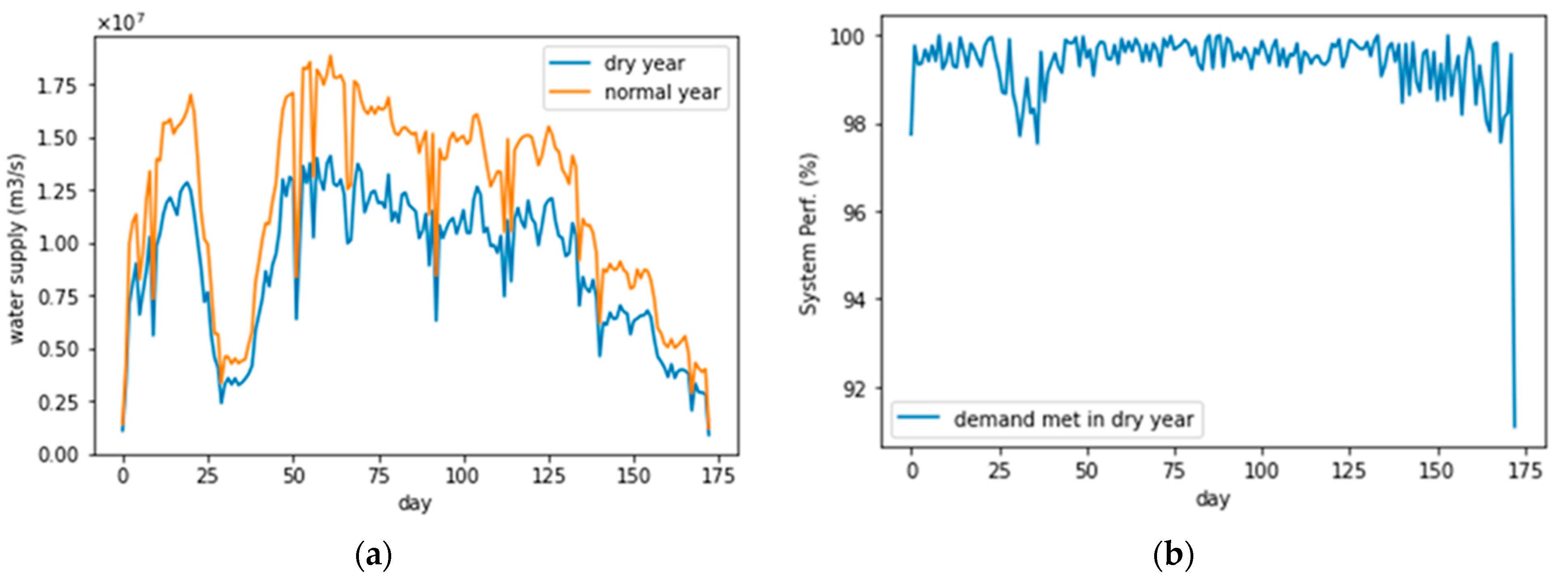
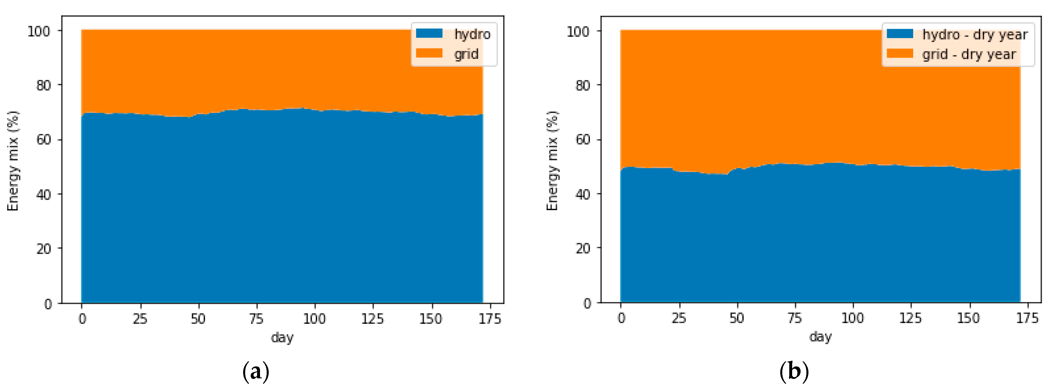
3.3.1. How Does System Function in Normal versus Low Flow Year?

In this first scenario, we investigate the impact of a drought year on both water and power systems. We compare water streamflow to a less-than-normal supply to assess scarcity impacts. This scenario focuses on water supply being between 20% and 30% lower than normal, and the impacts on demand requirements, and implications on power generation.

Figure 10a displays the water supply both during normal and dry years. Normal year sets the expectation for water withdrawals without disruption. Figure 10b displays the proportion of demand met, considering a reduced water supply. A system performance of 1 indicates that all the demand has been met. In our case, we observe between about 1% to 2% for the most part, of the demand goes unmet in a drought year. Such unsatisfactory delivery can push inhabitants/farmers to take coping measures, like investments in storage tanks and retention ponds for instance, requiring out-of-pocket expenses [47]. A study conducted in a city of 300,000 inhabitants in the state of Uttar Pradesh in India revealed significant costs incurred by families, regardless of income levels, to face intermittent water supply disruptions [48]. The impacts of this water stress are also felt in the power system, with a shift in the energy mix in the district, as shown in Figure 11a,b. The energy mix here captures use of energy sources owned by the district (hydro, wind, nuclear, gas, biomass and solar) and does not account for privately owned installations (solar or wind for instance). The amount of power generated by hydro plants is also reduced from about 70% to 50%, placing the burden on other energy supply sources. Such a shift could potentially cause an increase in electricity generation costs, as more production will have to come from more expensive other sources. Other sources in the area include wind, fossil/biomass and nuclear generation [31]. Besides the impacts on energy mix and power from hydro plants, there are also impacts on thermoelectric generation. Reductions in water flow and supply can have substantial impacts on thermal power plant power generation, as cooling systems are the most water-intensive part of the thermoelectric generation process [49].

Low flow years are fairly common in this area [44]. The common occurrence of droughts of this severity in the area, combined with the resulting effects to unmet irrigation system demand and energy mix, indicate that it is important for system owners to take more serious steps toward the resilience of the system.

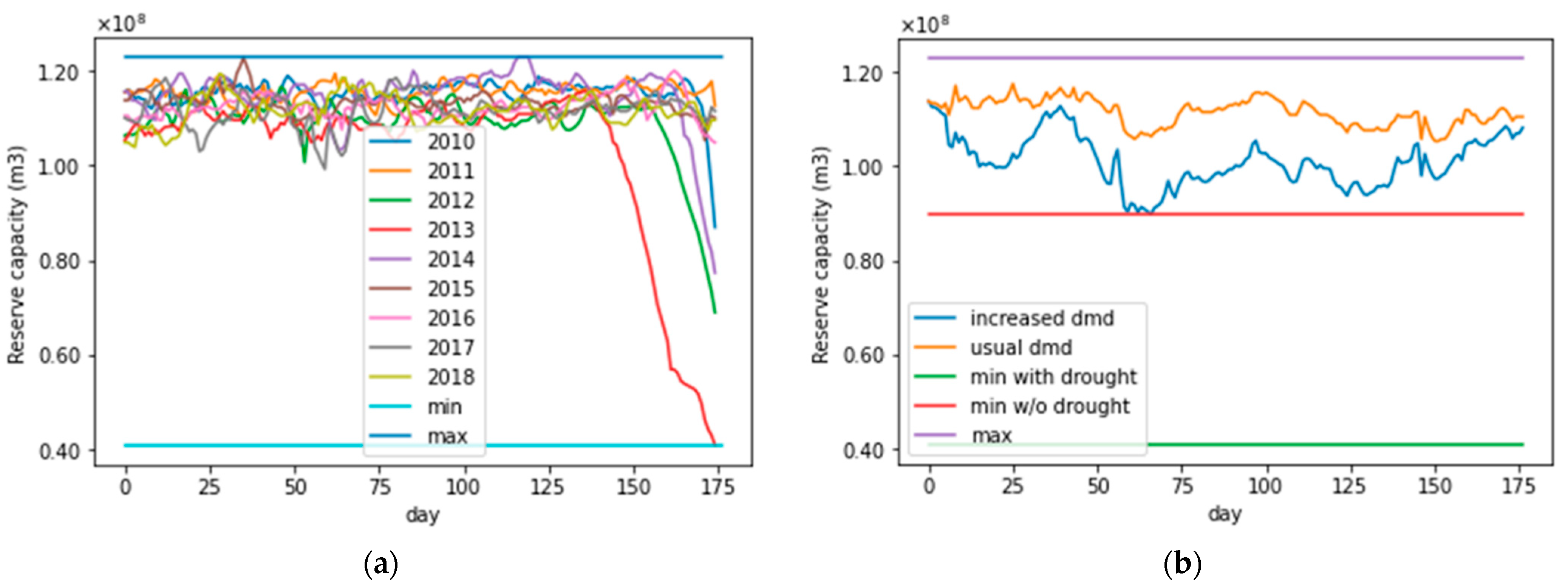
3.3.2. How Does the System Function in Situations of Water Demand Increase?

In the second scenario, we investigate the impact of a 15% water demand increase on the integrated water and power systems. Figure 10b shows the reservoir levels both when in normal use and when demand is increased. The normal use here represents the real reservoir storage level over the same period of time, obtained from the Bureau of Reclamation [50]. In the event of an unforeseen demand rise, the reservoir is used at an additional 10% of its normal use. This indicates a fairly good level of reliability. With a full capacity of 117,399,021 cubic meters [51], an increased demand of 15% pushes the available capacity to about 86% full, compared to a 94% use of its capacity in normal use, over the growing season time period considered.

Figure 12a shows the historical values of reservoir usage from year 2010 until 2018, obtained from the BoR [40]. These data are used as a proxy, to estimate the minimum (lowest level since year 2010) and maximum (highest level since year 2010) operational levels. It can be observed, despite the rise in demand, that the reservoir level remains significantly higher than the lowest level over the past decade, with the lowest point representing 2.2 times that of the minimum level. Although we also notice that compared to other years, reservoir levels in 2012, 2013 and 2014 drop significantly, indicating dry years in the region (see [52]).

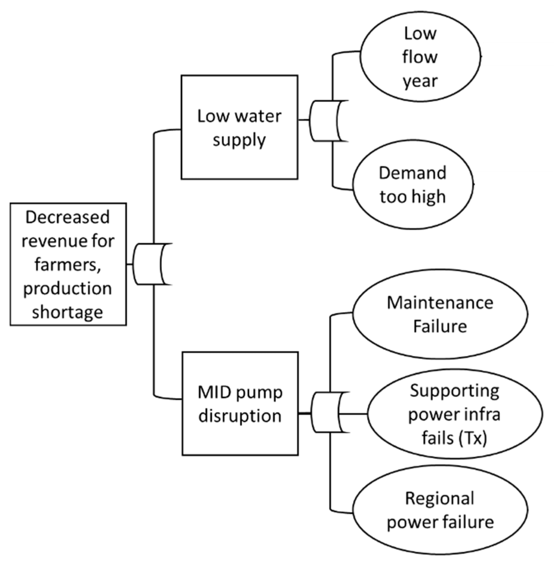
3.3.3. How Does the System Function in the Situation of Pump Failure/Power Outage?

In the third scenario, we investigate the impact of pump failure throughout the system for the whole season. We look to assess the effects of eventual power outage or mechanical failure on the system performance. We consider two pumping stations for this scenario, namely Trantham and Murphy stations. These present spatially different profiles, as one is located far upstream on a canal that supplies other canals, with additional pumps, while the other is located at the end of a canal (see Figure 6). Given the lack of data regarding farm demands across the region, we assume that demand and deficit are spread based on the location of the pumps. The presence of pumps is justified by changes in elevation; that is, if water is required to flow from a low to a high head, pumps are used to artificially increase the head on the side of the incoming flow, so that water continues to flow in the same direction to reach farms. In the presence of a gravity-fed system, where water is naturally flowing from higher heads, they are unnecessary.

Figure 13a,b show the impacts of localized mechanical pump failure or power outage for the entire season, altering the normal flow of water to farmers. The impact is felt more in the case of pumping station Trantham as it carries water to multiple canals downstream. As a result, on average, about 21% of demand goes unmet, while this is only 2% for the Murphy pumping station, over the whole district area. Farms located near canals downstream of the Trantham pumping station will not receive the needed amount of water.

3.3.4. How Does the System Function in a Situation where the Reservoir Is Empty?

In the fourth scenario, we investigate the impact of a dam failure, causing the water in the reservoir to be completely unusable. In this case, water demand goes unmet. We look at the effects on the power system. As part of the water from the reservoir is used for power generation, a failed dam would cause power loss [53]. It is important to note that the energy sources considered are the ones owned by the district. Figure 14 illustrates how much power deficit there will be if only these sources were used to face a dam failure situation. Because this is not an islanded system, it is fair to assume that power from other utilities or neighboring areas may offset the deficit. However, the intention here is to highlight the system vulnerability in our area of interest, as outside systems are out of the scope of this study.

Figure 14 shows the amount of power met in the situation of dam failure, with less than 65% of demand satisfied. This shows how much power generation will be expected from imports. According to BPA [31], about 80% of power generated comes from water over the region serviced. Considering the large proportion of hydro generation, a dam failure would have devastating consequences at the power distribution level, with a shift in the energy mix. In the absence of water, supply would have to exclusively come from other sources, potentially impacting costs. The scheduling and dispatch of generation sources is done in an economic manner; that is, plants with the lowest variable operating costs are generally brought on first, then, as demand rises, plants with higher variable operating costs are sequentially dispatched [54]. With hydro (being the lowest-cost source of electricity globally [55]) not available, other higher cost sources including gas, nuclear, wind, biomass and solar would be used. The higher fuel prices, especially natural gas, would contribute to increasing electricity costs. Another aspect is transmission costs due to imports. With a high proportion of demand going unmet, imports are likely to be needed. Electricity transmission and distribution systems connecting plants with consumers have operation and maintenance costs [56] which would contribute to consumption price increases. Beyond costs implications, there are also operational implications to consider, with the loss of flexibility caused by an absence of hydrogeneration. Hydropower is a flexible resource, which can supply or store electricity to meet real-time energy needs [57]. This makes hydro sources complementary to other forms of generation, as they could, for instance, store excess electricity from coal or nuclear sources. Given the emergence of renewable sources bringing more variability into power generation, hydropower can help stabilize the grid [58,59], keeping power supplies constant. Flexibility in the grid provides the ability of supply sources to respond to the variation and uncertainty in net load [60]. This is therefore critical from a resilience or reliability standpoint. By contributing to a diverse energy mix like the one in the southeastern Idaho region, hydropower therefore protects energy independence, strengthens the reliability of the system, and reduces the system reliance on imported electricity, especially from fossil fuels.

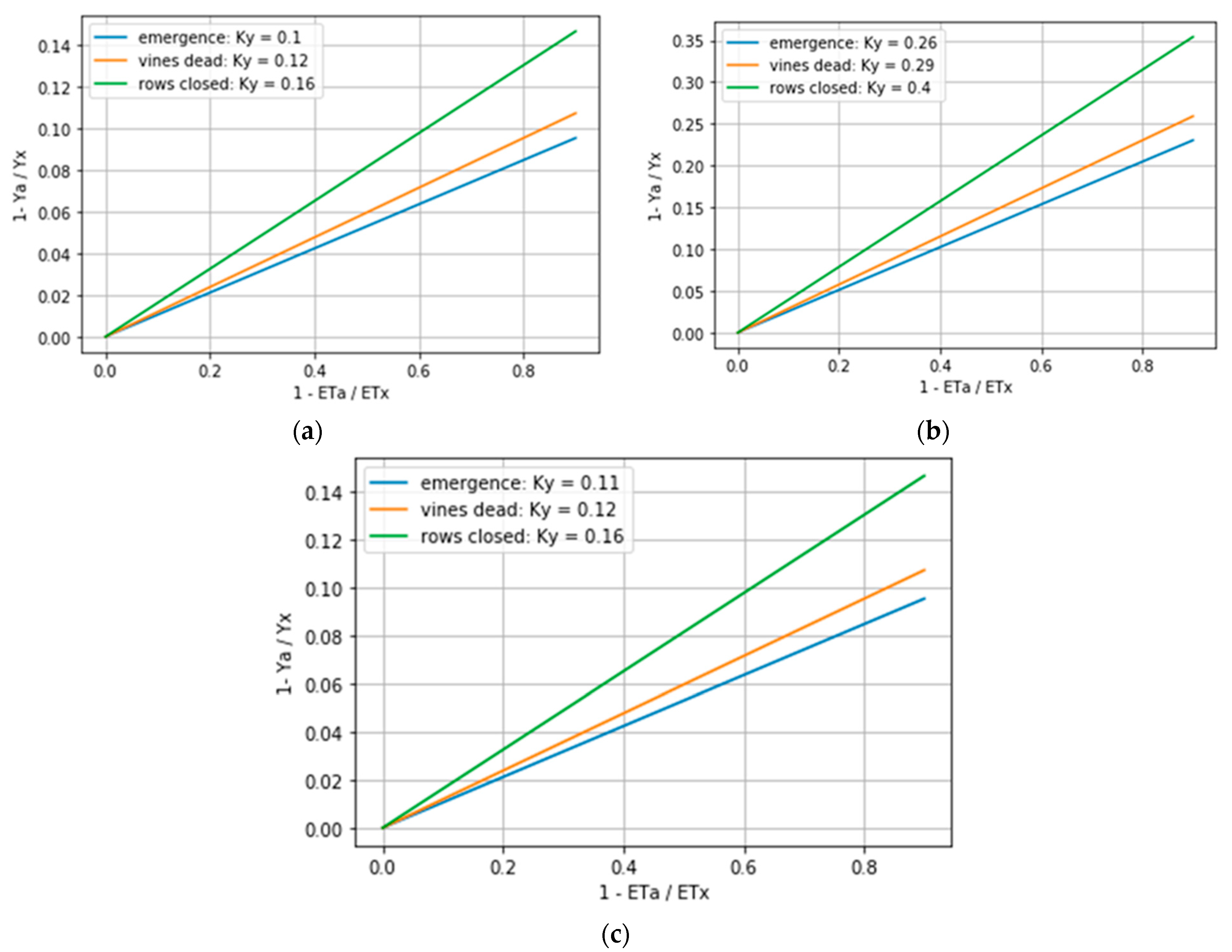
3.4. Crop Impact

This study performed a resilience study of an irrigation district in Southeastern Idaho, by setting up four different scenarios investigating the impact of low flow, unforeseen water demand increase, power outage and dam failure. System performance is selected as a measure of resilience, quantified by the ability of the system to meet demands, both in water and power. By applying these scenarios, we observed the system response, and implications, based on the interdependencies between the water and power systems. These scenarios would also have significant implications on irrigation needs and crop yields for farmers. Indeed, soil water availability is a major limiting factor in crop productivity [61,62]. Water deficits in crops, ultimately causing water stress, have an effect on crop evapotranspiration and crop yield. We illustrate the impacts of water stress on crop using scenario 1 (dry year) and scenario 3 (pump failure), as these address water stress. The relationship between crop yield and water use was established through a simple equation developed in the 70s [63]:

$$1-\frac{Y_a}{Y_x}=K_y \left(1-\frac{E{T}_a}{E{T}_x}\right)$$

(2)

where Y_x and Y_a are the maximum and actual yields, respectively, while ET_x and ET_a are the maximum and actual evapotranspiration (ET), and K_y is the yield response.

We consider potato crops in our example, given its prominence in the area. ET and crop data are gathered from AgriMet, which is a network composed of over 70 agricultural weather stations located throughout the Pacific Northwest [64]. Figure 13a,b display the linear functions for potato crops subjected to water deficits, in the case of scenario 3 presented in Section 3.3.3 with Trantham and Murphy pumps out, occurring during 3 growing stages, namely plant emergence, full cover (rows closed), and harvest (vines dead). The steeper the slope (i.e., the higher the K_y value), the greater the reduction in the yield for a given reduction in ET because of water deficits. The yield sensitivity to water stress varies over the growing season according to growth stages. Figure 15a shows that the stress occurring during the full cover phase has a limited impact in the case of Murphy, while, in the case of Trantham (Figure 15b), this phase is more sensitive to water stress. With a K_y < 1 in both cases, the crop is more tolerant to water deficits, exhibiting less than proportional reductions in yield with reduced water use [65]. However, the difference in impact of water stress at different stages can be seen, with a higher sensitivity to water deficit for the crop in the case of Trantham. While, for instance, a water use reduction at emergence stage for Trantham case of 40% may lead to 10% of yield reduction, the same water use reduction for the Murphy case may lead to only a 4% yield reduction. Figure 15c shows the crop response from water stress in scenario 1 in a dry year and with a reduced water supply. We can observe a similarity in yield response with the Murphy case, as both scenarios show about the same amount of unmet water demand (~2%). The expectations of what the yield could be while water is fully delivered in comparison to water stress diverge with not only the crop growth stages, but also water stress severity. Such differences in expectation could carry financial implications; that is, loss in revenue for farmers [66].

4. Discussion and Conclusions

The purpose of this research is to explore the concept of irrigation district resilience as integrated water and power systems. Operations and interdependencies are analyzed, in the context of assessing impacts on the water system due to events originating in the power system, or the inverse. Using a multi-agent modeling approach, we captured both water and power system components, as well as their linkages, and the decision-making process underlying the system operations. The model presents a more functional oriented representation of both the power system and the water system, with detailed operation and co-management features with contingency components represented.

Through simulation scenarios, we examine the system resilience, via system performance, when subjected to drought water year, unforeseen water demand increases, power outage and dam failure. Key outcomes of this study were:

• Low flow year effects are mostly felt in the power system, with not only a potential reduction in thermoelectric generation due to cooling requirements, but also a shift in the energy mix. With a water supply reduction between 20% and 30%, power generated from hydro plants drops by about 20%, placing the burden on other energy supply sources.
• The overall system appears to be resilient despite an unexpected increase in water demand. The storage remains at about 86% of full capacity, 2.2 times that of the minimum level in the last decade.
• The dam and district pumps seem to present the most vulnerable points in the system, causing a substantial amount of unmet demand when disrupted, leading to a need for large imports of power, and ultimately costs.

There is still room for improvement in this study. First, there is the issue of data availability. The authors have worked closely with local stakeholders to obtain and process the best available datasets to integrate water and energy aspects. However, some important datasets were not available either in public online sources or in local databases. Examples include water and power demand data. Assumptions were therefore made for quantification. Secondly, there are limitations related to the implications on crops. These include proxy values for the crop coefficient factors. Third, the spatial resolution of the demand was based on pump station distribution. The authors assume a uniform farm demand repartition throughout the district, with supposed similar water demand per pump location. It should be noted, however, that different spatial granularity may have an impact on the results, and should thus be explored in future research.

Despite these limitations, this analysis, we argue, takes water–energy nexus analysis a step ahead and is intended to provide insights for policymakers on the implications of disturbances throughout an irrigation district system in a rural area. This is a means to help identify and develop opportunities to improve resilience in the water and power sectors through coordinated planning, investment, and operations, and thereby provide benefits to utilities, consumers, and the environment.

The model will be further extended to assess the effects of resilience strategy implementation in a municipal system. Besides existing system components, the model will include additional relevant components or management decision making. By including such features, the model will allow stakeholders to investigate the benefits of strategies and policy mechanisms to improve co-management with an integrated system approach in larger communities.

References

- Bukhary, S.; Batista, J.; Ahmad, S. An Analysis of Energy Consumption and the Use of Renewables for a Small Drinking Water Treatment Plant. Water 2020, 12, 28. [Google Scholar] [CrossRef] [Green Version]
- Smith, K.; Liu, S. Energy for conventional water supply and wastewater treatment in urban China: A review. Glob. Chall. 2017, 1, 1600016. [Google Scholar] [CrossRef]
- Van Vliet, M.T.; Wiberg, D.; Leduc, S.; Riahi, K. Power-generation system vulnerability and adaptation to changes in climate and water resources. Nat. Clim. Chang. 2016, 6, 375–380. [Google Scholar] [CrossRef]
- DeNooyer, T.A.; Peschel, J.M.; Zhang, Z.; Stillwell, A.S. Integrating water resources and power generation: The energy–water nexus in Illinois. Appl. Energy 2016, 162, 363–371. [Google Scholar] [CrossRef]
- Fabiola, R. How the nexus of water/food/energy can be seen with the perspective of people well being and the Italian BES framework. Agric. Agric. Sci. Procedia 2016, 8, 732–740. [Google Scholar] [CrossRef] [Green Version]
- Engström, R.E.; Howells, M.; Destouni, G.; Bhatt, V.; Bazilian, M.; Rogner, H.-H. Connecting the resource nexus to basic urban service provision–with a focus on water-energy interactions in New York City. Sustain. Cities Soc. 2017, 31, 83–94. [Google Scholar] [CrossRef]
- Minne, L.; Pandit, A.; Crittenden, J.C.; Begovic, M.M.; Kim, I.; Jeong, H.; James, J.-A.; Lu, Z.; Xu, M.; French, S. Energy and water interdependence, and their implications for urban areas. In Electrical Transmission Systems and Smart Grids; Springer: Berlin/Heidelberg, Germany, 2013; pp. 239–270. [Google Scholar]
- DOE. The Water-Energy Nexus: Challenges and Opportunities; Department of Energy: Washigton, DC, USA, 2014.
- Koech, R.; Langat, P. Improving Irrigation Water Use Efficiency: A Review of Advances, Challenges and Opportunities in the Australian Context. Water 2018, 10, 1771. [Google Scholar] [CrossRef] [Green Version]
- Luna, T.; Ribau, J.; Figueiredo, D.; Alves, R. Improving energy efficiency in water supply systems with pump scheduling optimization. J. Clean. Prod. 2019, 213, 342–356. [Google Scholar] [CrossRef]
- Mercedes Garcia, A.V.; López-Jiménez, P.A.; Sánchez-Romero, F.-J.; Pérez-Sánchez, M. Objectives, Keys and Results in the Water Networks to Reach the Sustainable Development Goals. Water 2021, 13, 1268. [Google Scholar] [CrossRef]
- Vincent, C.; Tidwell, B.M.; Zemlick, K. The Geographic Footprint of Electricity Use for Water Services in the Western U.S. Environ. Sci Technol. 2014, 15, 7. [Google Scholar]
- DHS. Fact Sheet: Executive Order (EO) 13636 Improving Critical Infrastructure Cybersecurity and Presidential Policy Directive (PPD) 21 Critical Infrastructure Security and Resilience; Cybersecurity & Infrastructure Security Agency: Washigton, DC, USA, 2013.
- Newell, B.; Marsh, D.M.; Sharma, D. Enhancing the resilience of the Australian national electricity market: Taking a systems approach in policy development. Ecol. Soc. 2011, 16, 15–36. [Google Scholar] [CrossRef] [Green Version]
- Payet-Burin, R.; Kromann, M.; Pereira-Cardenal, S.; Strzepek, K.M.; Bauer-Gottwein, P. WHAT-IF: An open-source decision support tool for water infrastructure investment planning within the water–energy–food–climate nexus. Hydrol. Earth Syst. Sci. 2019, 23, 4129–4152. [Google Scholar] [CrossRef] [Green Version]
- Vinca, A.; Parkinson, S.; Byers, E.; Burek, P.; Khan, Z.; Krey, V.; Diuana, F.A.; Wang, Y.; Ilyas, A.; Köberle, A.C. The NExus Solutions Tool (NEST) v1. 0: An open platform for optimizing multi-scale energy–water–land system transformations. Geosci. Model Dev. 2020, 13, 1095–1121. [Google Scholar] [CrossRef] [Green Version]
- Saif, Y.; Almansoori, A. An optimization framework for the climate, land, energy, and water (CLEWs) nexus by a discrete optimization model. Energy Procedia 2017, 105, 3232–3238. [Google Scholar] [CrossRef]
- Almulla, Y.; Ramirez, C.; Pegios, K.; Korkovelos, A.; Strasser, L.D.; Lipponen, A.; Howells, M. A GIS-based approach to inform agriculture-water-energy nexus planning in the North Western Sahara Aquifer System (NWSAS). Sustainability 2020, 12, 7043. [Google Scholar] [CrossRef]
- Oikonomou, K.; Parvania, M.; Khatami, R. Optimal demand response scheduling for water distribution systems. IEEE Trans. Ind. Inform. 2018, 14, 5112–5122. [Google Scholar] [CrossRef]
- Oikonomou, K.; Parvania, M.; Burian, S. Integrating water distribution energy flexibility in power systems operation. In Proceedings of the 2017 IEEE Power & Energy Society General Meeting, Chicago, IL, USA, 16–20 July 2017; pp. 1–5. [Google Scholar]
- Qin, Y.; Curmi, E.; Kopec, G.M.; Allwood, J.M.; Richards, K.S. China’s energy-water nexus–assessment of the energy sector’s compliance with the “3 Red Lines” industrial water policy. Energy Policy 2015, 82, 131–143. [Google Scholar] [CrossRef] [Green Version]
- Dubreuil, A.; Assoumou, E.; Bouckaert, S.; Selosse, S.; Maı, N. Water modeling in an energy optimization framework–The water-scarce middle east context. Appl. Energy 2013, 101, 268–279. [Google Scholar] [CrossRef]
- Rieger, C.G. Resilient control systems practical metrics basis for defining mission impact. In Proceedings of the 2014 7th International Symposium on Resilient Control Systems (ISRCS), Denver, CO, USA, 19–21 August 2014; pp. 1–10. [Google Scholar]
- McJunkin, T.R.; Rieger, C.G. Electricity distribution system resilient control system metrics. In Proceedings of the 2017 Resilience Week (RWS), Wilmington, DE, USA, 18–22 September 2017; pp. 103–112. [Google Scholar]
- Vaagensmith, B.; McJunkin, T.; Vedros, K.; Reeves, J.; Wayment, J.; Boire, L.; Rieger, C.; Case, J. An integrated approach to improving power grid reliability: Merging of probabilistic risk assessment with resilience metrics. In Proceedings of the 2018 Resilience Week (RWS), Denver, CO, USA, 20–23 August 2018; pp. 139–146. [Google Scholar]
- Shinozuka, M.; Chang, S.E.; Cheng, T.-C.; Feng, M.; O’rourke, T.D.; Saadeghvaziri, M.A.; Dong, X.; Jin, X.; Wang, Y.; Shi, P. Resilience of Integrated Power and Water Systems; Citeseer: Berkeley, CA, USA, 2004. [Google Scholar]
- Simonovic, S.P.; Arunkumar, R. Comparison of static and dynamic resilience for a multipurpose reservoir operation. Water Resour. Res. 2016, 52, 8630–8649. [Google Scholar] [CrossRef]
- Akplogan, M.; Quesnel, G.; Garcia, F.; Joannon, A.; Martin-Clouaire, R. Towards a deliberative agent system based on DEVS formalism for application in agriculture. In Proceedings of the 2010 Summer Computer Simulation Conference, Ottawa, ON, Canada, 11–14 July 2010; pp. 250–257. [Google Scholar]
- Xiao, H.; Cao, M. Balancing the demand and supply of a power grid system via reliability modeling and maintenance optimization. Energy 2020, 210, 118470. [Google Scholar] [CrossRef]
- Walmsley, N.; Pearce, G. Towards sustainable water resources management: Bringing the Strategic Approach up-to-date. Irrig. Drain. Syst. 2010, 24, 191–203. [Google Scholar] [CrossRef]
- BPA. BPA Balancing Authority Load and Total Wind, Hydro, Fossil/Biomass, Nuclear Generation, and Net Interchange, Near-Real-Time. 2021. Available online: https://transmission.bpa.gov/Business/Operations/Wind/baltwg3.aspx (accessed on 10 August 2021).
- BoR. MID Facilities GIS Map; Bureau of Reclamation: Rupert, ID, USA, 2020. [Google Scholar]
- MID. Water Master Report for Minidoka Irrigation District 2019; Minidoka Irrigation District: Rupert, ID, USA, 2019.
- WU. Weather Underground. 2021. Available online: https://www.wunderground.com/ (accessed on 10 August 2021).
- Stene, E.A. The Minidoka Project; United States Bureau of Reclamation: Rupert, ID, USA, 1997. [Google Scholar]
- US Census. 2019 U.S. Population Estimates Continue to Show the Nation’s Growth Is Slowing. Available online: https://www.census.gov/newsroom/press-releases/2019/popest-nation.html (accessed on 10 August 2021).
- US Census. Resident Population Data. 2010. Available online: http://2010.census.gov/2010census/data/apportionment-pop-text.php (accessed on 10 August 2021).
- Kenny, J.F.; Barber, N.L.; Hutson, S.S.; Linsey, K.S.; Lovelace, J.K.; Maupin, M.A. Estimated Use of Water in the United States in 2005; US Geological Survey: Reston, VA, USA, 2009.
- USBoR. AgriMet Station Locations and Links to Homepages. Available online: https://www.usbr.gov/pn/agrimet/location.html (accessed on 10 August 2021).
- BoR. Hydromet Historical Data Access: Site Selection. 2020. Available online: https://www.usbr.gov/pn/hydromet/arcread.html (accessed on 10 August 2021).
- BoR. Minidoka Powerplant Minidoka Project; Bureau of Reclamation: Washington, DC, USA, 2007.
- Sargent, R.G. Verification and validation of simulation models. In Proceedings of the 2010 Winter Simulation Conference, Baltimore, MD, USA, 5–8 December 2010; pp. 166–183. [Google Scholar]
- Howard, G.; Bartram, J. The resilience of water supply and sanitation in the face of climate change Technical report. Who Vis. 2010, 2030, 42. [Google Scholar]
- NIDIS. Drought Conditions for Minidoka County. 2021. Available online: https://www.drought.gov/states/idaho/county/minidoka (accessed on 10 August 2021).
- Drastig, K.; Prochnow, A.; Libra, J.; Koch, H.; Rolinski, S. Irrigation water demand of selected agricultural crops in Germany between 1902 and 2010. Sci. Total Environ. 2016, 569, 1299–1314. [Google Scholar] [CrossRef] [PubMed]
- Heising, C. IEEE Recommended Practice for the Design of Reliable Industrial and Commercial Power Systems; IEEE Inc.: New York, NY, USA, 2007. [Google Scholar]
- Evans, B. Willing to Pay but Unwilling to Charge: Do Willingness to Pay Studies Make a Difference? University of Leeds: Leeds, UK, 1999; pp. 1–8. [Google Scholar]
- Vairavamoorthy, K.; Gorantiwar, S.D.; Pathirana, A. Managing urban water supplies in developing countries–Climate change and water scarcity scenarios. Phys. Chem. Earth Parts A/B/C 2008, 33, 330–339. [Google Scholar] [CrossRef]
- Sovacool, B.K.; Gilbert, A. Developing adaptive and integrated strategies for managing the electricity-water nexus. U. Rich. L. Rev. 2013, 48, 997. [Google Scholar]
- BoR. Water Year Graph. Available online: https://www.usbr.gov/pn/hydromet/wygraph.html?list=min%20af&daily=min%20af (accessed on 24 August 2021).
- BoR. Bureau of Reclamation, Pacific Northwest Region Major Storage Reservoirs in the Upper Snake River Basin. 2021. Available online: https://www.usbr.gov/pn/hydromet/burtea.html (accessed on 10 August 2021).
- NIDIS. DATA & MAPS: Historical Data and Conditions. 2021. Available online: https://www.drought.gov/historical-information# (accessed on 10 August 2021).
- Munger, D. Economic Consequences Methodology for Dam Failure Scenarios; Bureau of Reclamation: Washington, DC, USA, 2009.
- EIA. Electric Generator Dispatch Depends on System Demand and the Relative Cost of Operation. 2012. Available online: https://www.eia.gov/todayinenergy/detail.php?id=7590 (accessed on 15 August 2021).
- IRENA. Renewable Power Generation Costs in 2017. Available online: https://www.irena.org/publications/2018/jan/renewable-power-generation-costs-in-2017 (accessed on 1 January 2018).
- EIA. Electricity Explained: Factors Affecting Electricity Prices. Energy Information Agency, 2020. Available online: https://www.eia.gov/energyexplained/electricity/prices-and-factors-affecting-prices.php (accessed on 1 August 2021).
- DOE. 4 Reasons Why Hydropower is the Guardian of the Grid. Department of Energy, 2017. Available online: https://www.energy.gov/eere/articles/4-reasons-why-hydropower-guardian-grid#:~:text=Hydropower%20is%20an%20extremely%20flexible,and%20frequencies%20across%20the%20grid (accessed on 1 August 2021).
- Hell, J. High flexible Hydropower Generation concepts for future grids. J. Phys. Conf. Ser. 2017, 813, 012007. [Google Scholar] [CrossRef] [Green Version]
- Tahseen, S.; Karney, B.W. Reviewing and critiquing published approaches to the sustainability assessment of hydropower. Renew. Sustain. Energy Rev. 2017, 67, 225–234. [Google Scholar] [CrossRef]
- Denholm, P.; Hand, M. Grid flexibility and storage required to achieve very high penetration of variable renewable electricity. Energy Policy 2011, 39, 1817–1830. [Google Scholar] [CrossRef]
- Greaves, G.E.; Wang, Y.-M. Yield response, water productivity, and seasonal water production functions for maize under deficit irrigation water management in southern Taiwan. Plant Prod. Sci. 2017, 20, 353–365. [Google Scholar] [CrossRef] [Green Version]
- Lovelli, S.; Perniola, M.; Ferrara, A.; Di Tommaso, T. Yield response factor to water (Ky) and water use efficiency of Carthamus tinctorius L. and Solanum melongena L. Agric. Water Manag. 2007, 92, 73–80. [Google Scholar] [CrossRef]
- Smith, M.; Steduto, P. Yield response to water: The original FAO water production function. Fao Irrig. Drain. Pap. 2012, 6–13. [Google Scholar]
- BoR. AgriMet: Cooperative Agricultural Weather Network. 2016. Available online: https://www.usbr.gov/pn/agrimet/general.html (accessed on 10 August 2021).
- Steduto, P.; Hsiao, T.C.; Fereres, E.; Raes, D. Crop Yield Response to Water; Food and Agriculture Organization of the United Nations: Rome, Italy, 2012; Volume 1028. [Google Scholar]
- DiGiacomo, G.; Hadrich, J.; Hutchison, W.D.; Peterson, H.; Rogers, M. Economic Impact of Spotted Wing Drosophila (Diptera: Drosophilidae) Yield Loss on Minnesota Raspberry Farms: A Grower Survey. J. Integr. Pest Manag. 2019, 10, 11. [Google Scholar] [CrossRef] [Green Version]