Smart City Taxi Trajectory Coverage and Capacity Evaluation Model for Vehicular Sensor Networks

Abstract

In a smart city, a large number of smart sensors are operating and creating a large amount of data for a large number of applications. Collecting data from these sensors poses some challenges, such as the connectivity of the sensors to the data center through the communication network, which in turn requires expensive infrastructure. The delay-tolerant networks are of interest to connect smart sensors at a large scale with their data centers through the smart vehicles (e.g., transport fleets or taxi cabs) due to a number of virtues such as data offloading, operations, and communication on asymmetric links. In this article, we analyze the coverage and capacity of vehicular sensor networks for data dissemination between smart sensors and their data centers using delay-tolerant networks. Therein, we observed the temporal and spatial movement of vehicles in a very large coverage area (25 × 25 km${}^2$) in Beijing. Our algorithm sorts the entire city into different rectangular grids of various sizes and calculates the possible chances of contact between smart sensors and taxis. We further calculate the vehicle density, coverage, and capacity of each grid through a real-time taxi trajectory. In our proposed study, numerical and spatial mining show that even with a relatively small subset of vehicles (100 to 400) in a smart city, the potential for data dissemination is as high as several petabytes. Our proposed network can use different cell sizes and various wireless technologies to achieve significant network area coverage. When the cell size is greater than 500 m${}^2$, we observe a coverage rate of 90% every day. Our findings prove that the proposed network model is suitable for those systems that can tolerate delays and have large data dissemination networks since the performance is insensitive to the delay with high data offloading capacity.

1. Introduction

Smart urbanization will soon significantly improve our lifestyle by enabling communication technologies and plenty of Internet-of-Things (IoT) applications like smart homes, smart vehicles, smart grids, eHealth, and much more. Therein, smart sensors can play a vital role to observe different environmental variables, disseminate their data, and provide in-time actions based on advanced big data analytics. These smart sensors can ubiquitously discover their spaces in a wide scope of IoT applications due to their low cost, small size, and ease of deployment. There are a number of applications where smart sensors can be plugged into the IoT devices to improve their functionality or productivity, e.g., climate observations, waste management, traffic surveillance, safety and security, etc. However, there exists two key challenges in this regard [1], which include power management and data dissemination to/from administrative bodies of the sensors.

The power management and communication network for sensor data are depending on the cost and quality of communication requirements. For instance, real-time communication requires expensive infrastructure over all nodes that could be very expensive. To this end, we need a ubiquitous and reliable communication infrastructure such as conventional networks, or cellular networks. However, the conventional networks or cellular systems could not be adequate to fulfill the requirements such that they may fail to provide connectivity under the peak load [1]. Moreover, connecting a massive number of smart sensors to a conventional network or some other IP based traditional network may look insignificant technically. It is problematic from both administrative and economic point of view to instal a SIM card on each sensor. It is also unrealistic for the management of sensor gateways or femtocells in the entire city under the same administration.

Software updates in smart vehicles do not require real-time communication, because opportunistic and D2D technology have advantages, but there are compromises in terms of packet delay. The Vehicle Delay Tolerance Network (VDTN) can be used to forward and deliver software update packages in a store-carry-forward manner. In return, it not only saves costs and energy, but also offloads cellular traffic. In addition, VDTN’s architecture can implement location-based and point-to-point services, so it may be more suitable for many vehicle-related use cases. In this regard, data services for games, audio and video streaming may also be useful among vehicle users, such as social networks in vehicular proximity [2]. Traditionally, such applications are maintained by LTE-direct, WiFi-direct, or DSRC communication technology. However, the long pairing time (between devices) and data packet collisions in these technologies may not meet the requirements of smart cities. Therefore, the application of VDTN is a good candidate solution for disseminating data to smart sensors in in-vehicle networks.

We can use the VTDN architecture in the taxicab fleet of a smart city as an alternative channel of communication to reduce the load on conventional networks or cellular networks [3]. In [4,5], the authors use the annual average daily traffic of Auckland city and perform theoretical and mathematical analysis to calculate data transmission delays in smart cities. We can find a detailed framework of this system in [6]. In this paper, we explore the collection of big data produced by a massive number of smart devices using vehicular sensor networks as an alternate data dissemination channel. We may piggyback accumulated data on moving taxi-cabs for data delivery at data centers of the corresponding service by using the opportunistic contacts between the sensors and the microscopic movement of vehicles with their Global Positioning System (GPS) location information. This will not only reduce the load on expensive cellular links, but also eliminates the need for new infrastructure deployment.

In this paper, we focused on the data collection of smart sensors deployed at various locations of the smart city through the vehicular networks and evaluated potential locations for data transmission, network coverage, and capacity. The ubiquitous availability and displacement of taxi cabs can help us in data collection and disseminate the collected data throughout the smart city. However, we must consider that these taxi-cabs can cooperatively deliver the essential coverage and capacity to serve the purpose. In this regard, we analyze the coverage and capacity of the intelligent sensing system of vehicles by considering the possible contacts of taxicabs in different locations. We used the real-time taxi traces of Beijing city in order to evaluate the proposed model. Therein, we cut the complexity of the network by using a grid clustering algorithm on big data of taxi traces. In our model, the cluster is a rectangular region from where a vehicle can collect or deliver data. Moreover, we apply different spatial data mining techniques to filter the data and analyze it for different wireless technologies by using the different sizes of clusters. We investigated the data dissemination of vehicular sensor networks in smart cities, which can help network engineers configure the network to obtain good coverage and capacity. The analysis of this work can help designers design a system to support the city government to manage data from various data sources, such as smart sensors, video surveillance cameras, and smart city control centers.

The key contributions of this paper are summarized as follows:

• We propose an smart city model for data collection of densely deployed devices, which saves a huge amount of cost for infrastructure deployment. We propose a grid clustering algorithm in order to reduce the complexity of data analysis and observe network dynamics. Our algorithm logically divides the whole city in different sizes of clusters to identify opportunistic contacts between smart vehicles and to figure out the vehicle density in each cluster.
• We applied our proposed algorithms on real taxi traces of the Beijing city to analyze the network coverage and capacity of the proposed network model. Therein, we observed that a huge amount of data can be disseminated by using our proposed model with high coverage. This network model can collect more than 100 TB data and provide 98% coverage per day under IEEE 802.11p standard.
• We develop a greedy algorithm for Roadside Units (RSU) placement in a smart city to identify the most popular locations in terms of the highest number of opportunistic contacts of smart vehicles with smart sensors. We analyze our proposed network of vehicles for data transmission service scenario from the service provider to smart sensors using software update code.

The rest of this paper is organized as follows. Section 2 provides a summary of the related work. Section 3 describes an overview of the proposed network model. Section 4 presents the evaluation of the proposed model and discusses the results. Some limitations of this study are discussed in Section 5. Finally, we conclude the paper in the last section.

2. Related Work

We here discuss the summary of the research works related to our study in the following.

2.1. Data Mules

Data mules have been used for the sensor networks to deal with the cost of energy consumption issues in the short-range wireless communication technologies. Therein, the mobile node can forward data to other nodes by the store-carry-forward approach as that in mobile ad hoc networks [7]. There exist different studies on data mule mobility in the literature to evaluate the performance of data collection in various applications. For example, the random motion of mobile nodes is considered in 2D-rectangular area [8]. We can find related studies in [9,10], therein the author have used displacement of data mules. In [11], authors exploit mobility prediction of data mules and use message farriers in sparse sensor networks for proactive data delivery. The controlling and planning of data mules mobility is testified in [12,13,14] and uses various optimization techniques in complex problems of data forwarding with optimal and sub-optimal techniques [15,16,17,18,19]. In the existing literature, authors focused on the data forwarding capacity of vehicular networks by considering the diverse type of vehicles having a specific type of wireless communication technology along with controlled movement and mobility prediction of the vehicles. Therein, the typical mobility of the taxi is considered uniform in terms of velocity or spatially, which is an unrealistic assumption. We consider the sparse displacement and uncontrolled movement of vehicles as data mules moving in the entire city. Moreover, we do not consider specific wireless technology in our analysis. Here we consider the wireless coverage range as an input variable that is generic and adjustable to various types of applications in smart cities.

2.2. Opportunistic Communication in VTDNs

In [20], the VTDNs are used to sense data from a smart city environment to assist traffic management, navigation, and pollution control. Some research works show the collaboration of vehicular networks with wireless sensor networks in smart cities. In [21], optimal placement of the smart sensor is investigated along the roadside to get optimal coverage for navigation support. Driving safely applications are described and studied in [22]. A few other research works describe the potential of different technologies in different case scenarios of vehicular networks [23,24,25,26,27]. In [20], vehicular networks are used to sense data from a smart city environment to assist traffic management, navigation, and pollution control. In [21], optimal placement of the smart sensor is investigated along the roadside to get optimal coverage for navigation support. Driving safely applications are studied in [22]. In [28], the authors used the road network for data forwarding and propose an alternate offloading channel. They consider the vehicle mobility at France roads to transport big data from 250 GB to 1TB by each vehicle. Therein, the results show that in 3 h, more than 260 terabytes of data can be disseminated, which is 200 times higher than that of the traditional network. In [29], the authors investigated a hypothetical network of shared bikes. The bikes can communicate with each other and with different bike stations in the given scenario. A motorbike can transfer up to twelve-gigabyte data on a trip. However, the traffic fluctuation shows that in the selected area the coverage is not uniform. In [30], authors demonstrate the opportunistic network of boats having access points of IEEE 802.11g at the Amazon Basin. Their evaluation shows that the boat network can disseminate up to 1TB per week. We can find different types of vehicles that as in [28,29,30], which conclude that terabytes of data can be disseminated in different scenarios. In this connection, still there exists a huge research gap to accommodate the big data of smart sensors in vehicular networks. In our work, we use a big data set of real-time traces of taxicabs and identify the potential locations for data transmission in Beijing city to figure out the quantity of data dissemination.

2.3. Vehicle Traces

The performance of vehicular networks can be evaluated under the two types of methods. First, evaluating the performance with the network simulator. In this regard, IMPORTANT is one of the earliest simulators of mobile ad hoc networks [31]. This framework has several mobility models including the grid-based Manhattan vehicle mobility model to evaluate the performance of different routing protocols. The authors pointed out several limitations that this framework neglects geographical, temporal, and spatial dependencies of moving vehicles [cite here]. VanetMobiSim [32] is another simulator for vehicle mobility. This is a more realistic simulator to simulate scenarios near to reality because it supports many parameters like differentiated speed, multi-lane roads, traffic signs at intersections, and separate flow in both directions. Researchers have developed another integrated set of tools called TRANSIM to analyze the regional public transportation systems [33], which includes several vehicle mobility aspects of cellular automata to evaluate connectivity among vehicles. SUMO [34] is an open-source simulator that uses the GIPPS model for traffic flow simulation. It contains a wide range of parameter settings including traffic lights.

On the other hand, analyzing the vehicle movement in the selected area by using vehicle traces is an alternate solution. There exist two types of vehicle traces in the literature including synthetic traces created by some scientific model and the real traces collected by GPS locations of the mobile vehicles. In model-based traces, an area is usually chosen from a city with the mapping of traffic signs and streets to be evaluated with a synthetic mathematical motion model for a selected time interval [35]. Therein, the selection of parameters like mobility model, number of cars, typologies, vehicle speed are not optimal. Moreover, these traces are limited to a few km${}^2$ areas and having short time intervals [36]. A mobility model should consider several parameters for real mobility (e.g., traffic lights, weather conditions, one-way or two-way streets, driving behaviors, obstacles, etc.). However, it makes a model much more complex. The real-world traces can be recorded by collecting the GPS position of mobile vehicles. Collecting GPS data of all vehicles displaced in the entire city is not easy for different reasons, like privacy issues of the drivers, and not all of the vehicles are equipped with the GPS system. So, this data can be obtained by a vehicle fleet company like a taxicab fleet [37].

The authors in [38,39] evaluate the network performance of vehicular networks with real-time traces [40]. In this regard, mostly the used trace data is available publicly. For example, the GPS trace data of 13,799 taxis for 9 days in Shenzhen, China, 533 taxis GPS data of 20 days from San Francisco, USA, and 320 taxi cabs data from the city of Rome. In our work, we evaluated and analyzed the GPS data of taxi cabs in Beijing, China because its topology is different than that of the others. The road topology and traffic conditions in Beijing are entirely different from synthetic traces generated by simulators. The real-world GPS traces of vehicles’ databases collected from Shenzhen, Rome, and San Francisco are also not suitable to our scenario because they have simple topological assumptions [41,42,43]. In [44], the authors use GPS data of 16,000 taxicabs and evaluated traffic visualization, urban planning, and analysis in Singapore city. Their work is on different parameters of smart cities rather than opportunistic communication of vehicles with smart sensors. However, this work validates that taxi displacement is promptly converging, which means that the random destination of different passengers and taxis will visit the random location of the city, and so it leads to high coverage. This is simply an affirmation of our vehicle-based application that speaks in support of our scenario.

3. Proposed Smart City Model

We proposed an alternate data collection network model to collect delay tolerant data from densely deployed Smart Sensors (SSs) in a smart city as shown in Figure 1. The main components of our proposed network are smart vehicles, Roadside Units (RSUs), Central Controller (CC), Control Units (CUs), and Data Sources (DSs), e.g., SSs. We use smart vehicles for the collection of data from data sources and transmit to data centers of their controlling bodies. Similarly, these vehicles can also be used to transfer software update code from controlling bodies to SSs. The CC will govern overall communication between DSs and CUs with the help of three different networks, e.g., cellular network, traditional network or our proposed vehicular network. A few examples of the controlling bodies of smart city services are also shown in the bottom of the figure.

In cities, the wireless transmission coverage of cellular systems is ubiquitous. Therefore, we assume that different data sources and SSs are installed in different types of structures to collect status data for various applications in a smart city. Therein, the intelligent vehicle drives on the road through the interface of WiFi, GPS and cellular technology. In addition, smart vehicles have data storage capabilities and processing capabilities, so they can easily form a network with RSU as a Base Station (BS) through a cellular interface or with other connected vehicles through a WiFi interface. A CC server is connected at the cellular network to manage the overall communication. Since the smart devices generate a huge volume of data in the city, so the CC server selects the traditional core network or cellular network or, our proposed vehicular network to forward the delay-sensitive data.

Whenever a data source needs to send information to a CU or a Data Center (DC), it sends a data packet containing an information request to the CC server on the cellular control channel. In return, CC will select the most suitable network to serve the purpose. The decision of network selection is made by considering many parameters such as the number of vehicles on the road, the delay tolerance interval, the history of the vehicle route, and the cost of energy. In this regard, if the infrastructure network is more suitable for a given parameter set, then CC recommends that the source send data on the suggested path, i.e., path (a) or path (b), as shown in Figure 1. The data can be forwarded and transmitted through the vehicle transport network on path (c) otherwise. The CC server selects the optimal number of vehicles based on the historical information of the vehicle trajectory, and informs DS to transmit data through these vehicles, which are selected for specific data set requirements. Whenever the selected vehicles find the RSU through the WiFi interface, they will upload data on the receiving end. The RSU is linked to the city through the backbone network and sends data to the CU. Once the data is received, the RSU sends the acknowledgment message to the server.

If due to some kind of error, the data message is not received by the CU before the delay tolerance indicator expires, then such data will be directly transmitted to the CU using the cellular interface. Moreover, the vehicles in our proposed work are smart enough, and they can analyze the data collected from the sensors. If the data collected from the sensor needs to upload urgently, then smart vehicles can upload it by their cellular links.

Whenever a service provider at CU or DC wants to send data to SSs (e.g., in case of software update code), it sends the data request to the CC server. Finally, the CC server will use the proposed SC architecture to forward this data from a service provider to SSs by smart vehicles.

In the next sections, we explain how we can divide our selected area into different sizes of grids to calculate coverage and potential of our proposed SC architecture with respect to different wireless technologies.

3.1. Area Division

We consider the microscopic movement of the vehicles based on GPS locations and trajectory traces for data dissemination so as to analyze the network coverage and its potential. We, therefore, divide the whole city into smaller grids. A grid is a rectangular region bound by some longitude and latitude values. The length of each grid depends upon the chosen wireless technology. The number of vehicles reported inside a grid form a cluster.

We now describe the model to calculate the effective distance of a vehicle from a wireless device inside a grid in the following. Before we proceed, we have summarized the notations in

Table 1. Summary of symbols used.

Symbol	Description
d	Effective distance of a vehicle to a device
$d_0$	Reference distance of a vehicle
$n_0$	Path loss factor
$\Psi$	Gaussian random variable
$\rho$	Vehicle density
r	Length of each side of grid cluster
tid	Taxi id
Lon	Longitude
Lat	Latitude
aid	Cluster area ID
$S_i$	Size of wireless technology used
t	Unit time interval
m	Total number of clusters in $S_i$
n	Total number of GPS points in selected area (25 × 25 km${}^2$)
T	Average update time
$ST$	Stay time in a cluster
$\theta$	Data rate of wireless technology

, which are used to calculate the effective distance, cluster density, network area coverage, and network capacity, thereon.

3.2. Effective Distance

Whenever a vehicle will visit a rectangular grid cluster, it can collect data from all the devices inside that cluster. For this purpose, the size of the grid cluster will be adjusted for the selected wireless technology. The vehicle must be kept within the appropriate area of the wireless coverage area of the smart device to reduce packet loss, as shown in Figure 2. The path loss $PL\left(d\right)$ of a vehicle at a distance of d can be calculated by the path loss formula [45] as follows,

$$PL\left(d\right)\left[dB\right]=P{L}_F\left(d_0\right)+10n_{0}log\left(\frac{d}{d_0}\right)+\Psi ,$$

(1)

where $d_0$ is the reference distance (where path loss receives the characteristics of free-space loss, $P{L}_F$), $n_0$ represents the path loss index depending on the propagation environment. $\Psi$ stands for Gaussian random variable.

From Equation (1), we can calculate the effective distance from the vehicle to the wireless device in the grid as follows,

$$d=d_0\times {10}^{\frac{P{L}_F\left(d_0\right)+\Psi -PL}{10\left(n_0\right)}},$$

(2)

where d refers to the distance of a vehicle to a device. So, the effective distance will be $2d$ by considering the diameter of the wireless coverage area of the device. As shown in Figure 2, every smart vehicle can simply send data packets to a device at a distance of 0 to 2d meters.

We can divide the whole selected area to identify the presence of a vehicle in a given area. Each grid has a length of each side (denoted by r) as shown in Figure 2. If d is the radius of wireless coverage of a device, then the maximum length of wireless coverage can be calculated as follows,

$$2d=\sqrt{r^2+r^2},$$

(3)

where r is the length of each side of a grid topology. Equation (3) can be written as,

$$d=\frac{1}{\sqrt{2}}r,$$

(4)

So, the length of each side of grid can be calculated with the following,

$$r=\sqrt{2}\times d_0\times {10}^{\frac{P{L}_F\left(d_0\right)+\Psi -PL}{10\left(n_0\right)}},$$

(5)

As shown in Figure 2, if r is the length of each side of the grid, then any vehicle at a distance $\frac{1}{\sqrt{2}}r$ or double of it is in the wireless range of a device. Thus, it can can collect data from that device. We now describe our algorithm for this division related to different wireless technology.

3.3. Grid Clustering Algorithm

The cost to evaluate all possible taxicab encounters with geographically stationary sensors is high. Therefore, it is important to process data for every taxicab in the area characterized by the wireless coverage for all time intervals. For this situation, the databases of vehicle trajectories are of noteworthy size, so the procedure of complex mining is expensive and tedious. The data set is made out of GPS locations of taxicabs during the whole day’s intervals. There are various approaches to dissect huge measures of spatial data like sampling an array of GPS points, decreasing the investigated area, clustering, measuring the distance between all GPS locations to cite a few. However, we are interested to examine the reasonableness of wireless technology along with its range. So, we have used the grid clustering method because it garbs well our proposed study and problem.

We have proposed Algorithm 1 for grid clustering to reduce the complexity of big data analysis, which is inspired by the Statistical Information Grid Approach to Spatial Data Mining (STING) [46]. Our clustering algorithm gets input values as taxi ID, date time, location, starting value of longitude and latitude, and the set of the different wireless technologies coverage range to build rectangular and spatial clusters of different sizes according to given wireless ranges.

Algorithm 1: Grid clustering algorithm.

3.4. Cluster Density

The density of a grid with size $S_i$ is the number of records mapped or reported updates in that grid until a time t. it can be written as follows,

$$Density(S_i,t)=\left|M(S_i,t)\right|$$

(6)

We can calculate the sum of all densities of all clusters m in each time t as in the following,

$$M_{Density}\left(t\right)=\sum _{i=1}^m|M(S_i,t)|$$

(7)

We proposed Algorithm 2 to estimate vehicle density in each cluster area of size $S_i$, which is the number of vehicle visits in each cluster. A cluster that has more vehicle visits simply means a high dense cluster, while a low dense cluster means it has a smaller number of vehicle visits otherwise. More popular areas with high dense clusters have a high potential for data dissemination and so they can be used as a location for RSU installation.

Algorithm 2: Cluster density algorithm.

3.5. Network Area Coverage

If vehicles cover k clusters in time t, we can calculate percentage coverage with the following,

$$Coverage\left(S\right)=\sum _{i=1}^k\frac{S_i\times 100}{Tota{l}_{aid}}$$

(8)

We design Algorithm 3 to measure the coverage of clusters $S_i$ in our selected area by vehicle displacement in time T. The time T is divided into equal smaller intervals $t_i$ as $T=\{t_1,t_2,\hspace{1em},t_n\}$. Some areas where vehicles are not allowed to visit have zero coverage.

Algorithm 3: Area coverage algorithm.

3.6. Network Capacity

Network capacity is the total potential of our proposed architecture that defines how much data can be disseminated by considering all possible contacts in each cluster of our selected area. These contacts can be calculated by the displacement and movement of vehicles in different clusters of size $S_i$. By getting the total number of possible contacts (or updates), we can simply calculate the total stay time $ST$ of each vehicle in each cluster. Finally, the capacity of the network, with the data rate $\theta$ of each selected wireless technology in each cluster of size $S_i$ can be calculated as follows,

$$Capacity\left(S\right)=\theta \times T\times \sum _{i=1}^m|M(S_i,t)|$$

(9)

where T is the average update interval. We implement Equation (9) in Algorithm 4 to illustrate how we calculate network capacity. The inner for loop calculates the number of updates and stay time in each cluster of size $S_j$. The outer for loop calculates total stay time in all clusters of size $S_j$. Finally, the algorithm returns the network capacity with respect to data rate of selected wireless technology.

Algorithm 4: Network capacity algorithm.

3.7. RSU Placement

RSUs are directly attached to the CC server. In our proposed network, it is essential to deploy the RSUs at important locations. We can use RSUs to transfer data from a service provider to smart sensors because they have storage, processing, and communication capabilities. The service provider can send the data (e.g., software update) for sensors to the CC server that forwards this data to RSUs by using a traditional network (e.g., cellular network). So, vehicles can easily get the data from the RSUs and forward it to the SSs. In this regard, we consider the most visited locations of a geographical area visited by vehicles and used the greedy Algorithm 5 for the RSUs placement.

Algorithm 5: Greedy algorithm for RSU placement.

4. Performance Analysis

We use taxi trajectories data to calculate the coverage and capacity of on-board sensor networks in smart cities to calculate the stay time of vehicle in each grid, find the coverage, and data dissemination capabilities of the vehicular sensor network. For this purpose, we implement the vehicle big data traces in SQL Server to calculate the number of contacts between different smart sensors, roadside units and vehicles in different scale grids. We apply our proposed clustering algorithm to divide vehicle data into different clusters, and execute SQL queries in different scenarios of D2D communication and various wireless technologies to calculate various results that are helpful for smart city design and analysis. The most important part of the taxi fleet is the taxicabs that can reach each street at the exact destination/origin of the riders and can provide more excellent coverage. In this regard, we have selected four subsets of 400 random taxis from Beijing city having an average update time of 30 s. We evaluate the vehicle capacity, Cluster coverage, cluster density and performance of our proposed vehicular network for data collection. We here briefly describe the data set, locations with high potential for data transmission, coverage, and capacity of the proposed network.

4.1. Beijing Taxi Traces Overview

Taxi traces of Beijing city are available at the Microsoft repository as a T-Drive data set by MSRA [47]. This data set contains the information of 10,375 taxi trajectories, having the GPS positions of taxis in the most populated and congested city of Beijing. The total number of GPS updates in this data set reaches 15 million points, and these taxi trajectories cover a distance up to 9 million kilometers. Figure 3 shows the visual representation of these traces for one day. The heat map colors represent the different densities of taxis on Monday (4 February 2008). We draw the heat map by using a MATLAB function Scatter Plot colored by Kernel Density Estimate to calculate the vehicle density to each GPS location [48]. We can see that it is difficult to analyze each possible contact in a selected geographical area, so we used our grid clustering algorithm to reduce the complexity and calculated the possible contacts in each clustered area rather than at each GPS location. The average update time in this data set is 177 s. The average distance between the consecutive points is 623 m. The average speed of the taxis in these traces is 12.67 km/h nearly equal to 7.5 miles/h, which is validated at [49]. This implies that these distinct points have enough data to represent the persistent trajectories of taxicabs [50,51]. Each text file of this repository, name by the ID of the taxi, contains the geographical information of each taxicab.

4.2. Area Selection for Analysis

We selected an area of 25 × 25 km${}^2$ having longitude between $116.{24}^{°}$ E to $116.{5335}^{°}$ E and latitude between $39.{8125}^{°}$ N to $40.{04}^{°}$ N to evaluate the network performance, coverage, and capacity. The initial step of our methodology is to apply the grid clustering algorithm on taxi traces to make a graph having every vertex as a geographic area of the selected city called a grid. Every vertex has a weight that is equivalent to the total number of taxicabs reported inside that grid. After the creation of grids, the whole area is separated into equivalent measured quadrants. Finally, the GPS locations of each taxi are stored in the database, along with their quadrants (grids) as shown in Figure 4. A grid is a small region of the city bound by a square with a side length r demarcated by GPS locations of taxis. If n is the total number of GPS points, then during the association phase, our algorithm has $O\left(n\right)$ complexity. This complexity condensed to $O\left(m\right)$ at higher levels, where m is the total number of grids in the target region. Additionally, this is the basic advantage of the grid clustering algorithm because it has less complexity, i.e., $m<<n$.

It is crucial to choose the grid size judicially. The grid size should be neither too big nor too small, which influences the performance of our proposed work directly for evaluation of radio ranges of chosen wireless technologies. We analyze the coverage and dynamics of the proposed network by using the four random subsets of 100, 200, 300, and 400 taxi cabs from the data set of Beijing Taxi traces by considering the wireless range of different wireless technologies as shown in

Table 2. Selection of cluster size with a coverage range of different wireless technologies.

ID	Cell Size	Area	Total Cells	Lon. Inc.	Lat. Inc.	Wireless Technology
1	1000 m	25 × 25	625	0.0174	0.008992	IEEE 802.11p
2	500 m	50 × 50	2500	0.00587	0.004496	IEEE 802.16
3	250 m	250 × 250	10,000	0.002935	0.002248	IEEE 802.11n
4	100 m	100 × 100	62,500	0.001174	0.008992	IEEE 802.11ay

.

4.3. Vehicle Density

It is important to stop at each desired layer of Algorithm 1 to evaluate the network dynamics, where the size of the layered grid matches with the radio range of wireless technology. Based on this division, we got a heatmap table of 400 cabs visits in each grid of 1000 m${}^2$ size as shown in Figure 4. The colors of the heat table show the vehicle density of cabs in all grids. The cab density varies from yellow grid 0% to the darkest grid of 94.5%. The GPS locations having a great human index have more cab visits. More vehicles’ visits in a grid mean more chance to transfer or receive data from sensors to vehicles in that grid. The maximum degree of a grid is 378, and the average degree of a grid is 166. The percentage of grids having a degree greater than the average value is 48.16%. Having an average degree of 166 means that the network is highly connected. The connectivity of the proposed network can be illustrated by quantifying the displacement of taxi cabs in the city during some specific periods. By analyzing GPS locations, it is promising to categorize patterns that are distinctive of the transportation networks in Beijing. By this analysis, we can find the areas or grids where taxicabs stay a longer period of time. These can be taxi stops or highly congested areas. One of the main objective of this work is identifying the locations with a high potential for data transmission. Hence, clusters having high density have a high potential for data dissemination.

4.4. Network Area Coverage

We evaluate the percentage of grid coverage of 1000 m${}^2$ by using a set of 400 random vehicles for a given interval. Figure 5 compares the grid coverage percentage of a working day, a weekend day, and the weekly average. In all three cases, there is a big coverage of the area, which has area coverage around 95% after a half-day. Some of the grids can never be visited, e.g., the grid with ID 27. So, the coverage can never be 100% under this given case.

Figure 6 shows the area coverage by the displacement of 400 random taxi cabs of the given data set in 24 h. In this experiment, we investigate the coverage for different grid sizes that varies from 100 m${}^2$ to 1 km${}^2$. In the case of 1 km${}^2$ grid size, the coverage of the area varies from 80% to 98.5%. Almost 1.5% of the grids can never be visited by these cabs. By geographical inspection of the selected area, it is observed that these grids are in the regions where taxi cabs and vehicle movement is not allowed, e.g., old cemeteries, big private areas, public gardens, train stations, rivers, hotels, etc. As shown in Figure 6, the coverage of the area reduces when we reduce the size of the grids from 500 m${}^2$ to 250 m${}^2$ and 100 m${}^2$. The smallest grid size division is 100 m${}^2$, which gives the smaller coverage that varies from 10% to 30% in 24 h. The average road area in Beijing city is 26% [52]. In this division, we noticed that only those grids are covered that are on the road or near the coverage of the road. All the smaller grids that are away from the road can never send their data directly to the vehicles because they are not in the wireless range of the vehicles having the technology of 100 m${}^2$ wireless range. However, these areas can also be covered if we use the clustering approach of wireless sensor networks. All the sensors away from the road will then route their accumulated data to their cluster heads periodically. These cluster heads are installed in those grids, which are in the coverage of some road.

Figure 7 shows the coverage of the given area with a different number of taxi cab sets in 24 h on 4 February 2008. This experiment shows that when we increase the number of vehicles, the coverage also goes on increasing. The subset of 100 taxicabs gives coverage from 60% to 92% of the given area, whereas the bigger set having 400 random cabs give higher coverage from 80% to 98.5% of the given area. We would like to mention that the focus of our investigation was an urban region of $25\times 25$ km${}^2$ area. However, this situation may not necessarily apply in hardly populated regions or rural areas. In this connection, we think that the locations where more taxicabs move, frequently compared to locations where more information is produced/consumed, and at those locations, the data dissemination is usually progressively critical. This reflection is true likewise if we consider the different regions of the same city. Furthermore, on the off chance that we consider for example uncommon occasions like domestic carnivals or open exhibitions, we observe that a more noteworthy number of taxis in that area compares to an extended need of data communications among “things”, for instance, to report the load levels of trash cans that they are full more quickly. The outcome is that mobile nodes (cabs) arrangements could likewise give a sort of automatic solution to bring greater capacity where and whenever it is required.

4.5. Network Capacity

We assume that each grid has multiple sensors to measure the data transfer capacity of the network. These sensors can communicate directly with the vehicle inside the grid. Every vehicle can store and forward the data collected by these sensors by making a wireless secession with them inside each grid. Vehicles gathered data from these sensors when they encountered them during their routine travel. Finally, they upload to some cloud through some wireless access point called roadside unit (RSU), in a grid. We can measure the capacity of that grid in terms of data transmission by estimating the duration vehicles remain in the radio range of a grid and the delay associated with data transmission over the proposed vehicular network.

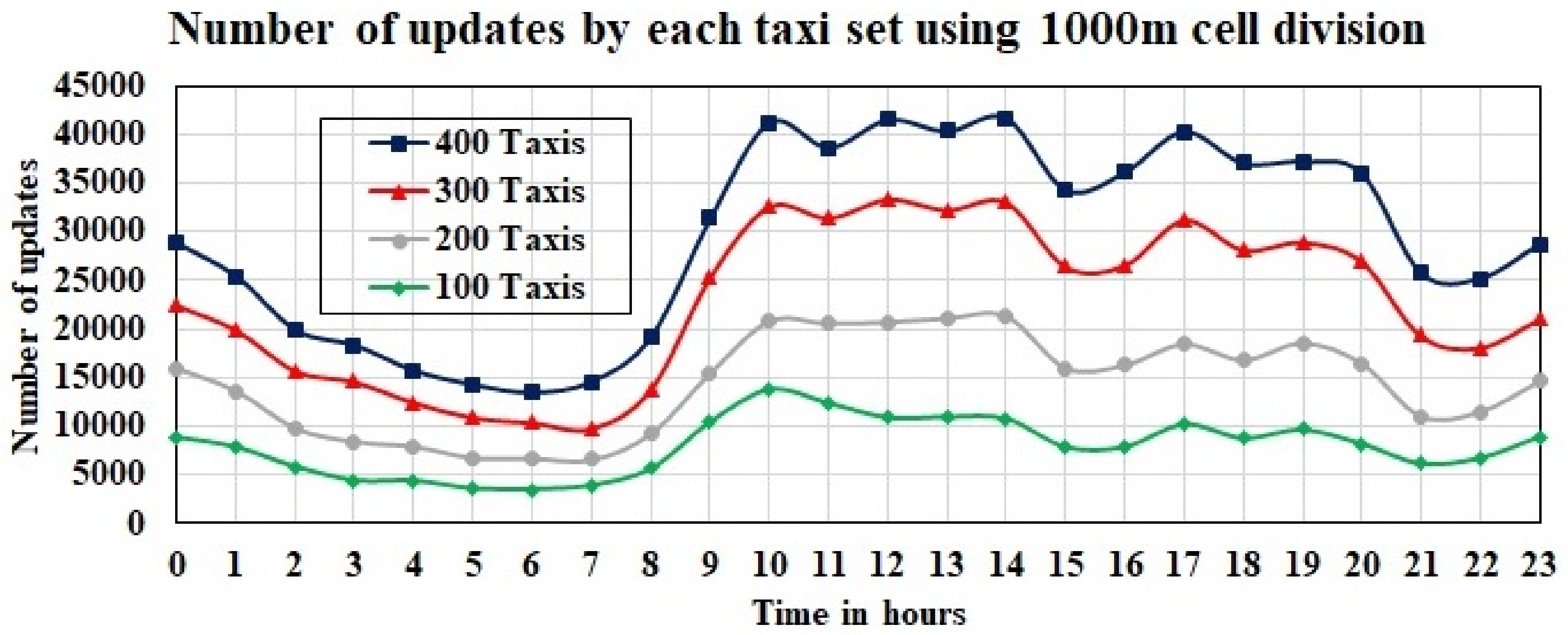
The estimates of this analysis can be matched with the requirements of different applications that can be supported by the proposed vehicular network. For example, the amount of data generated from the smart sensors by knowing the requirements of different smart city data applications, and the delay-tolerant intervals, which is helpful to decide the radio technology that can support. Data transmission capacity is a key component to measure the application requirements of a smart city that can be supported by the proposed vehicular communication. For this purpose, we can associate the total time a taxicab remains in the wireless range of the grid with the time to travel between source and destination grids. For that purpose, we need the number of updates recorded by each vehicle in each grid and the total time a vehicle remains inside each grid.

We got the location updates of taxis in each grid after the formation of grids by our grid clustering algorithm over the time intervals of 24 h. When we increase the radio range of technology, we get a higher number of vehicle contacts inside the grid. In our analysis, the biggest cluster obtained has 12,260 updates by taxicabs in a day with a grid size of 1000 m${}^2$. When we decrease the grid size, we get a smaller number of updates. The grid size of 500 m${}^2$ receives 9483 and that of 250 m${}^2$ receives 9415, and the grid size of 100 m${}^2$ receives 9248 updates, respectively.

Figure 8 represents the total time in seconds that all vehicles remain inside a grid in the time interval of 24 h. This sum compares the absolute time that these taxicabs can use to offload information to the vehicular network in 24 h. Each group of vertical bars relates to a different radio range varying from 100 m${}^2$ to 1000 m${}^2$. A rectangular cluster is created by all taxicabs that update their position inside a grid. In this manner, if a taxicab remains in a cluster for a longer time, it implies that it appears more than once in this grid. Since these clusters are formulated by the number of updates reported by taxicabs, so there is an immediate connection to staying time. Moreover, there is an association with the number of taxicabs inside a grid because when a taxicab has a limited number of updates each day, a grid cluster receives more updates from the most active area of the city.

We can employ the multiplying factor to calculate the aggregated data volume that can be collected in an interval of 24 h, the data rate related to each radio technology, and that all taxicabs remain in the wireless coverage area of the grid cluster introduced in Figure 8. However, it is crucial to determine this multiplying factor accurately because there are many other variables involved to be considered for actual calculations. We can find a few reflections on the throughput of data communication in vehicular networks as follows. In [53], authors define the data rates of IEEE 802.11p at 9, 18, 36, 48, 54 Mbps by using different modulation techniques with a wireless range up to 1000 m${}^2$ outdoor and frequency band of 20 MHz bandwidth. In [54], authors calculated the data rates of IEEE 802.11n 600 Mbps with frequency range 20 MHz to 40 MHz at modulation MIMO-OFDM where wireless ranges are up to 250 m outdoor. In [55], authors define the data rate of IEEE 802.11ay up to 100 Gbps. In [5], authors define the data rate as 20 Gbps in an outdoor wireless range of 100 m${}^2$ with frequency band 8000 MHz at OFDM modulation. In IEEE 802.16, WiMax provides mobile and fixed internet access. It can provide data rates up to 1 Gbps with a frequency band of 2 GHz and 11 GHz [56]. This brief survey on literature shows that there is a great capability of data transfer among vehicles and fixed infrastructures. Each of these studies uses different conditions and equipment, which create outcomes in a distinctive test-bed. It is difficult to fix the multiplying factor for throughput of data in the vehicle-to-infrastructure case because of different conditions and equipment. Hence, supported by the literature, we select IEEE 802.11p for 1000 m${}^2$ cluster for smart devices to the vehicle and the vehicle to the RSUs, IEEE 802.16 for the 500 m${}^2$ cluster, IEEE 802.11n for 250 m${}^2$ cluster, and IEEE 802.11ay for 100 m${}^2$ cluster. In this case, the multiplying factors are, 54 Mbps for IEEE 802.11p, 1Gbps for IEEE 802.16, 600 Mbps for IEEE 802.11n and 20 Gbps for IEEE 802.11ay, as seen in [5,53,54,55,56].

We have shown the selected sell sizes and supporting technologies with their multiplying factors in

Table 3. Capacity of data offloading in SC architecture with different clusters and data rates of selected wireless technologies.

Cell Size	Technology Assumed	Data Rates in Mbps	Data Transfer Capacity in PB
			400 Taxi	300 Taxi	200 Taxi	100 Taxi
1000 m	IEEE 802.11p	54	0.133	0.103	0.065	0.036
500 m	IEEE 802.16	1000	2.463	1.901	1.204	0.670
250 m	IEEE 802.11n	600	1.477	1.141	0.722	0.402
100 m	IEEE 802.11ay	20,480	51.135	38.966	24.661	13.733

. We can get the potential of the proposed network against each selected set of vehicles by applying the multiplying factor with the total stay time of vehicles in the corresponding grids. For example, in a grid size of 1000 m${}^2$ and throughput of 54 Mbps, IEEE 802.11p can reach up to 0.133 PB in case of a bigger set of taxicabs. As the size of the grid grows, the number of updates by vehicles in that grid also grows, which implies the greater stay time in that grid as shown in Figure 8. On the other hand, the table shows that the throughput of selected technologies increases in the case of smaller grid sizes, where taxicabs have less stay time. For example, the capacity with IEEE 802.16 reaches up to 2.463 PB. However, it is the most expensive technology because it requires a huge infrastructure to implement. IEEE 802.11n provides 1.477 PB capacity with 250 m${}^2$ grid size. IEEE 802.11ay can reach up to 13.733 PB at the smallest grid size of 100 m${}^2$ and with the smallest set of taxicabs. Our results show that the capacity of the network does not merely depend upon the vehicles’ stay time in a cluster, but the selected communication technology does matter as well.

4.6. Hourly Updates of Different Clusters

Figure 9 explains the stay time of all selected taxis in the area of 1000 m per hour throughout the day. Please note that the time of day affects system capacity. During peak hours, traffic congestion increases significantly. So, there are more taxis to meet people’s needs, from their homes to their workplaces. However, the less crowded time from 9 p.m. to 9 a.m. leads to reduced capacity. On the other hand, Figure 10 shows an interesting factor, which gives hourly updates of the largest taxi group throughout the day, in the top 10 clusters of each size. It shows that the number of taxi updates is highest between 3 a.m. and 8 a.m. During this time period, taxis are moving slowly, they are still staying in the most popular areas of the city, and the job ratio is still high. This time interval is more suitable for transmitting data from the taxi to the data centers. This fact can help us to deploy the RSU network for the data center and the right time for data offloading in the data center.

4.7. Data Offloading a Service Scenario

We suggest a new software update for smart devices that may be available by the service providers at some given time. We can evaluate the data offloading performance of our proposed network when the service provider can forward these updates to smart devices. One of the cases is, the service provider will send this data directly to devices. For this purpose, each device should have a sim card to connect it with the cellular network or it should be directly attached to the internet. This case requires a high cost for infrastructure deployment. In our proposed solutions, the service provider will forward this update to the CC server. From the CC server, data will be forwarded to smart devices by using our proposed network.

We consider the following two cases for the evaluation of our proposed network. First, smart vehicles can directly receive this software update from the CC server through the internet since they are connected to the internet. The CC server selects a set of vehicles and forwards this update to those vehicles. After getting this data, vehicles start the diffusion process and transmit this data to smart devices whenever they are in their wireless range. In this diffusion process, vehicles should be helpful as they use their resources in terms of internet connection if this is not impact their trajectory.

On the other hand, whenever the CC server receives the software update, it will forward this data to RSUs. Now, vehicles will pick the data whenever they are in the wireless range of these RSUs and start the diffusion process. After collecting data from RSUs, the vehicles transfer data to smart devices whenever they are in their wireless range. In this case, we apply the greedy Algorithm 5 on Beijing city traces to identify the most popular location of the selected area as shown in Figure 11. The cluster size for this evaluation is considered equal to 1000 m${}^2$ and the number of taxi-cabs as 400. We consider the case of 1000 m${}^2$ grids and identify 36 locations. We assumed that RSUs are installed at these locations and are directly connected to the CC server by the internet. In this case, there is no need to share the internet connections of smart vehicles. This process will be slow compared to direct communication because a vehicle will first visit in any of RSU installed grid clusters, then it will start the diffusion process.

We do not consider any particular propagation model and pairing delay in both of the cases because our proposed network is independent of any wireless technology. Figure 12 shows the delay is higher than when there is direct communication. As the delay-tolerant interval increases, the coverage in both cases increases, which is around 98% in direct communication and 96% otherwise when we use the RSUs. When we have a higher delay-tolerant interval, then the latter case under RSUs provides good coverage and saves the cost of internet connections to smart vehicles.

5. Limitations

This work provides components for the effective design of data dissemination through delay-tolerant vehicle networks in smart cities. The main purpose of this research is to identify the singularity of the network and estimate the network dynamics. Through the given analysis, we anticipate the formation of specific user needs, determine the prospects for realizing a suitable network, and help find the type of transmission technology that should be applied to achieve the desired goals. It can also find the network coverage of different wireless technologies coverage areas in smart cities. From a practical point of view, it is very interesting to determine the data transmission capabilities of each technology through the actual data transmission between the vehicle and the grid, and between the vehicles. With such research results, it is recommended to replace the value of the data rate “multiplication factor” in our analysis model with empirical results.

This research is based on the analysis of vehicle big data in smart city scenarios. However, the actual data packet exchange between the vehicle and the cluster is not considered. This means that we do not consider aspects such as the physical layer and the connection time when the vehicle is within the wireless range of the device. In our research, these parameters are finally considered by assuming a “multiplier”, which can simulate the recommended capacity of the wireless link and replace it with a constant value determined in the literature that takes into account the peculiarities of the physical layer. In addition, this study generally calculates the capacity of data transmission, so it does not consider the configuration of any transmission protocol for a specific wireless system or application. However, the required protocol can be determined by seeking to minimize the latency of a given data requirement and create competitive results for the specific application along with the lines of this model.

6. Conclusions

In this paper, we propose an alternate network in a smart city that does not require the deployment of expensive infrastructure to collect delay-tolerant data. We have studied the data dissemination potential of the vehicular network from the aspects of network coverage and capacity. We used the microscopic movement of the taxi and its GPS position in Beijing to evaluate our proposed SC network architecture. We apply the region partitioning algorithm to large spatio-temporal data to reduce the complexity. We evaluated the density of vehicles in a given area, which was further used to find potential locations for data offloading. Our results show that a relatively small part of the taxi fleets operating in a large area (25 × 25 km${}^2$) in Beijing can reach more than 90% of coverage within 24 h when the grid size is greater than 500 m${}^2$. Our proposed network can be used to collect a significant amount of data that can be offloaded to vehicles. Using the IEEE 802.11n standard, the network can collect more than 1.4 PB of data per day. We found that the our network is suitable for delay-tolerant data delivery applications because it can further reduce network load by sharing the burden of congested network. The hourly update analysis of taxi trajectory data can help designers find the most suitable unit for RSU deployment. Data dissemination case studies show that as long as there is a loose time demand, the proposed network can perform well. In future work, the proposed model can be used to analyze and find the optimal vehicle and RSU to transmit data/code, minimize the data transmission time, and enhance the data coverage using the historical trajectory information of the vehicle. In addition, it would be also very interesting to realize the proposed network model by considering the characteristics of the communication protocol in the wireless sensor network.

References

1. Cheng, N.; Lu, N.; Zhang, N.; Shen, X.S.; Mark, J.W. Vehicular WiFi offloading: Challenges and solutions. Veh. Commun. 2014, 1, 13–21. [Google Scholar] [CrossRef] [Green Version]
2. Luan, T.H.; Shen, X.; Bai, F.; Sun, L. Feel bored? Join verse! Engineering vehicular proximity social networks. IEEE Trans. Veh. Technol. 2014, 64, 1120–1131. [Google Scholar] [CrossRef]
3. Rebecchi, F.; De Amorim, M.D.; Conan, V.; Passarella, A.; Bruno, R.; Conti, M. Data offloading techniques in cellular networks: A survey. IEEE Commun. Surv. Tutor. 2014, 17, 580–603. [Google Scholar] [CrossRef] [Green Version]
4. Naseer, S.; Liu, W.; Sarkar, N.I.; Chong, P.H.J.; Lai, E.; Prasad, R.V. A sustainable vehicular based energy efficient data dissemination approach. In Proceedings of the 27th International Telecommunication Networks and Applications Conference (ITNAC), Melbourne, Australia, 22–24 November 2017; pp. 1–8. [Google Scholar]
5. Naseer, S.; Liu, W.; Sarkar, N.I. Energy-Efficient Massive Data Dissemination through Vehicle Mobility in Smart Cities. Sensors 2019, 19, 4735. [Google Scholar] [CrossRef] [PubMed] [Green Version]
6. Naseer, S.; Liu, W.; Sarkar, N.I.; Chong, P.H.J.; Lai, E.; Ma, M.; Prasad, R.V.; Danh, T.C.; Chiaraviglio, L.; Qadir, J.; et al. A sustainable marriage of telcos and transp in the era of big data: Are we ready? In International Conference on Smart Grid Inspired Future Technologies; Springer: Cham, Switzerland, 2018. [Google Scholar]
7. Zhang, Z. Routing in intermittently connected mobile ad hoc networks and delay tolerant networks: Overview and challenges. IEEE Commun. Surv. Tutor. 2006, 8, 24–37. [Google Scholar] [CrossRef] [Green Version]
8. Shah, R.C.; Roy, S.; Jain, S.; Brunette, W. Data mules: Modeling and analysis of a three-tier architecture for sparse sensor networks. Ad Hoc Netw. 2003, 1, 215–233. [Google Scholar] [CrossRef]
9. Anastasi, G.; Conti, M.; Di Francesco, M. Data collection in sensor networks with data mules: An integrated simulation analysis. In Proceedings of the 2008 IEEE Symposium on Computers and Communications, Marrakech, Morocco, 6–9 July 2008; pp. 1096–1102. [Google Scholar]
10. Anastasi, G.; Conti, M.; Monaldi, E.; Passarella, A. An adaptive data-transfer protocol for sensor networks with data mules. In Proceedings of the 2007 IEEE International Symposium on a World of Wireless, Mobile and Multimedia Networks, Espoo, Finland, 18–21 June 2007; pp. 1–8. [Google Scholar]
11. Zhao, W.; Ammar, M.; Zegura, E. A message ferrying approach for data delivery in sparse mobile ad hoc networks. In Proceedings of the 5th ACM International Symposium on Mobile ad Hoc Networking and Computing, Tokyo, Japan, 24–26 May 2004; pp. 187–198. [Google Scholar]
12. Kansal, A.; Rahimi, M.; Estrin, D.; Kaiser, W.J.; Pottie, G.J.; Srivastava, M.B. Controlled mobility for sustainable wireless sensor networks. In Proceedings of the First Annual IEEE Communications Society Conference on Sensor and Ad Hoc Communications and Networks (IEEE SECON 2004), Santa Clara, CA, USA, 4–7 October 2004; pp. 1–6. [Google Scholar]
13. Felegyhazi, M.; Hubaux, J.P.; Buttyan, L. Nash equilibria of packet forwarding strategies in wireless ad hoc networks. IEEE Trans. Mob. Comput. 2006, 5, 463–476. [Google Scholar] [CrossRef]
14. Sugihara, R.; Gupta, R.K. Path planning of data mules in sensor networks. ACM Trans. Sens. Netw. (TOSN) 2011, 8, 1–27. [Google Scholar] [CrossRef]
15. Naseer, S.; Liu, W.; Sarkar, N.I.; Chong, P.H.J.; Lai, E.; Ma, M.; Prasad, R.V.; Danh, T.C.; Chiaraviglio, L.; Qadir, J.; et al. A sustainable marriage of telcos and transp in the era of big data: Are we ready? In Smart Grid and Innovative Frontiers in Telecommunications; Springer: Cham, Switzerland, 2018; pp. 210–219. [Google Scholar] [CrossRef]
16. Munjal, R.; Liu, W.; Li, X.J.; Gutierrez, J.; Furdek, M. Sustainable massive data dissemination by using software defined connectivity approach. In Proceedings of the 27th International Telecommunication Networks and Applications Conference (ITNAC), Melbourne, Australia, 22–24 November 2017; pp. 1–6. [Google Scholar]
17. Munjal, R.; Liu, W.; Li, X.J.; Gutierrez, J.; Chong, P.H.J. Telco asks transp: Can you give me a ride in the era of big data? In Proceedings of the IEEE Conference on Computer Communications Workshops (INFOCOM WKSHPS), Atlanta, GA, USA, 1–4 May 2017; pp. 766–771. [Google Scholar]
18. Munjal, R.; Liu, W.; Li, X.J.; Gutierrez, J. Big Data Offloading using Smart Public Vehicles with Software Defined Connectivity. In Proceedings of the IEEE Intelligent Transportation Systems Conference (ITSC), Auckland, New Zealand, 27–30 October 2019; pp. 3361–3366. [Google Scholar]
19. Munjal, R.; Liu, W.; Li, X.J.; Gutierrez, J.; Furdek, M. Sustainable Crowdsensing Data Dissemination Using Public Vehicles. In Crowd Assisted Networking and Computing; CRC Press: Boca Raton, FL, USA, 2018; pp. 77–110. [Google Scholar]
20. Gerla, M.; Lee, E.K.; Pau, G.; Lee, U. Internet of vehicles: From intelligent grid to autonomous cars and vehicular clouds. In Proceedings of the 2014 IEEE World Forum on Internet of Things (WF-IoT), Seoul, Korea, 6–8 March 2014; pp. 241–246. [Google Scholar]
21. Rebai, M.; Khoukhi, L.; Snoussi, H.; Hnaien, F. Optimal placement in hybrid VANETs-sensors networks. In Proceedings of the 2012 Wireless Advanced (WiAd), London, UK, 25–27 June 2012; pp. 54–57. [Google Scholar]
22. Qin, H.; Li, Z.; Wang, Y.; Lu, X.; Zhang, W.; Wang, G. An integrated network of roadside sensors and vehicles for driving safety: Concept, design and experiments. In Proceedings of the 2010 IEEE International Conference on Pervasive Computing and Communications (PerCom), Mannheim, Germany, 29 March–2 April 2010; pp. 79–87. [Google Scholar]
23. Campolo, C.; Molinaro, A.; Scopigno, R. From today’s VANETs to tomorrow’s plan-ning and the bets for the day after. Veh. Commun. 2015, 2, 158–171. [Google Scholar]
24. Araniti, G.; Campolo, C.; Condoluci, M.; Iera, A.; Molinaro, A. LTE for vehicular networking: A survey. IEEE Commun. Mag. 2013, 51, 148–157. [Google Scholar] [CrossRef]
25. Baron, B.; Campista, M.; Spathis, P.; Costa, L.H.M.; de Amorim, M.D.; Duarte, O.C.M.; Pujolle, G.; Viniotis, Y. Virtualizing vehicular node resources: Feasibility study of virtual machine migration. Veh. Commun. 2016, 4, 39–46. [Google Scholar] [CrossRef] [Green Version]
26. Piro, G.; Orsino, A.; Campolo, C.; Araniti, G.; Boggia, G.; Molinaro, A. D2D in LTE vehicular networking: System model and upper bound performance. In Proceedings of the 2015 7th International Congress on Ultra Modern Telecommunications and Control Systems and Workshops (ICUMT), Brno, Czech Republic, 6–8 October 2015; pp. 281–286. [Google Scholar]
27. Li, H.; Wang, B.; Song, Y.; Ramamritham, K. VeShare: A D2D infrastructure for real-time social-enabled vehicle networks. IEEE Wirel. Commun. 2016, 23, 96–102. [Google Scholar] [CrossRef]
28. Gorcitz, R.A.; Jarma, Y.; Spathis, P.; de Amorim, M.D.; Wakikawa, R.; Whitbeck, J.; Conan, V.; Fdida, S. Vehicular carriers for big data transfers (poster). In Proceedings of the 2012 IEEE Vehicular Networking Conference (VNC), Seoul, Korea, 14–16 November 2012; pp. 109–114. [Google Scholar]
29. Mitton, N.; Rivano, H. On the use of city bikes to make the city even smarter. In Proceedings of the 2014 International Conference on Smart Computing Workshops, Hong Kong, China, 5 November 2014; pp. 3–8. [Google Scholar]
30. dos Santos, A.D.J.; Costa, L.H.M.; de Lima Braga, M.; Velloso, P.B.; Ghamri-Doudane, Y. Characterization of a delay and disruption tolerant network in the Amazon basin. Veh. Commun. 2016, 5, 35–43. [Google Scholar] [CrossRef]
31. Bai, F.; Sadagopan, N.; Helmy, A. The IMPORTANT framework for analyzing the Impact of Mobility on Performance Of RouTing protocols for Adhoc NeTworks. Ad hoc Netw. 2003, 1, 383–403. [Google Scholar] [CrossRef]
32. Härri, J.; Filali, F.; Bonnet, C.; Fiore, M. VanetMobiSim: Generating realistic mobility patterns for VANETs. In Proceedings of the 3rd International Workshop on Vehicular Ad Hoc Networks, Los Angeles, CA, USA, 29 September 2006; pp. 96–97. [Google Scholar]
33. Smith, L.; Beckman, R.; Baggerly, K. TRANSIMS: Transportation Analysis and Simulation System (No. LA-UR-95-1641); Los Alamos National Lab.: Los Alamos, NM, USA, 1995. [Google Scholar]
34. Krajzewicz, D.; Erdmann, J.; Behrisch, M.; Bieker, L. Recent development and applications of SUMO-Simulation of Urban MObility. Int. J. Adv. Syst. Meas. 2012, 5, 128–138. [Google Scholar]
35. Pan, G.; Qi, G.; Zhang, W.; Li, S.; Wu, Z.; Yang, L.T. Trace analysis and mining for smart cities: Issues, methods, and applications. IEEE Commun. Mag. 2013, 51, 120–126. [Google Scholar] [CrossRef]
36. Bai, F.; Krishnamachari, B. Spatio-temporal variations of vehicle traffic in VANETs: Facts and implications. In Proceedings of the Sixth ACM International Workshop on Vehicular Internetworking, Beijing, China, 15–16 September 2009; pp. 43–52. [Google Scholar]
37. Uppoor, S.; Trullols-Cruces, O.; Fiore, M.; Barcelo-Ordinas, J.M. Generation and analysis of a large-scale urban vehicular mobility dataset. IEEE Trans. Mob. Comput. 2013, 13, 1061–1075. [Google Scholar] [CrossRef] [Green Version]
38. Chen, Y.; Xu, M.; Gu, Y.; Li, P.; Cheng, X. Understanding topology evolving of VANETs from taxi traces. Adv. Sci. Technol. Lett. 2013, 42, 13–17. [Google Scholar]
39. Liu, B.; Khorashadi, B.; Ghosal, D.; Chuah, C.N.; Zhang, H.M. Analysis of the information storage capability of VANET for highway and city traffic. Transp. Res. Part C Emerg. Technol. 2012, 23, 68–84. [Google Scholar] [CrossRef]
40. Piorkowski, M.; Sarafijanovic-Djukic, N.; Grossglauser, M. A parsimonious model of mobile partitioned networks with clustering. In Proceedings of the 2009 First International Communication Systems and Networks and Workshops, Bangalore, India, 5–10 January 2009; pp. 1–10. [Google Scholar]
41. Mougenot, D.; Liu, J. Single-Sensor HD-3D in China: Case Studies from MEMS-Based Accelerometers. Available online: http://www.sercel.com/products/Lists/ProductPublication/Single-sensor%20HD-3D%20in%20China_case%20studies%20from%20MEMS-based%20accelerometers_dec2012.pdf (accessed on 30 November 2020).
42. Liu, B.; Khorashadi, B.; Ghosal, D.; Chuah, C.N.; Zhang, M.H. Assessing the VANET’s local information storage capability under different traffic mobility. In Proceedings of the 2010 IEEE INFOCOM, San Diego, CA, USA, 14–19 March 2010; pp. 1–5. [Google Scholar]
43. Palma, V.; Vegni, A.M. On the Optimal Design of a Broadcast Data Dissemination System over VANET Providing V2V and V2I Communications “The Vision of Rome as a Smart City”. J. Telecommun. Inf. Technol. 2013, 1, 41–48. [Google Scholar]
44. Aslam, J.; Lim, S.; Pan, X.; Rus, D. City-scale traffic estimation from a roving sensor network. In Proceedings of the 10th ACM Conference on Embedded Network Sensor Systems, Toronto, ON, Canada, 6–9 November 2012; pp. 141–154. [Google Scholar]
45. Cho, Y.S.; Kim, J.; Yang, W.Y.; Kang, C.G. MIMO-OFDM Wireless Communications with MATLAB; John Wiley & Sons: Hoboken, NJ, USA, 2010. [Google Scholar]
46. Wang, W.; Yang, J.; Muntz, R. STING: A statistical information grid approach to spatial data mining. VLDB 1997, 97, 186–195. [Google Scholar]
47. Zheng, Y. T-Drive Trajectory Data Sample. Available online: https://www.microsoft.com/en-us/research/publication/t-drive-trajectory-data-sample/ (accessed on 27 December 2020).
48. Nils, S. Plot Colored by Kernel Density Estimate. Available online: https://www.mathworks.com/matlabcentral/fileexchange/65728-scatter-plot-colored-by-kernel-density-estimate (accessed on 27 December 2020).
49. Guilford, G. A Big Reason Beijing Is Polluted: The Average Car Goes 7.5 Miles per Hour. 2 July 2019. Available online: https://qz.com/163178/a-big-reason-beijing-is-polluted-the-average-car-goes-7-5-miles-per-hour/ (accessed on 31 December 2020).
50. Yuan, J.; Zheng, Y.; Xie, X.; Sun, G. Driving with knowledge from the physical world. In Proceedings of the 17th ACM SIGKDD International Conference on Knowledge Discovery and Data Mining, San Diego, CA, USA, 21–24 August 2011; pp. 316–324. [Google Scholar]
51. Yuan, J.; Zheng, Y.; Zhang, C.; Xie, W.; Xie, X.; Sun, G.; Huang, Y. T-drive: Driving directions based on taxi trajectories. In Proceedings of the 18th SIGSPATIAL International Conference on Advances in Geographic Information Systems, San Jose, CA, USA, 2–5 November 2010; pp. 99–108. [Google Scholar]
52. Atlas of Urban Expansion, Region: East Asia and the Pacific, Beijing, China. Available online: http://www.atlasofurbanexpansion.org/cities/view/Beijing_Beijing (accessed on 15 July 2020).
53. Abdelgader, A.M.; Lenan, W. The physical layer of the IEEE 802.11 p WAVE communication standard: The specifications and challenges. In Proceedings of the World Congress on Engineering and Computer Science, San Francisco, CA, USA, 22–24 October 2014; Volume 2, pp. 22–24. [Google Scholar]
54. Vanhatupa, T. Wi-Fi Capacity Analysis for 802.11 ac and 802.11 n: Theory & Practice; Ekahau Inc.: Reston, VA, USA, 2013. [Google Scholar]
55. Ghasempour, Y.; da Silva, C.R.; Cordeiro, C.; Knightly, E.W. IEEE 802.11 ay: Next-generation 60 GHz communication for 100 Gb/s Wi-Fi. IEEE Commun. Mag. 2017, 55, 186–192. [Google Scholar] [CrossRef]
56. Elias, S.J.; Warip, M.N.B.M.; Ahmad, R.B.; Halim, A.H.A. A comparative study of IEEE 802.11 standards for non-safety applications on vehicular ad hoc networks: A congestion control perspective. In Proceedings of the World Congress on Engineering and Computer Science, San Francisco, CA, USA, 22–24 October 2014; Volume 2, p. 33. [Google Scholar]
Figure 1. Smart city scenario for data dissemination [5].
Sustainability 13 10907 g001
Figure 2. Effective distance.
Sustainability 13 10907 g002
Figure 3. Heat map of vehicle density in Beijing under the selected area of 25 × 25 km 2 by visualization of T-Drive traces data set.
Sustainability 13 10907 g003
Figure 4. Heat table of vehicle density in each cluster with size 1000 × 1000 m 2 .
Sustainability 13 10907 g004
Figure 5. Percentage of grid coverage in terms of weekday, weekend, and average week.
Sustainability 13 10907 g005
Figure 6. Percentage of grid coverage with different cell sizes.
Sustainability 13 10907 g006
Figure 7. Percentage of grid overage with different subsets of taxicabs.
Sustainability 13 10907 g007
Figure 8. Stay time inside the cluster of different sizes with each taxicab subset.
Sustainability 13 10907 g008
Figure 9. Number of updates by each taxi set using 1000 m 2 cell division.
Sustainability 13 10907 g009
Figure 10. Hourly updates in top hundred cells of each category.
Sustainability 13 10907 g010
Figure 11. Location of roadside units.
Sustainability 13 10907 g011
Figure 12. Percentage of clusters reached during data diffusion process.
Sustainability 13 10907 g012