Article

Relating Land Use/Cover and Landscape Pattern to the Water Quality under the Simulation of SWAT in a Reservoir Basin, Southeast China

1
Institute of Land Science and Property, School of Public Affairs, Zhejiang University, Hangzhou 310058, China
2
College of Materials and Environmental Engineering, Hangzhou Dianzi University, Hangzhou 310018, China
*
Author to whom correspondence should be addressed.
Sustainability 2021, 13(19), 11067; https://doi.org/10.3390/su131911067
Submission received: 25 July 2021 / Revised: 9 September 2021 / Accepted: 29 September 2021 / Published: 7 October 2021

Abstract

:
Understanding the relationship between land use/cover pattern and water quality could provide guidelines for non-point source pollution and facilitate sustainable development. The previous studies mainly relate the land use/cover of the entire region to the water quality at the monitoring sites, but the water quality at monitoring sites did not totally reflect the water environment of the entire basin. In this study, the land use/cover was monitored on Google Earth Engine in Tang-Pu Reservoir basin, China. In order to reflect the water quality of the whole study area, the spatial distribution of the determinants for water quality there, i.e., the total nitrogen and total phosphorus (TN&TP), were simulated by the Soil and Water Assessment Tool (SWAT). The redundancy analysis explored the correlations between land use/cover pattern and simulated TN&TP. The results showed that: (1) From 2009 to 2019, forest was the dominant land cover, and there was little land use/cover change. The landscape fragmentation increased, and the connectivity decreased. (2) About 25% TP concentrations and nearly all the TN concentrations at the monitoring points did not reach drinking water standard, which means nitrogen and phosphorus pollution were the most serious problems. The highest output per unit TN&TP simulated by SWAT were 44.50 kg/hm2 and 9.51 kg/hm2 and occurred in areas with highly fragile landscape patterns. (3) TN&TP correlated positively with cultivated and construction land but negatively with forest. The correlation between forest and TN&TP summited at 500–700-m buffer and construction land at 100-m buffer. As the buffer size increased, the correlation between the cultivated land, and the TN weakened, while the correlation with the TP increased. TN&TP correlated positively with the Shannon’s Diversity Index and negatively with the Contagion Index. This study provides a new perspective for exporting the impact of land use/cover pattern on water quality.

1. Introduction

Maintaining clean water exerts a pivotal function on habitat protection, agricultural production, and public health. However, it is challenging, especially due to the non-point source (NPS) pollution [1,2,3,4]. NPS pollution is mainly composed of soil sediment particles, nitrogen and phosphorus, and other nutrients, pesticides, etc., which enter the water, soil, or atmospheric environment through surface runoff, soil erosion, farmland drainage, etc. [5]. The rapid spread of urbanization, severe soil erosion, and excessive application of pesticides and fertilizers all have significant contributions to the NPS pollution of the regional water environment—an important environmental problem that must be resolved urgently [6,7].
The influence of land use/cover type on water quality has been a concern since the 1970s [8]. Previous studies have shown that the deterioration of water quality is driven by improper land use/cover due to anthropogenic activities [9,10]. Inappropriate land use/cover has an impact on the hydrological process of the basin by causing changes in the properties of the underlying surface and soil composition [11,12]. It can affect the process of runoff generation in the basin, further affecting the migration and transformation of NPS pollutants, especially nitrogen and phosphorus [5,13]. Castillo et al. [9] and Rodrigues et al. [14] noted that land use/cover type can increase nutrient loading and reduce nutrient retention, resulting in the eutrophication and hypoxia of the ecosystem. Other studies have found that the artificial regulation of land use/cover can control NPS pollution, thereby effectively supporting ecological functions [15]. Generally, studies have mainly focused on the impact of land use/cover type on water chemistry at different temporal and spatial scales. Mello et al. [16] collected samples to evaluate the land use/cover effects on water quality using Pearson’s correlation and redundancy analysis (RDA). Their results indicated that forest cover played a significant role in keeping the water clean, whereas agriculture and urban areas led to water quality degradation and placed immense pressure on the ecosystem. Based on Bayesian Networks, Xu et al. [17] established 20 monitoring stations and studied the response of water quality to land use/cover. They found that controlling water contaminant sources at a less than 20-km radii around monitoring stations could improve water quality efficiently, with farmlands acting as a “source” in wet seasons and as a “sink” in dry seasons.
Land use/cover composition is generally related to water quality, and landscape configuration controlling various biogeochemical and physical processes of the basin may be a more sensitive predictor of water quality [18,19,20]. There are many studies revealing that landscape metrics were significantly associated with water quality. Ding et al. [21] established 56 sampling sites and chose nine water parameters to reflect the water quality. They developed empirical models relating landscape metrics to the water quality using multivariate statistical analyses. The results illustrated that clean water quality was linked to the lower largest patch index of constructed land in plain catchments, whereas it was linked to a lower value for the patch densities of farmland, grassland, and orchard mountain watershed. Based on spatial filter regression of Moran’s Eigenvector, Janardan et al. [22] revealed that different land use/cover metrics had different scale effects, and water quality displayed highly temporal variations. At present, many studies have established sampling sites to measure water quality parameters so as to explore the impact of land use/cover and landscape pattern on water quality. However, the water quality at several sampling sites does not necessarily reflect the water quality of the entire basin. Thus, to better evaluate the complex impacts of land use/cover type and landscape pattern on water quality, it is necessary to quantify the correlation between land use/cover pattern and the water quality of the entire basin.
The Soil and Water Assessment Tool (SWAT) is a continuous, long-term, physically based distributed model developed to assess the impacts of climate and land management on hydrological components, sediment loading, and pollution transport in basins [23]. It has a wide range of applications and can be used for NPS pollution analysis [24,25]. When there is a lack of data, the SWAT model can be established by applying model parameter transplantation parameter transfer [26,27]. Zeiger et al. [28] used SWAT to simulate land use/cover impacts on streamflow, sediment, and nutrient loading in a karst catchment. Sertel et al. [25] evaluated the impact of land cover/use changes on watershed responses and hydrological processes in a rapidly urbanizing mid-latitude water supply catchment by applying SWAT. At this stage, many studies have focused on setting up a SWAT model and simulating runoff, sediment, and nutrients by land use/cover data. In addition, the NPS pollution scenarios based on the change of land use/cover have been studied extensively [25,29,30]. Rarely, studies established a correlation between land use/cover and water quality simulated by SWAT model.
It is crucial to investigate the relationship between land use/cover pattern and water quality, as this is conducive to optimizing land use/cover patterns and improving water-based ecological environment [31,32]. Previous studies have mainly focused on measuring water quality indicators at sampling sites to reflect the regional water environment, but this does not represent the pollution in its entirety. This study used the SWAT model to simulate the NPS pollution of the entire basin of the Tang-Pu Reservoir to explore the influence of land use/cover and landscape pattern on water quality. As a major national reservoir in southeast China, the Tang-Pu Reservoir has played a critical role in supplying water to the local community for drinking and agricultural purposes [33]. The maintenance of good water quality in the basin of the Tang-Pu Reservoir is of great significance to the stability of the local society and the lives of residents. Thus, understanding the relationship between land use/cover patterns and water quality can inform water pollution control and land use/cover management and help the government to make accurate decisions in the protection of water resources in the Tang-Pu Reservoir basin and similar basins. The main objectives of this study were to: (1) monitor the land use/cover and landscape pattern, (2) characterize the water quality and simulate the NPS pollution of water quality in the Tang-Pu Reservoir basin, and (3) reflect the relationships between TN&TP and land use/cover types and landscape pattern.

2. Materials and Methods
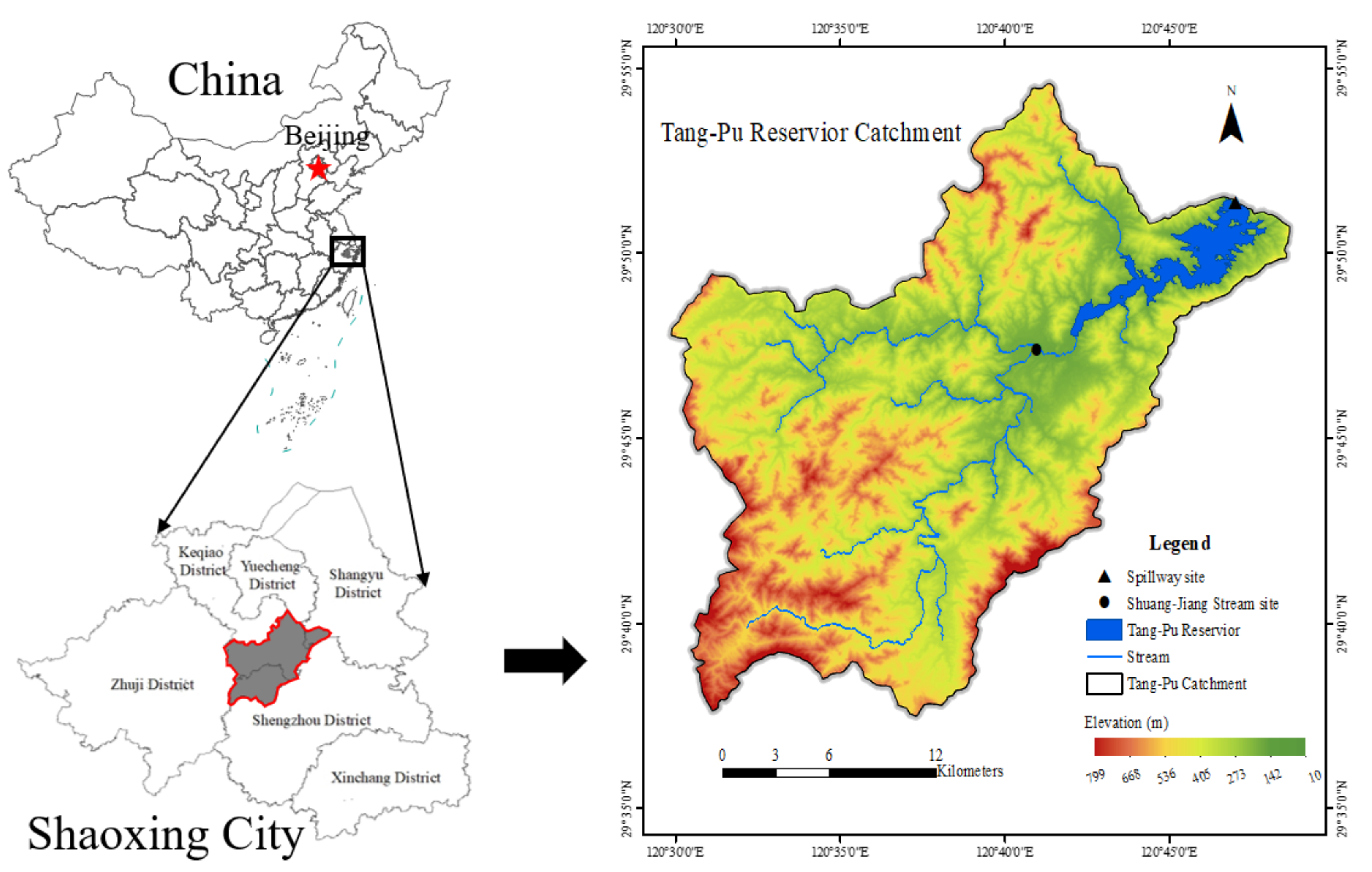
2.1. Study Region

The Tang-Pu Reservoir is located in the Shaoxing City, China (29°30′–29°57′ N, 120°24′–120°55′ E). It belongs to the Xiaoshun River Basin, a tributary of the Cao’e River, and encompasses an area of approximately 550 km2 with a total length of 70 km. The total storage capacity of the reservoir is 235 million m3, and the average water supply is 278.2 million m3. The Tang-Pu Reservoir supplies water to the local community of 5 million people for drinking and agricultural purposes. The topography in the basin is characterized by low mountain ranges and hills, and the terrain rises from northeast to southwest (Figure 1). The basin has a typical subtropical monsoonal climate, with an annual cycle of dry and wet seasons. The mean annual air temperature is 16.5 °C, and the mean annual amount of sunshine is 1903 h. The mean annual precipitation is 1564.4 mm, occurring during March, June, and September. In recent years, the average runoff of the basin is approximately 366 million m3, most of which is from precipitation. The soil type in this area is dominated by red soil and Acrisol. The predominant land use/cover type is forest, and the natural vegetation in the area is dominated by tree layers, most of which are masson pine. The main crops cultivated in the basin are cash crops, such as Torreya and tea, which are the main source of economy for the inhabitants of the area. The water environment of the river basin has been polluted by nitrogen and phosphorus recently, which has caused slight eutrophication of the reservoir environment, and the frequency of occurrence of eutrophication has increased [33].

2.2. Data

The data used in the study are shown in Table 1. Landsat 5 Thematic Mapper (TM) (30 m resolution; path 118 and row 39) images in October 2009 and Landsat 8 Operational Land Imager (OLI) (30 m resolution; path 118 and row 39) images in October 2019 were obtained from the Google Earth Engine (GEE) to detect the land use/cover and landscape patterns in the basin.
The Shaoxing Environmental Protection Section has established two sampling sites in the Tang-Pu Reservoir basin. One monitoring site, named Spillway, is located in the upstream with little anthropogenic activity, while the other monitoring site, named Shuang-Jiang Stream, is near the reservoir estuary (Figure 1). Water samples were collected once a month during 2017–2019. Six water quality parameters, including water temperature (TEM), pH, dissolved oxygen (DO), electrical conductivity (EC), TN, TP, and permanganate index (COD Mn), were analyzed according to the environmental quality standards for surface water (Chinese State Environmental Protection Bureau 2002). TEM (°C), and pH and EC (μs·cm−1) were measured on site using a portable conductivity meter (METTLER-SG3, Mettler Toledo, Columbus, OH, USA). DO (mg·L−1) was measured on site using a portable oxygen meter (YSI DO200, YSI Incorporated Company, Yellow Springs, OH, USA). TN (mg·L−1) was detected using the digestion-UV spectrophotometric method (UV2800, UNICO Company, South Brunswick, NJ, USA). COD Mn (mg·L−1) was determined by the potassium permanganate method. TP (mg·L−1) was measured using a spectrophotometer (UNICO2100, UNICO Company, South Brunswick, NJ, USA). The pretreatment and the determination of the parameters followed the national standard methods of examining water and wastewater, which were provided by the Ministry of Ecology and Environment, China.
The SWAT was applied in the Tang-Pu Reservoir to assess the impacts of land use/cover on hydrological components. The input data used in the SWAT model included a digital elevation model (DEM), soil data, digital land use/cover maps, meteorological data, hydrological data, and agricultural management information. The quality of the calculations performed is greatly influenced by the detail of the input data. We used a 12.5-m resolution DEM, from which the delineation of the sub-basins was determined as well as some topographic attributes (area, slope, slope length) and characteristics of their channel network [34]. The soil map was constructed from the Harmonized World Soil Database acquired from the Institute of Soil Science, Chinese Academy of Sciences. The soil input file defines the physical properties used by SWAT for all layers in the soil. There were many variables in the soil input file, such as soil type, depth, saturated hydraulic conductivity, and content of clay, silt, and sand. The local meteorological data, including daily precipitation, minimum and maximum temperature, average wind speed, average relative humidity, and solar radiation in the period from 2015 to 2019, were derived from Shaoxing meteorological stations. The hydrological data included the monthly flow data of the Shuang-Jiang Stream monitoring station from 2015 to 2019, and the water quality data included the total nitrogen and total phosphorus (TN&TP) data of the Shuang-Jiang Stream monitoring station from 2017 to 2019. These data were derived from the Shaoxing Ecological Environment Bureau. Agricultural management information was obtained from the local statistics yearbook.

2.3. Methods

2.3.1. Land Use/Cover Classification

Random forest classification has become an effective method in the remote sensing classification of machine learning [35]. It is an ensemble classifier that based on trees, and it can create new training sets by bagging techniques. When running the random forest method, random feature subspace enables faster tree building, and out-of-bag estimates evaluate the relative importance of each input feature [36].
Referring to the classification system of the Resource and Environment Science and Data Center, the land use/cover classes were categorized into five groups: (1) cultivated land, including paddy field and irrigated land; (2) garden land, including the orchard, tea garden, and other garden; (3) water, including rivers, reservoirs, and ponds; (4) forest, including wooded areas and mixed forest areas; and (5) constructed land, including residential land, road, and industrial land (Figure 1). The five land use/cover types were classified based on GEE using the random forest algorithm. About 105 samples were selected for each category, of which 80% of the samples were used for random classification, and 20% were used for accuracy validation.

2.3.2. Landscape Metrics for Landscape Pattern

Based on the classification map of land use/cover, landscape metrics were analyzed to characterize land use/cover patterns and investigate the effects of landscape configuration on water quality with the computer program FRAGSTATS 3.3. Because of the correlation among landscape metrics, a total of nine metrics were extracted to reduce the dependency and redundancy of the indices (Table 2), including Patch Density (PD), Largest Patch Index (LPI), Perimeter-Area Fractal Dimension (PAFRAC), Landscape Shape Index (LSI), Landscape Division Index (DIVISION), Splitting Index (SPLIT), Contagion Index (CONTAG), Shannon’s Diversity Index (SHDI), and Shannon’s Evenness Index (SHEI).

2.3.3. SWAT

SWAT was applied in the Tang-Pu Reservoir to assess the impacts of land use/cover on hydrological components [23]. In the SWAT model, a basin is divided into multiple sub-basins based on a DEM. The sub-basins are further divided into a series of uniform hydrological response units (HRUs) based on soil and land use/cover. After simulating the hydrological components, sediment yield, and nutrient cycles in each HRU, the results are aggregated for the sub-basins [37]. After adding all kinds of data, i.e., the soil chemical attribute data, local meteorological data, hydrological data, and agricultural management information, to the model, the SWAT model can be operated normally [38]. There are many parameters that have a great effect on the simulation results. To improve the reliability and applicability of the model, it is necessary to continuously modify the parameters of the model to verify the results [29,31]. The SWAT-CUP software provides a variety of uncertainty analysis algorithms. Among them, Sequential Uncertainty Fitting (SUFI2) was selected for sensitivity analysis, calibration, and verification of the model because of its high efficiency and accuracy according to previous studies [39]. In this paper, we regarded the sub-basin where the monitoring site of Shuang-Jiang Stream located as the area for calibration and verification. We selected January 2017 to December 2018 as the nutrient calibration period and January 2019 to December 2019 as the nutrient verification period to check their performances.
During the calibration and validation, the correlation coefficient (R2) and the Nash-Sutcliffe efficiency coefficient (NS) were selected to evaluate the applicability of the model and quantify the degree of fit between the measured value and simulation value. The validated model was applicable as the nutrient indices met the criteria recommended by Moriasi et al. [40], i.e., R2 > 0.0 and NS > 0.35 for phosphorus; R2 > 0.30 and NS > 0.35 for nitrogen. The mathematical formulas for the R2 and NS calculation are as follows:
R 2 = i = 1 n O i O ¯ P i P ¯ i = 1 n O i O ¯ 2 i = 1 n P i P ¯ 2 2
N S = 1 i = 1 n O i P i 2 i = 1 n O i O ¯ 2
where O i is the ith observed data, O ¯ is the mean value of observed data, P i is the ith simulation data, P ¯ is the mean value of simulation data, and the n is the total number of the observations.

2.3.4. Statistical analysis

RDA is an ordination method of the regression analysis combined with principal component analysis, which can reflect correlation between response variables and explanatory variables [41]. The explanatory variable that most influential for response can be found among the known environmental factors. RDA concentrates environmental factors in several ranking axes to indicate their impact on response variables, and the ranking axis is linear combination of the environmental factors [42]. RDA is widely used to determine the relationship between environmental factors and land use/cover in recent years. [21,41]. RDA allows us to examine the impact of multiple land use/cover variables on TN&TP simultaneously. There are two important results that can be output from RDA. One of which is ratio (%) of the total variance of TN&TP explained by ranking axes, and the other is the ordination diagrams, which definitely reveal the correlation between land use/cover pattern (environmental factor) and water quality parameters (species). In the species-environment ranking diagram, the direction and length of the arrow represent the correlation between species and environmental factors. The angle between the environmental factor and the species arrow indicate the correlation between the environmental factor and the species. If the angle between the two arrows is less than 90°, it means that there is a positive correlation between them; if it is greater than 90°, it indicates a negative correlation; and if it close to 90°, the correlation is weak. The length of the environmental factor arrow indicates the degree of its influence on the species data. The longer the arrow, the greater the explanation of the environmental factor to the response variable [43]. The RDAs were performed using the CANOCO 5.0 program (Microcomputer Power Company, Ithaca, New York, NY, USA).

3. Results

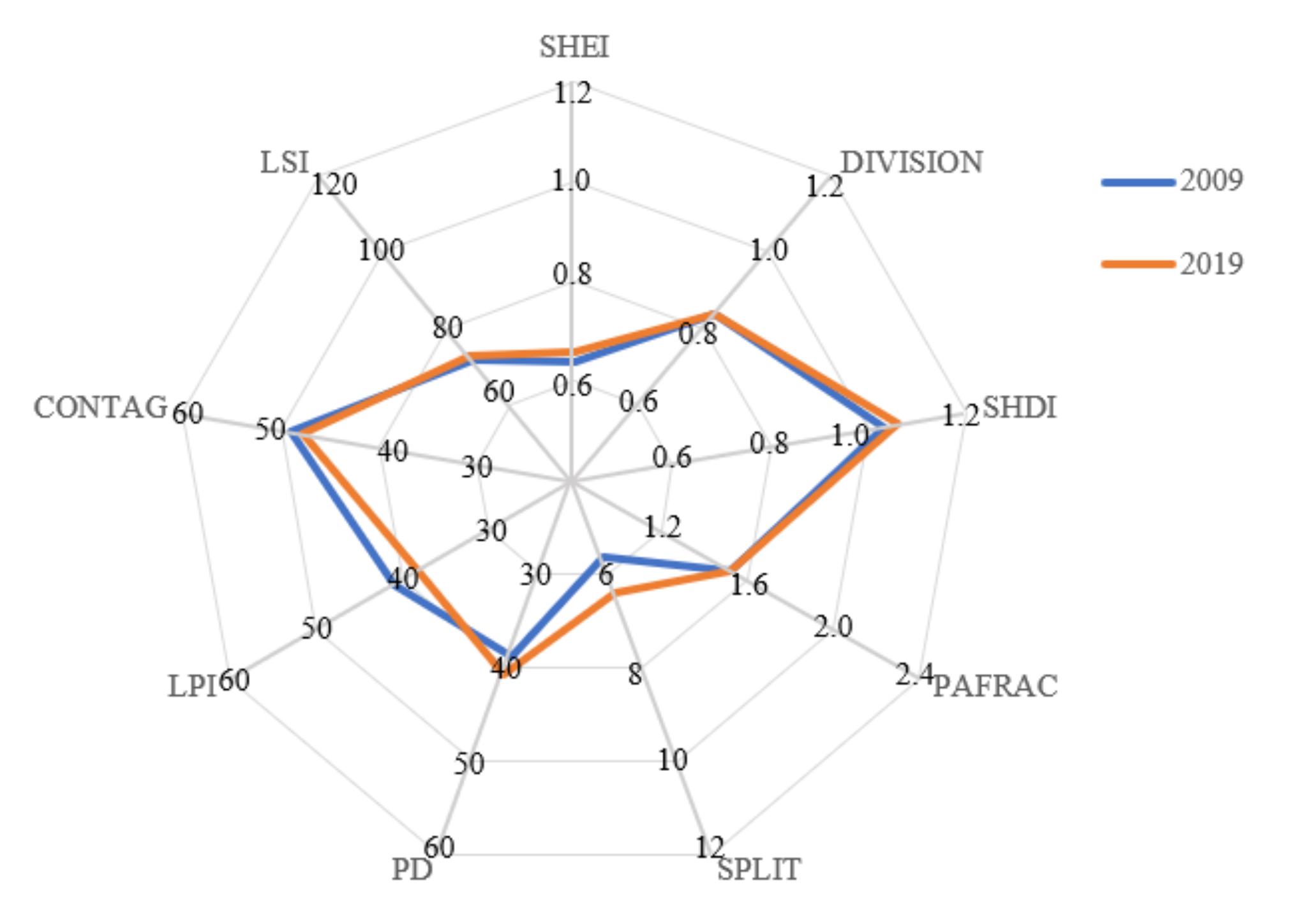
3.1. Land Use/Cover and Landscape Pattern Change Detection

The results of confusion matrix in 2009 and 2019 are shown in Table 3 and Table 4. They show that the overall accuracy of the land use/cover classification in the study area in 2009 and 2019 were 89% and 91%, respectively, and the Kappa coefficients land use/cover were 0.86 and 0.88, respectively, indicating that the classification accuracy met the requirements of land use/cover and cover classification.
The land use/cover classification map obtained by the random forest algorithm under the GEE platform is shown in Figure 2. Forest was the dominant land cover in the basin, and its percentage coverage accounted for more than 60%. Forest displayed a decreasing tendency during the years from 2009 to 2019 and was mainly converted to cultivated land and garden land. Garden land was also an important land use/cover in the basin, accounting for a percentage land cover of 16%. There was a slight increasing trend for the area of garden land from the period 2009 to 2019. Cultivated land was widely distributed across the basin, occupying > 11%. Cultivated land in the basin decreased between 2009 and 2019. Constructed land was mainly dispersed around the constructed land. Constructed land exhibited the most obvious change in the area, increasing by 3.53 km2 in the 10-year study period, and it occupied the area of surrounding cultivated land and gradually expanded outward. These changes emphasize that the Tang-Pu Reservoir is a mountainous area that is mainly covered by forest and is thus less affected by human disturbance. The increase in constructed land was mainly reflected in the increase in rural residential land and road land.
Figure 2. Land use/cover change in Tang-Pu Reservoir from 2009 to 2019. (a) Land use/cover in 2009; (b) land use/cover in 2009; (c) land use/cover transfer from 2009 to 2019. On the left is the area of land use/cover in 2009, and on the right is the area of land use/cover in 2019. The width of the flows represents the magnitude of the changes. Measured land use/cover pattern metrics changed at the landscape level, as shown in Figure 3. The landscape metrics of land use/cover differed significantly between 2009 and 2019. Among them, PD, LSI, SPLIT, SHDI, and SHEI increased, indicating that the landscape fragmentation in the area had increased, and the patch shape had become more complex. Meanwhile, LPI and CONTAG decreased, indicating that the dominance of the landscape and the connectivity of the landscape in the basin had decreased. PAFRAC and DIVISION remain basically unchanged.
Sustainability 13 11067 g002
Figure 3. Radar chart of each landscape pattern index in 2009 and 2019.
Sustainability 13 11067 g003

3.2. Water Quality of Tangpu Reservoir

3.2.1. Characteristics of Water Quality

The descriptive statistics of the original data for the seven water quality parameters are shown in Table 5. Each parameter can be identified the classification according to the environmental quality standards for surface water in China (GB3838-2002) [44]. Among them, class III is the minimum standard for human living drinking water, class IV is applicable to industrial water areas, and class V is applicable to agricultural water areas. DO varied greatly from 6.52 to 12.18 mg/L, with 78% of the samples exceeding water quality standards class I. The average concentration of COD Mn was 1.90 mg/L. More than half of the samples (65%) exceeded the class I water quality standard, with 32% exceeding class II water quality standards. The mean value of TP was 0.04 mg/L, with 7, 36, 32, and 22% of the samples exceeding water the quality standards class I, class II, class III, and class IV, respectively. In other words, 25% of the sampling sites for TP value did not meet class III, which is drinking water standard. Nitrogen pollution was the most serious pollution problem in the Tang-Pu Reservoir. The ratios for the mean values of TN compared to the class V standard of 2.0 mg N/L were 1.19. Nearly all the TN concentrations did not reach class III for the drinking water standard. Only about 35% of TN concentrations exceeded the class V water quality standard. The highest concentrations of TN were 2.88 times higher than the class V water quality standard. In summary, all of the water quality indicators in the Tang-Pu Reservoir basin had varying degrees of excessive pollution, especially TN&TP. Nitrogen and phosphorus pollution were the most serious pollution, causing eutrophication of the reservoir.
From the above study, it is clear that TN&TP were the most influencing factors for water quality in the study area, causing eutrophication of the reservoir. The following study focuses on nitrogen and phosphorus pollution. SWAT model simulated the output and their spatial distribution of TN&TP, and the relationship between land use/cover pattern and TN&TP in the basin was analyzed.

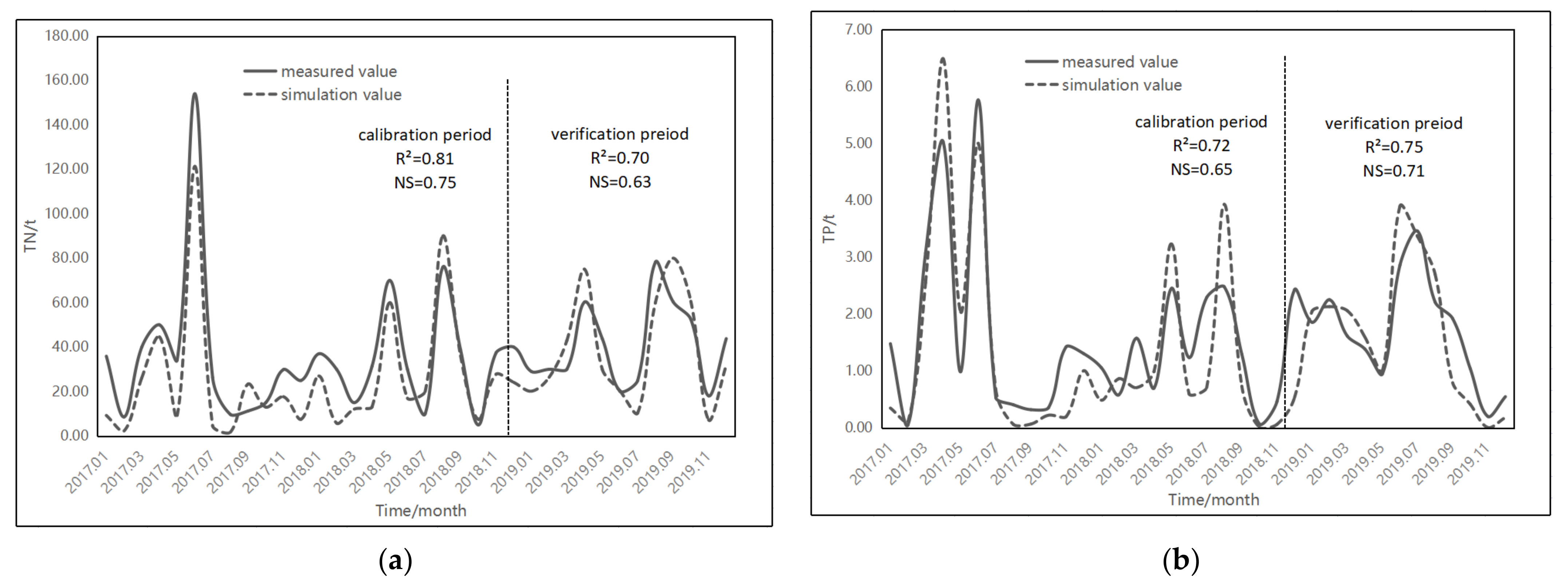
3.2.2. Model Calibration and Validation

Five sensitive parameters were identified: ERORGN, NPERCO, SDNCO, PHOSKD, and PPERCO. Each sensitive parameter was manually calibrated, and the optimal values are listed in Table 6. The comparison of measured and simulation values in calibration and verification period is provided in Figure 4. During the calibration period, the R2 values of TN and TP were 0.81 and 0.72, respectively, and the NS values of TN and TP were 0.75 and 0.65, showing a close agreement between the measured and simulated values. During the verification period, the R2 values of TN and TP both reached 0.4 and met the criteria (for TN, R2 value was 0.7, and for TP, R2 value was 0.75), and the NS values of TN and TP both exceeded 0.35 and met the criteria (for TN, NS value was 0.63, and for TP, NS value was 0.71), which was considered acceptable and applicable for future application in this study.
For the average monthly TN value, the simulated value of 30.73 t is lower than the measured value of 37.21 t, and for the average monthly TP value, the simulated value of 1.64 t is lower than the measured value of 1.47 t. The reason for the underestimation is precipitation. Since these were wet years in the simulation period, strong rainfall runoff washed NPS pollutants into the river, making a small part of the pollution output remained in the soil and seepage pits. The coefficient of pollutants entering the river was relatively large.

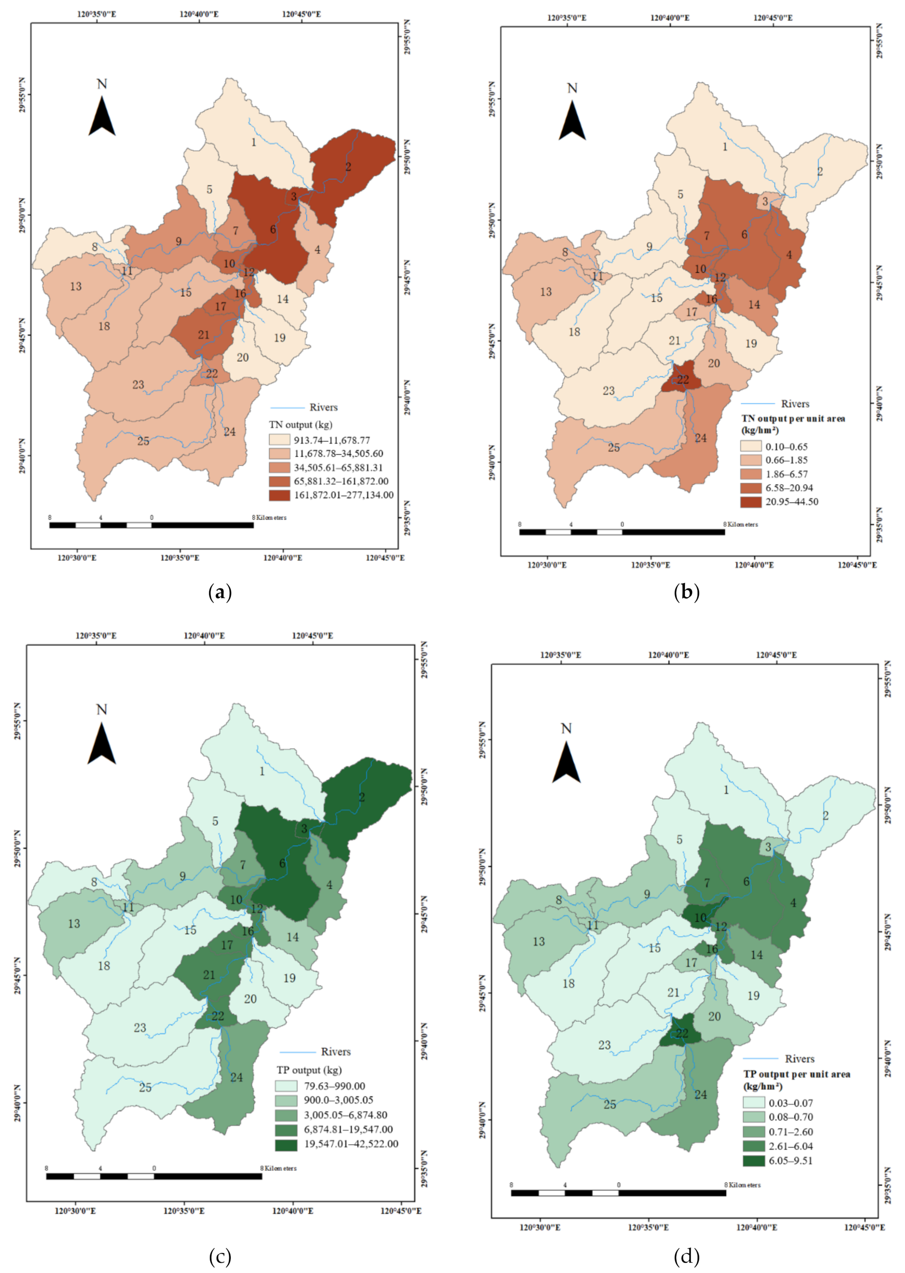
3.2.3. Spatial Variation Characteristics of TN&TP Output Simulated by SWAT

Under the simulated results of SWAT model, the annual TN&TP output in the whole study area is 300.87 t and 24.23 t, respectively, and the unit TN&TP output is 6.61 kg/hm2 and 0.53 kg/hm2, respectively.
Using the natural break point method, the output and output per unit area of TN&TP in the river section were divided into five categories (Figure 5). The TN&TP displayed similar spatial distribution characteristics. In terms of output and output per unit area, TN was always higher than TP. The TN&TP output were the highest at the junction of Southern Stream and Northern Stream, located in sub-basins 2, 3, and 6, and the TN&TP in the entire basin reached the maximum as the rivers merged. The second and third grades were mainly distributed near the river channels of Southern Stream (located in the sub-basins 10, 12, 16, 17, 21, and 22) and Northern Stream (located in the sub-basins 7, 9, and 11), respectively. The fourth grade was mainly located at the source of Southern Stream and Northern Stream, located in sub-basins 12, 18, 22, 23, 24, and 25. The slope of this area was larger, and with the surface runoff formed by rainfall washing into the river, the TN&TP attached to the sediment, causing the TN&TP to increase. The areas with the lowest TN&TP outputs were scattered in the basin. The areas with large TN&TP output per unit area were located in sub-basins 4, 10, 12, 15, and 22, where the cultivated land and construction land were concentrated and the landscape pattern was relatively complex.

3.3. Relationship between the Spatial Land Use/Cover Pattern and Water Quality

3.3.1. Differences in Land Use/Cover on TN&TP Output

The impact of different land use/cover types on the TN&TP output is explored in Table 7. The TN annual output from garden land contributed the most, accounting for 45.98%, followed by forest and cultivated land. Construction land had the lowest annual output, being only 0.94%. The TP annual output from cultivated land contributed the most, accounting for 44.55%, followed by forest garden land and construction land. From the perspective of the TN&TP output per unit area, the land use/cover types were ranked as follows in term of TN: garden land (18.83 kg/km2) > cultivated land (15.49 kg/km2) > forest (2.76 kg/km2) > construction land (1.92 kg/km2) and as follows in terms of TP: cultivated (2.15 kg/km2) > garden land (0.60 kg/km2) > construction land (0.32 kg/km2) > forest (0.28 kg/km2).

3.3.2. Differences in the Influences of Land Use/Cover on TN&TP among the Scales

The rivers in each sub-basin were divided into six spatial buffer scales of 100 m, 300 m, 500 m, 700 m, 1000 m, and the whole catchment. Explore the impact of land use/cover types on TN&TP under different buffer zones using RDA. From the species–environment ranking of RDA (Figure 6), the distribution of species, the relationship between species and environmental factors, and the relationship between different environmental factors could be derived.
Regardless of the buffer zone, cultivated land and construction land were positively correlated with the TN&TP outputs. On the contrary, forest was negatively correlated with the TN&TP outputs. No matter under which buffer zone, the axes of the garden were almost perpendicular to the axes of TN&TP. Therefore, there was no significant relationship between the proportion of garden land and water area and the output of TN&TP.
The relationship between the output per unit area of TN&TP and land use/cover varied with the spatial scale. As the buffer size increased, the proportion of cultivated land area decreased. The angle between the axis of cultivated land and TN became larger, while that between cultivated land and TP become smaller from 100-m buffer to the whole catchment. That is to say, the correlation between the cultivated land and the TN output per unit area weakened, while the correlation with the TP output per unit area increased. For construction land, the proportion of its area gradually decreased as the buffer zone increased. The correlation between construction land and TN&TP per unit area reached the maximum in the buffer range of 100 m buffer scale, and the correlation was weaker at other buffer scales. The proportion of forest area increased with the increase of the buffer zone. The forest had an increased negative correlation with the TN&TP output per unit area at the buffer scale from 100 m to 500 m. The correlation between forest and TN&TP summited at the buffer scales of 500–700 m, after which the negative correlation began to weaken as it became larger than the 700-m buffer scale.

3.3.3. The Impact of Landscape Pattern on TN&TP

The water quality change of the river basin was closely related to the composition of the landscape pattern. In this study, the landscape pattern index and the TN&TP inflow into the river in the sub-basin were used as environmental factors and species variables to explore the impact of the landscape pattern index on the output of TN&TP. Note from Table 8 that the characteristic value of the A1 principal axis of the RDA ranking was 0.731, and the interpretation amount was 73.1%. The correlation coefficients of the A1 principal axis and the A2 principal axis were 0.857 and 0.839, respectively, indicating that the landscape pattern of the Tang-Pu Reservoir basin was related to the output of TN&TP.
To further verify the relevance of each landscape pattern factor to the TN&TP output, a t-value double sequence diagram was made for the results of the RDA (Figure 7). The results showed that SHDI and CONTAG had a greater impact on TN&TP. IJI, SPLIT, SHDI, and DIVISION had a strong positive correlation with the output of TN&TP. The larger the SPLIT, IJI, DIVISION, and SHDI, the higher the fragmentation and separation of the landscape and the richer the basin landscape, which may increase the output of TN&TP. There was a certain negative correlation between LPI, CONTAG, and AI and the output of TN&TP. Larger LPI, CONTAG, and AI indicated better landscape integrity and connectivity among landscape patches. It showed that there was less interference from human activities, resulting in a lower degree of landscape fragmentation, so the TN&TP output decreased. In addition, the correlation between the other indexes and the TN&TP output was not very strong.

4. Discussion

4.1. Relationship between Land Use/Cover and TN&TP

Land use/cover types and their spatial distribution affect the water pollution status of water bodies at the basin [4,10,16]. Owing to differences in land use/cover patterns and human activity intensity, they can be significantly correlated, i.e., different land use/cover types have different pollutant outputs [45]. During rainfall, surface pollutants flow into the water with surface runoff, and pollutants may be deposited, absorbed, and reprecipitated when flowing through different land use/cover types [46].
This study showed that construction land and cultivated land had negative effects on water quality, whereas forest had positive effects on water quality. These results are consistent with most previous studies [6,47,48]. Regardless of the buffer zone, the construction land was positively correlated with the TN&TP outputs. The pollution in construction land is transferred to streams via runoff from impervious surfaces, which adversely affects stream water quality after rainfall runoff is washed away [49,50]. The limited construction land area in the Tang-Pu Reservoir basin is the main factor contributing to the poor TN&TP output. Cultivated land strongly influences the nutrient concentrations of stream water [51]. Owing to fertilization, pesticides, and agricultural management measures such as irrigation, the TN&TP output in cultivated land is relatively high, which causes eutrophication of the water during and following precipitation events [52,53].
The large area coverage of forest did not produce a large TN&TP output. Vegetation plays a positive role in soil and water conservation so that the N and P elements in the soil are lost less with surface runoff. That is to say, forest is considered as a sink for potential pollutants in water bodies [52,54]. This is also in line with some research results that the water quality of sub-basins dominated by forest is better than those dominated by cultivated land and garden land [16,55].

4.2. Scale Effect on the Influences of Land Use/Cover on TN&TP

The influence of land use/cover pattern on water quality is scale dependent [53,56,57]. Herein, different land use/cover patterns had various scale effects. For example, construction land had greater impacts on TN at smaller scales. This can be explained from two aspects. From the perspective of the nature of N, it may be due to the denitrification of part of the N under the action of microorganisms during the long-distance runoff transport of the N fertilizer applied to the cultivated land [58] or that the positively charged NH 4 + is easily absorbed by soil particles and used by plants. From the perspective of land use/cover structure, as the proportion of forest increases, forest intercepts some of the TN generated by agricultural activities. As a result, the correlation between TN and cultivated land becomes worse as the buffer size increases [54,55]. Construction land was more strongly correlated with TN&TP at smaller scales. This may be related to the distribution of rural residential land along the river and the artificial disturbances, which greatly damage river ecosystems. Forest was highly correlated with improved water quality at the buffer scale of 500–700 m. The wider the riparian zone, the greater the effect of intercepting pollutants [59]. Riparian vegetation plays an important role in maintaining and improving water quality [60]. These findings showed that the area of cultivated land and construction land should be reduced in the buffer zone closer to the river, while the application of fertilizers in cultivated land should be reduced. And the area of forest land should be increased in the buffer zone of 500–700 m to intercept N and P elements.
The complexity of the scale effects indicates how challenging it is to select a single optimal scale to control a large number of water quality parameters because of the different biogeochemical processes occurring at different scales [61]. Therefore, a multi-scale perspective should be provided for sustainable utilization of water resources and land use/cover planning. In exploring the relevance of land use/cover and water quality, the result is not only affected by the proportion of land use/cover area but also by the spatial pattern of land use/cover to a certain extent; that is to say, the patch fragmentation and spatial interconnection of land use/covers played an important role in modulating land use/cover effects on water quality in this study, as supported by several studies [62,63]. Sun et al. [64] found that an aggregated forest landscape had a greater ability to fix and absorb pollutants in streams than a dispersed forest landscape. This suggested that it might be possible to engineer a land use/cover configuration to improve water quality without appreciably altering the land use/cover composition in the study area.

4.3. Relationship between Landscape Pattern and TN&TP

The pattern and process theory of landscape ecology explains the spatial differences between water quality. One of the reasons is that water quality is a comprehensive reflection of multiple land use/cover composition and land use/cover spatial distribution [65]. Thus, when there is heterogeneity in different sub-basins, the degree of impact on the water quality of river also differs. Our landscape pattern conclusions were consistent with some previous studies, but there were also inconsistencies. For example, similar to the results of Lee et al. [66] and Shi et al. [53], water quality was positively correlated with SHDI and negatively correlated with CONTAG. The reason is that the height of SHDI represents the richness of diversity and heterogeneity of the landscape, which is related to the increase in the types of landscape patches, leading to a balanced distribution of various patch types [67]. It may also be related to the richness of patches and the complexity of the landscape structure [68]. CONTAG reflects the degree of separation and spread of the landscape. A high spread value indicated that a certain dominant patch type in the landscape has formed good connectivity, and the degree of fragmentation of the landscape is low. Obviously, for this study area where forest is the dominant landscape type, a high SHDI and low LPI indicate intense human interference, and the dominance of pollution source landscape types (i.e., construction land and cultivated land) will increase. The degree of fragmentation of forest will increase simultaneously, resulting in the increasing risk of water quality degradation. Contrary to our result, Sun et al. [69] and Zhang et al. [70] found that with the increase of SHDI, river water quality tended to be better, and at the same time, CONTAG was positively correlated with river water quality. The reason for this result may be related to the dominant species in the study area. The dominant landscape type of the study areas of Sun et al. [69] and Zhang et al. [70] were pollution source landscapes, that is, basins dominated by construction land or cultivated land. This is contrary to our study area, and therefore the higher the CONTAG, the more obvious the plaque aggregation and connectivity. It led to an increase in the concentration of pollutants in the water. The same applies for SHDI. In addition, the reason for the inconsistency of some results may be related to the research scale. Li et al. [71] studied the correlation between the landscape pattern and water quality from a series of spatial scales, and the results showed that it is at the sub-basin scale that CONTAG and the concentration index of various pollutants in water have a negative correlation, while SHDI is associated with a positive correlation. At other spatial scales, the result is the opposite.
In general, owing to differences in regional characteristics and spatial and temporal scales, the landscape index and water quality did not reach a unified conclusion and demonstrated many uncertainties, indicating that further landscape-water quality correlation research is needed.

4.4. Limitations

Some limitations should be noted in this study. First, due to the lack of long-term data in the basin, only one year of water quality was simulated by SWAT model. Thus, only the effect of land use/cover on the NPS pollution in 2019 was analyzed. Although the results of the relationship between land use/cover and TN&TP in 2019 remain consistent with most studies, it is recommended that more years need to be investigated to improve the confidence of the result. Second, the SWAT model can only simulate the spatial distribution of nutrient contamination in the basin but not the other water quality parameters, i.e., DO, EC, and COD Mn. TN&TP do not fully represent the water quality of the basin. Based on the study results, more spatial distribution of other water quality parameters can be simulated to explore the impact of land use/cover on water quality indicators.

5. Conclusions

A better understanding of the impact of land use/cover pattern on water quality could provide guidelines for NPS pollution caused by improper land use/cover to achieve sustainable water resources utilization. Although SWAT model can simulate the TN&TP output to display the overall NPS pollution situation in entire basin, its results were rarely used to explore the influence of land use/cover and landscape pattern on water quality. Based on the outcomes of monitoring the land use/cover pattern and assessing the water quality in the Tang-Pu Reservoir basin, our study simulated the output values and their spatial distribution of the most influencing factors for water quality, that is, the TN&TP, and explored the correlations between land use/cover pattern and TN&TP output by the redundancy analysis.
We found that the land use/cover type was little affected between the period 2009 and 2019. Forest was the dominant land cover, displaying a decreasing tendency. Constructed land exhibited the most obvious change, occupying the surrounding cultivated land, and cultivated land was decreasing in the basin. The landscape fragmentation increased, and the connectivity decreased. The assessment characterized the water quality showed that TN&TP was the most influencing factor, and the high N and P pollution in the reservoir contributed a great deal to the eutrophication problems. Under the simulation of SWAT, the TN&TP outputs were highest at the junction of rivers, and the output per unit TN&TP was at the areas where the landscape pattern was highly fragile. We also found that owing to fertilization, pesticides, and agricultural management measures, i.e., irrigation, the output per unit area TN&TP of cultivated land and garden land was higher than that of construction land and forest. There existed a positive correlation between the TN&TP and cultivated land and construction land, which means that the expansion of cultivated land and construction land inevitably increased the NPS pollution in the basin. Vegetation plays a positive role in soil and water conservation so that the N and P elements in the soil are lost less with surface runoff. Meanwhile, different land use/cover types had different scale effects. The correlation between forest and TN&TP summited at 500–700-m buffer and construction land at 100-m buffer. As the buffer size increased, the correlation between the cultivated land and the TN weakened, while the correlation with the TP increased. These findings indicated that land use/cover planning in water quality management needs to adopt a multi-scale perspective. The TN&TP outputs in the sub-basin were positively correlated with SHDI and negatively correlated with CONTAG in the area where forest is the dominant land cover. Therefore, the area of cultivated land and construction land should be reduced in the buffer zone closer to the river, and the application of fertilizers in cultivated land should be reduced. The more connected forest land should be increased in the 500–700-m buffer zone to intercept N and P elements. These will be necessary to promote sustainable water resources utilization.

Author Contributions

All authors contributed to results interpretation and paper writing. K.L.: data curation, formal analysis, methodology, writing—original draft. Y.W.: methodology, software, data curation. F.L.: software, writing—review and editing. J.Y.: investigation, visualization. M.X.: validation, visualization. Y.L. (Yi Li): supervision, visualization. Y.L. (Yan Li): conceptualization, funding acquisition, resources, writing—review and editing. All authors have read and agreed to the published version of the manuscript.

Funding

This work was financed by the National Natural Science Foundation of China (Grants No. 41771244; 72004014); the Key Program of Zhejiang Provincial Natural Science Foundation of China (LZ21D010002); and The National Key Research and Development Program of China (2016YFD0201200).

Data Availability Statement

All data generated or analyzed during this study are included in this published article.

Conflicts of Interest

The authors declare no competing interest.

References

  1. Lu, Y.; Song, S.; Wang, R.; Liu, Z.; Meng, J.; Sweetman, A.; Jenkins, A.; Ferrier, R.C.; Li, H.; Luo, W.; et al. Impacts of soil and water pollution on food safety and health risks in China. Environ. Int. 2015, 77, 5–15. [Google Scholar] [CrossRef] [PubMed] [Green Version]
  2. Ou, Y.; Wang, X.; Wang, L.; Rousseau, A.N. Landscape influences on water quality in riparian buffer zone of drinking water source area, northern China. Environ. Earth Sci. 2016, 75, 114. [Google Scholar] [CrossRef]
  3. Sener, S.; Davraz, A.; Karaguezel, R. Evaluating the anthropogenic and geologic impacts on water quality of the Eirdir lake, turkey. Environ. Earth Sci. 2013, 70, 2527–2544. [Google Scholar] [CrossRef]
  4. You, Q.; Fang, N.; Liu, L.; Yang, W.; Zhang, L.; Wang, Y. Effects of land use, topography, climate and socio-economic factors on geographical variation pattern of inland surface water quality in China. PLoS ONE 2019, 14, e0217840. [Google Scholar] [CrossRef]
  5. Ongley, E.D.; Zhang, X.; Yu, T. Current status of agricultural and rural non-point source pollution assessment in China. Environ. Pollut. 2010, 158, 1159–1168. [Google Scholar] [CrossRef] [PubMed]
  6. Tu, J. Spatially varying relationships between land use and water quality across an urbanization gradient explored by geographically weighted regression. Appl. Geogr. 2011, 31, 376–392. [Google Scholar] [CrossRef]
  7. Wilson, C.; Weng, R. Assessing surface water quality and its relation with urban land cover changes in the lake calumet area, greater Chicago. Environ. Manag. 2010, 45, 1096–1111. [Google Scholar] [CrossRef]
  8. Johnson, L.; Richards, C.; Host, G.; Arthur, J. Landscape influences on water chemistry in midwestern stream ecosystems. Freshw. Biol. 1997, 37, 193–208. [Google Scholar] [CrossRef]
  9. Castillo, M.; Morales, H.; Valencia, E.; Morales, J.; Cruz-Motta, J. The effects of human land use on flow regime and water chemistry of headwater streams in the highlands of Chiapas. Knowl. Manag. Aquat. Ecosyst. 2012, 347, 135–152. [Google Scholar] [CrossRef] [Green Version]
  10. Mirhosseini, M.; Farshchi, P.; Noroozi, A.A.; Shariat, M.; Aalesheikh, A.A. Changing land use a threat to surface water quality: A vulnerability assessment approach in Zanjanroud Watershed, Central Iran. Water Resour. 2018, 45, 268–279. [Google Scholar] [CrossRef]
  11. Gu, Q.; Hu, H.; Ma, L.; Sheng, L.; Yang, S.; Zhang, X.; Zhang, M.; Zheng, K.; Chen, L. Characterizing the spatial variations of the relationship between land use and surface water quality using self-organizing map approach. Ecol. Indic. 2019, 102, 633–643. [Google Scholar] [CrossRef]
  12. Valle, R.F.; Varanda, S.; Fernandes, L.; Pacheco, F.A.L.; Junior, R.V. Groundwater quality in rural watersheds with environmental land use conflicts. Sci. Total Environ. 2014, 485–486, 110–120. [Google Scholar] [CrossRef]
  13. Pacheco, F.A.L.; Fernandes, L.S. Environmental land use conflicts in catchments: A major cause of amplified nitrate in river water. Sci. Total. Environ. 2016, 548, 173–188. [Google Scholar] [CrossRef] [PubMed]
  14. Rodrigues, V.; Estrany, J.; Ranzini, M.; de Cicco, V.; Martin-Benito, J.M.T.; Hedo, J.; Lucas-Borja, M.E. Effects of land use and seasonality on stream water quality in a small tropical catchment: The headwater of Córrego Água Limpa, São Paulo (Brazil). Sci. Total. Environ. 2018, 622–623, 1553–1561. [Google Scholar] [CrossRef] [Green Version]
  15. Patino, R.; Asquith, W.H.; VanLandeghem, M.M.; Dawson, D. Long-term trends in reservoir water quality and quantity in two major river basins of the southern great plains. Lake Reserv. Manag. 2015, 31, 254–279. [Google Scholar] [CrossRef]
  16. Mello, K.; Valente, R.A.; Randhir, T.O.; dos Santos, A.C.A.; Vettorazzi, C.A. Effects of land use and land cover on water quality of low-order streams in southeastern brazil: Watershed versus riparian zone. Catena 2018, 167, 130–138. [Google Scholar] [CrossRef]
  17. Xu, J.; Jin, G.; Tang, H.; Mo, Y.; Wang, Y.-G.; Li, L. Response of water quality to land use and sewage outfalls in different seasons. Sci. Total. Environ. 2019, 696, 134014. [Google Scholar] [CrossRef]
  18. Xiao, R.; Wang, G.; Zhang, Q.; Zhang, Z. Multi-scale analysis of relationship between landscape pattern and urban river water quality in different seasons. Sci. Rep. 2016, 6, 25250. [Google Scholar] [CrossRef] [Green Version]
  19. Casquin, A.; Dupas, R.; Gu, S.; Couic, E.; Gruau, G.; Durand, P. The Influence of Landscape Spatial Configuration on Nitrogen and Phosphorus Exports in Agricultural Catchments. 2021. Available online: https://link.springer.com/article/10.1007/s10980-021-01308-5 (accessed on 25 July 2021).
  20. Simsek, D.; Sertel, E. Spatial analysis of two different urban landscapes using satellite images and landscape metrics. Photogramm. Eng. Remote. Sens. 2018, 84, 711–721. [Google Scholar] [CrossRef]
  21. Ding, J.; Jiang, Y.; Liu, Q.; Hou, Z.; Liao, J.; Fu, L.; Peng, Q. Influences of the land use pattern on water quality in low-order streams of the Dongjiang River basin, China: A multi-scale analysis. Sci. Total. Environ. 2016, 551–552, 205–216. [Google Scholar] [CrossRef]
  22. Janardan, M.; Chang, H. Landscape and anthropogenic factors affecting spatial patterns of water quality trends in a large river basin, south Korea. J. Hydrol. 2018, 564, 26–40. [Google Scholar] [CrossRef]
  23. Arnold, J.G.; Srinivasan, R.; Muttiah, R.S.; Williams, J.R. Large area hydrologic modeling and assessment part i: Model development. AWRA J. Am. Water Resour. Assoc. 1998, 34, 73–89. [Google Scholar] [CrossRef]
  24. Zhang, C.; Li, S.; Qi, J.; Xing, Z.; Meng, F. Assessing impacts of riparian buffer zones on sediment and nutrient loadings into streams at watershed scale using an integrated REMM-SWAT model. Hydrol. Process. 2017, 31, 916–924. [Google Scholar] [CrossRef]
  25. Sertel, E.; Imamoglu, M.Z.; Cuceloglu, G.; Erturk, A. Impacts of land cover/use changes on hydrological processes in a rapidly urbanizing mid-latitude water supply catchment. Water 2019, 11, 1075. [Google Scholar] [CrossRef] [Green Version]
  26. Andrianaki, M.; Shrestha, J.; Kobierska, F.; Nikolaidis, N.P.; Bernasconi, S.M. Assessment of SWAT spatial and temporal transferability for a high-altitude glacierized catchment. Hydrol. Earth Syst. Sci. 2019, 23, 3219–3232. [Google Scholar] [CrossRef] [Green Version]
  27. Meng, F.; Sa, C.; Liu, T.; Luo, M.; Liu, J.; Tian, L. Improved model parameter transferability method for hydrological simulation with SWAT in Ungauged Mountainous Catchments. Sustainability 2020, 12, 3551–3569. [Google Scholar] [CrossRef]
  28. Zeiger, S.; Owe, M.R.; Pavlowsk, R.T. Simulating nonpoint source pollutant loading in a karst basin: A swat modeling application. Sci. Total. Environ. 2021, 785, 147295. [Google Scholar] [CrossRef]
  29. Fan, M.; Shibata, H. Simulation of watershed hydrology and stream water quality under land use/cover and climate change scenarios in Teshio River watershed, northern Japan. Ecol. Indic. 2015, 50, 79–89. [Google Scholar] [CrossRef]
  30. Gashaw, T.; Tulu, T.; Argaw, M.; Worqlul, A.W. Modeling the hydrological impacts of land use/cover/land cover changes in the Andassa watershed, Blue Nile Basin, Ethiopia. Sci. Total. Environ. 2018, 619–620, 1394–1408. [Google Scholar] [CrossRef]
  31. Dai, X.; Zhou, Y.; Ma, W.; Zhou, L. Influence of spatial variation in land use patterns and topography on water quality of the rivers inflowing to Fuxian Lake, a large deep lake in the plateau of southwestern China. Ecol. Eng. 2017, 99, 417–428. [Google Scholar] [CrossRef]
  32. Qian, Y.; Sun, L.; Chen, D.; Liao, J.; Tang, L.; Sun, Q. The response of the migration of non-point source pollution to land use change in a typical small watershed in a semi-urbanized area. Sci. Total. Environ. 2021, 785, 147387. [Google Scholar] [CrossRef]
  33. Xiaoyan, Z.; Yan, S.; Haijiang, C.; Xiaofang, H. Study on water quality of Tangpu Reservoir for drinking water supply in Shaoxing City. Water Wastewater Eng. 2008, 34, 38–42. [Google Scholar] [CrossRef]
  34. Chaplot, V. Impact of DEM mesh size and soil map scale on SWAT runoff, sediment, and NO3–N loads predictions. J. Hydrol. 2005, 312, 207–222. [Google Scholar] [CrossRef]
  35. Pal, M. Random forests for land cover classification. In Proceedings of the IEEE International Geoscience & Remote Sensing Symposium, Toulouse, France, 21–25 July 2003; IEEE: New York, NY, USA, 2004. [Google Scholar]
  36. Chan, C.W.; Paelinckx, D. Evaluation of Random Forest and Adaboost tree-based ensemble classification and spectral band selection for ecotope mapping using airborne hyperspectral imagery. Remote Sens. Environ. 2008, 112, 2999–3011. [Google Scholar] [CrossRef]
  37. Anand, J.; Gosain, A.K.; Khosa, R. Prediction of land use changes based on land change modeler and attribution of changes in the water balance of ganga basin to land use change using the swat model. Sci. Total. Environ. 2018, 644, 503–519. [Google Scholar] [CrossRef] [PubMed]
  38. Lin, B.; Chen, X.; Yao, H.; Chen, Y.; Liu, M.; Gao, L.; James, A. Analyses of landuse change impacts on catchment runoff using different time indicators based on swat model. Ecol. Indic. 2015, 58, 55–63. [Google Scholar] [CrossRef]
  39. Shen, Z.; Qiu, J.; Hong, Q.; Chen, L. Simulation of spatial and temporal distributions of non-point source pollution load in the three gorges reservoir region. Sci. Total. Environ. 2014, 493, 138–146. [Google Scholar] [CrossRef]
  40. Moriasi, D.; Gitau, M.; Pai, N.; Daggupati, P. Hydrologic and water quality models: Performance measures and evaluation criteria. Trans. Asabe 2015, 58, 1763–1785. [Google Scholar] [CrossRef] [Green Version]
  41. Shen, Z.; Hou, X.; Li, W.; Aini, G.; Chen, L.; Gong, Y. Impact of landscape pattern at multiple spatial scales on water quality: A case study in a typical urbanised watershed in China. Ecol. Indic. 2015, 48, 417–427. [Google Scholar] [CrossRef]
  42. Liu, H.; Meng, C.; Wang, Y.; Li, Y.; Li, Y.; Wu, J. From landscape perspective to determine joint effect of land use, soil, and topography on seasonal stream water quality in subtropical agricultural catchments. Sci. Total. Environ. 2021, 783, 147047. [Google Scholar] [CrossRef]
  43. Zhao, J.; Lin, L.; Yang, K.; Liu, Q.; Qian, G. Influences of land use on water quality in a reticular river network area: A case study in Shanghai, China. Landsc. Urban Plan. 2015, 137, 20–29. [Google Scholar] [CrossRef]
  44. Chinese State Environment Protection Bureau. 2002 Environmental Quality Standards for Surface Water (GB3838-2002); Chinese State Environment Protection Bureau: Beijing, China, 2002. [Google Scholar]
  45. Yadav, S.; Babel, M.S.; Shrestha, S.; Deb, P. Land use impact on the water quality of large tropical river: Mun River basin, Thailand. Environ. Monit. Assess. 2019, 191, 614. [Google Scholar] [CrossRef]
  46. Yang, L.; Ma, K.M.; Guo, Q.H.; Zhao, J.Z.; Luo, Y.F. Zoning planning in non-point source pollution control in Hanyang district. Environ. Sci. 2006, 27, 31–36. [Google Scholar] [CrossRef]
  47. Song, Y.; Song, X.; Shao, G.; Hu, T. Effects of land use on stream water quality in the rapidly urbanized areas: A multiscale analysis. Water 2020, 12, 1123. [Google Scholar] [CrossRef] [Green Version]
  48. Wan, R.; Cai, S.; Li, H.; Yang, G.; Li, Z.; Nie, X. Inferring land use and land cover impact on stream water quality using a Bayesian hierarchical modeling approach in the Xitiaoxi River Watershed, China. J. Environ. Manag. 2014, 133, 1–11. [Google Scholar] [CrossRef]
  49. Johnson, R.C.; Jin, H.-S.; Carreiro, M.M.; Jack, J.D. Macroinvertebrate community structure, secondary production and trophic-level dynamics in urban streams affected by non-point-source pollution. Freshw. Biol. 2013, 58, 843–857. [Google Scholar] [CrossRef]
  50. Kraemer, S.A.; da Costa, N.B.; Shapiro, B.J.; Fradette, M.; Huot, Y.; Walsh, D.A. A large-scale assessment of lakes reveals a pervasive signal of land use on bacterial communities. ISME J. 2020, 14, 3011–3023. [Google Scholar] [CrossRef]
  51. Guo, M.; Zhang, T.; Li, J.; Li, Z.; Xu, G.; Yang, R. Reducing nitrogen and phosphorus losses from different crop types in the water source area of the Danjiang River, China. Int. J. Environ. Res. Public Health 2019, 16, 3442. [Google Scholar] [CrossRef] [PubMed] [Green Version]
  52. Räty, M.; Järvenranta, K.; Saarijärvi, E.; Koskiaho, J.; Virkajärvi, P. Losses of phosphorus, nitrogen, dissolved organic carbon and soil from a small agricultural and forested catchment in east-central Finland. Agric. Ecosyst. Environ. 2020, 302, 107075. [Google Scholar] [CrossRef]
  53. Shi, P.; Zhang, Y.; Li, Z.; Li, P.; Xu, G. Influence of land use and land cover patterns on seasonal water quality at multi-spatial scales. Catena 2017, 151, 182–190. [Google Scholar] [CrossRef]
  54. Bahar, M.; Ohmori, H.; Yamamuro, M. Relationship between river water quality and in a small river basin running through the urbanizing area of central Japan. Limnology 2008, 9, 19–26. [Google Scholar] [CrossRef]
  55. Ye, Y.; He, X.; Chen, W.; Yao, J.; Yu, S.; Jia, L. Seasonal water quality upstream of Dahuofang reservoir, China-the effects of land use type at various spatial scales. CLEAN Soil Air Water 2014, 42, 1423–1432. [Google Scholar] [CrossRef]
  56. Bian, Z.; Liu, L.; Ding, S. Correlation between spatial-temporal variation in landscape patterns and surface water quality: A case study in the Yi River Watershed, China. Appl. Sci. 2019, 9, 1053. [Google Scholar] [CrossRef] [Green Version]
  57. Pratt, B.; Chang, H. Effects of land cover, topography, and built structure on seasonal water quality at multiple spatial scales. J. Hazard. Mater. 2012, 209–210, 48–58. [Google Scholar] [CrossRef] [PubMed]
  58. Huang, J.; Li, Q.; Pontius, R.G.; Klemas, V.; Hong, H. Detecting the dynamic linkage between landscape characteristics and water quality in a subtropical coastal watershed, southeast China. Environ. Manag. 2013, 51, 32–44. [Google Scholar] [CrossRef] [PubMed]
  59. Fernandes, J.N.; Souza, A.L.T.; Tanaka, M.O. Can the structure of a riparian forest remnant influence stream water quality? A tropical case study. Hydrobiologia 2014, 724, 175–185. [Google Scholar] [CrossRef]
  60. De Souza, A.L.; Fonseca, D.G.; Libório, R.A.; Tanaka, M. Influence of riparian vegetation and forest structure on the water quality of rural low-order streams in SE Brazil. For. Ecol. Manag. 2013, 298, 12–18. [Google Scholar] [CrossRef]
  61. Meyer, J.L.; Strayer, D.L.; Wallace, J.B.; Eggert, S.L.; Helfman, G.S.; Leonard, N.E. The contribution of headwater streams to biodiversity in river networks. JAWRA J. Am. Water Resour. Assoc. 2007, 43, 86–103. [Google Scholar] [CrossRef] [Green Version]
  62. Uuemaa, E.; Roosaare, J.; Mander, Ü. Landscape metrics as indicators of river water quality at catchment scale. Nordic Hydrology 2007, 38, 125–138. [Google Scholar] [CrossRef]
  63. Gémesi, Z.; Downing, J.A.; Cruse, R.M.; Anderson, P.F. Effects of watershed configuration and composition on downstream lake water quality. J. Environ. Qual. 2011, 40, 517–527. [Google Scholar] [CrossRef] [PubMed]
  64. Sun, R.; Chen, L.; Chen, W.; Ji, Y. Effect of land use patterns on total nitrogen concentration in the upstream regions of the Haihe river basin, China. Environ. Manag. 2011, 51, 45–58. [Google Scholar] [CrossRef]
  65. Zhang, J.; Li, S.; Dong, R.; Jiang, C.; Ni, M. Influences of land use metrics at multi-spatial scales on seasonal water quality: A case study of river systems in the Three Gorges Reservoir Area, China. J. Clean. Prod. 2019, 206, 76–85. [Google Scholar] [CrossRef]
  66. Lee, S.-W.; Hwang, S.-J.; Lee, S.-B.; Hwang, H.-S.; Sung, H.-C. Landscape ecological approach to the relationships of land use patterns in watersheds to water quality characteristics. Landsc. Urban Plan. 2009, 92, 80–89. [Google Scholar] [CrossRef]
  67. Wu, J. Key concepts and research topics in landscape ecology revisited: 30 years after the Allerton Park workshop. Landsc. Ecol. 2013, 28, 1–11. [Google Scholar] [CrossRef]
  68. Osborne, L.L.; Wiley, M.J. Empirical relationships between land use/cover and stream water quality in an agricultural watershed. J. Environ. Manag. 1988, 26, 9–27. [Google Scholar] [CrossRef]
  69. Sun, Q.; Huang, J.; Hong, H.; Li, Q.; Feng, Y. Analysis on linkage between farm landscape and water quality in Jiulong river watershed. Trans. Chin. Soc. Agric. Eng. 2011, 27, 54–59. [Google Scholar] [CrossRef]
  70. Zhang, D.; Li, Y.; Sun, X.; Zhang, F.S.; Zhu, H.X.; Liu, Y.; Zhang, Y.; Zhuang, M.; Zhu, X.D. Relationship between landscape pattern and river water quality in Wujingang region, Taihu Lake watershed. Environ. Sci. 2010, 31, 1775–1783. [Google Scholar] [CrossRef]
  71. Li, Y.; Xu, Z.; Li, Y. A preliminary study on the relationship between multi-scale land use & landscape and river water quality response in the huntai watershed. Earth Environ. 2012, 40, 573–583. [Google Scholar]
Figure 1. The location of study area and the sampling sites in the Tang-Pu Reservoir basin, China.
Sustainability 13 11067 g001
Figure 4. Result of model calibration and validation. (a) Comparison of measured and simulated TN values during calibration and verification period in the Tang-Pu Reservoir; (b) comparison of measured and simulated TP values during calibration and verification period in the Tang-Pu Reservoir; (c) scatterplot between measured values and simulated values in calibration period; and (d) scatterplot between measured values and simulated values in verification period.
Sustainability 13 11067 g004aSustainability 13 11067 g004b
Figure 5. Spatial distribution of TN&TP output and output per unit area in sub-basin. (a) TN output; (b) TN output per unit area; (c) TP output; and (d) TP output per unit area.
Sustainability 13 11067 g005
Figure 6. RDA analysis diagram in different buffer zones and proportion of land use/cover types. (a) Correlation between land use/cover factors and TN& TP (t-value) in 100 m; (b) in 300 m; (c) in 500 m; (d) in 700 m; (e) in 1000 m; and (f) in the whole catchment. The blue arrow indicates the species, that is, the output per unit of TN&TP, and the red arrow indicates the environmental factor, that is, the proportion of the five land categories. A positive correlation is expected when the arrows of the two variables point in the same direction and vice versa. (g) Proportion of land use/cover types under different buffer zones.
Sustainability 13 11067 g006
Figure 7. Correlation between landscape metrics and TN& TP (t-value). (a) Correlation between landscape metrics and TN; (b) correlation between landscape metrics and TP; if the arrow of a certain environment completely falls on a blue circle, it indicates that it is significantly positively correlated with the species. Oppositely, if the arrow of a certain environmental factor falls within the red circle, it indicates that the species and the environmental factor are significantly negatively correlated. The more the arrow falls within a circle, the more significant the correlation between the species and the environmental factor.
Sustainability 13 11067 g007
Table 1. Data description and source.
Data TypeSourceResolutionYear
Landsat 5 TM images Surface Reflectance Tier 1
(path 118 and row 39)
GEE (https://http://earthengine.google.com/)
(accessed on 1 Feburary 2021)
30 m2009.10
Landsat 8 OLI images Surface Reflectance Tier 1
(path 118 and row 39)
GEE (https://http://earthengine.google.com/)
(accessed on 1 Feburary 2021)
30 m2019.10
DEMGeospatial Data Cloud (http://www.gscloud.cn/)
(accessed on 1 Feburary 2021)
12.5 m2019
SoilHarmonized World Soil Database1 km2010
Digital land use/cover mapsLand use change survey from Shaoxing Ecological Environment Bureau/2019
Meteorological dataShaoxing meteorological stationsDaily2015–2019
Water quality parameters (TEM, DO, EC, TN, TP, and COD Mn)Shuang-Jiang Stream and Spillway Monitoring stationMonthly2017–2019
The hydrological dataShuang-Jiang Stream monitoring stationMonthly2015–2019
Management informationLocal statistics yearbook (http://www.stats.gov.cn/)
(accessed on 1 Feburary 2021)
Annual2019
Table 2. Descriptions of land use/cover types and landscape pattern metrics.
MetricDefinitionDescription
PDPatch Density is the number of corresponding patches divided by total landscape area.Reflects the fragmentation of landscape.
LPIThe area of the largest patch of the corresponding patch type divided by total landscape area.A measure of dominance.
PAFRAC2 divided by the slope of regression line obtained by regressing the logarithm of patch area against the logarithm of patch perimeter.Reflects shape complexity across a range of patch sizes.
LSIThe sum of the entire landscape boundary and all edges within the landscape boundary divided by the total landscape area. Reflects the complex shape of the patches that make up the landscape.
DIVISION1 minus the sum of patch area divided by total landscape area, quantity squared, summed across all patches of the corresponding patch type.Reflects the contagion/interspersion of the landscape
SPLITSPLIT equals the total landscape area squared divided by the sum of patch area squared, summed across all patches of the corresponding patch type.SPLIT increases as the focal patch type is increasingly reduced in area and subdivided into smaller patches
CONTAGExtent to which patch types are aggregated or clumped as a percentage of the maximum possible.Reflects the degree of agglomeration or extension trend of different patch types.
SHDIThe number of different patch types and the proportional area distribution among patch types.Compares and analyzes landscape diversity and heterogeneity.
SHEISHEI equals minus the sum, across all patch types, of the proportional abundance of each patch type multiplied by that proportion, divided by the logarithm of the number of patch types.Analyzes the diversity of the landscape and reflects a landscape dominated by one or a few dominant patch types.
Table 3. Confusion matrix of classification on 2009.
Land Use/Cover Types12345User’s Accuracy (%)
Forest 121210087.50
Cultivated land 211930082.61
Garden land 321190182.61
Water 4000200100.00
Constructed land 500102095.24
Producer’s accuracy (%)87.5086.3679.17100.0095.24
Overall accuracy (%): 89.19Kappa coefficent: 0.86
Table 4. Confusion matrix of classification on 2019.
Land Use/Cover Types12345User’s Accuracy (%)
Forest 121210087.50
Cultivated land 201920090.48
Garden land 311200186.96
Water 4000190100.00
Constructed land 500112090.91
Producer’s accuracy (%)95.4586.3683.3395.0095.24
Overall accuracy (%): 90.83Kappa coefficent: 0.88
Table 5. Descriptive statistics for water quality parameters from the period 2017 to 2019.
ParametersNMeanVarianceSDCVMaximumMinimumKurtosisSkewness
T (°C)7220.4652.827.270.3632.509.40−1.34−0.02
pH727.510.540.740.109.345.400.580.59
EC (μs/cm)728.982.211.490.1712.186.52−1.050.18
DO (mg/L)720.040.000.030.690.120.011.141.22
COD Mn(mg/L)721.900.810.900.486.440.7711.362.88
TP (mg/L)720.040.000.030.690.120.011.141.22
TN (mg/L)722.370.720.850.365.750.754.791.75
Note: N represents the number of samples, SD represents the standard deviation, and CV represents the coefficient of variation.
Table 6. The sensitive parameter and their optimal value in the Tang-Pu Reservoir Basin.
VariableParametersDescription of ParameterOptimal Value
TNERORGNOrganic nitrogen enrichment ratio0.614
NPERCONirogen percolation cofficient0.06
SDNCODenitrification threshold water content0.199
TP‘PHOSKDPhosphorus soil partitioning coefficient159.55
PPERCOPhosphorus percolation coefficient14.15
Table 7. Average annual TN&TP inflows and unit inflows of different land use/cover types.
Cultivated LandGarden LandForestConstruction Land
TNAnnual output (t)77.70138.3582.002.83
Percentage of annual output (%)25.8245.9827.250.94
Unit output (kg/hm2)15.4918.832.761.92
Annual output (t)10.804.448.520.47
TPPercentage of annual output (%)44.5518.3435.161.95
Unit inflows (kg/hm2)2.150.600.280.32
Annual output (t)77.70138.3582.002.83
Table 8. Results of RDA for landscape pattern factors and TN, TP.
Variation IndexAxis1Axis2Axis3Axis4
Eigen values0.7310.000.2650.00
Interpretation of each sort axis (%)73.173.499.9100.0
Correlation coefficient0.8570.8390.0000.000
Cumulative interpretation (%)99.6100.0
Publisher’s Note: MDPI stays neutral with regard to jurisdictional claims in published maps and institutional affiliations.

