Mapping Urban Environmental Performance with Emerging Data Sources: A Case of Urban Greenery and Traffic Noise in Sydney, Australia

 , and
, and
Abstract
:1. Introduction
2. Methods and Data
2.1. Mapping Urban Greenery
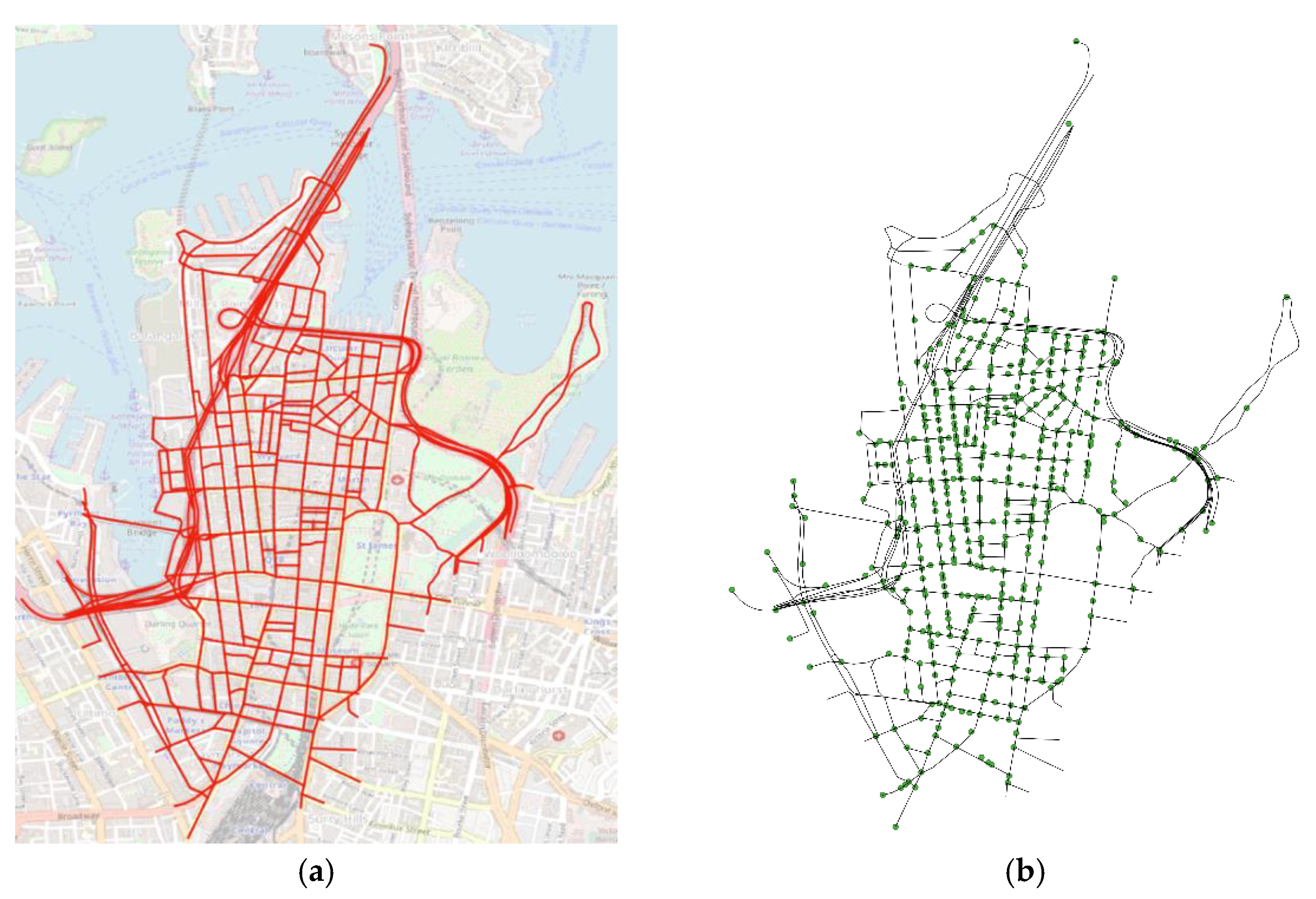
2.1.1. Location Sampling
2.1.2. Retrieving Metadata
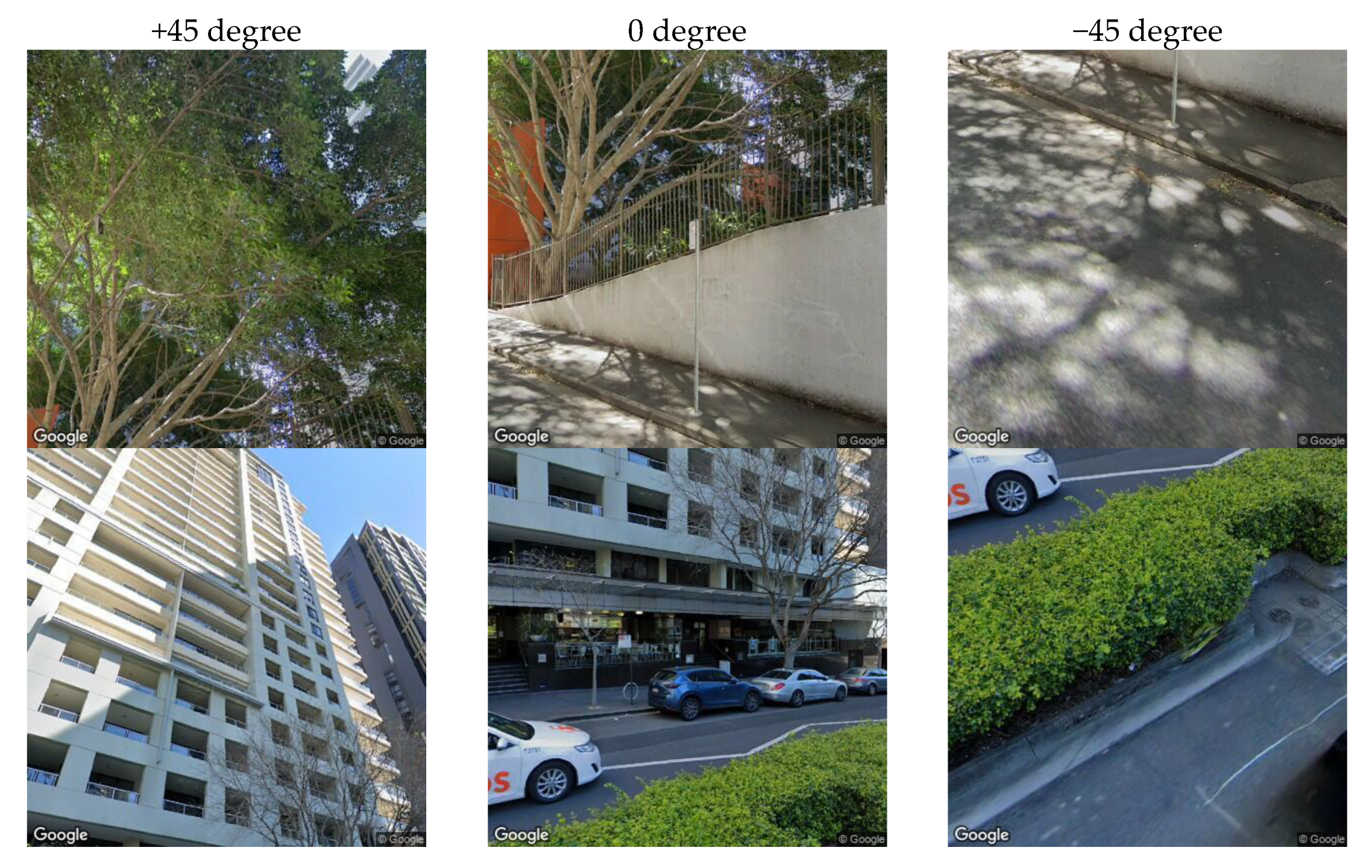
2.1.3. Calculating GVI using GSV Images
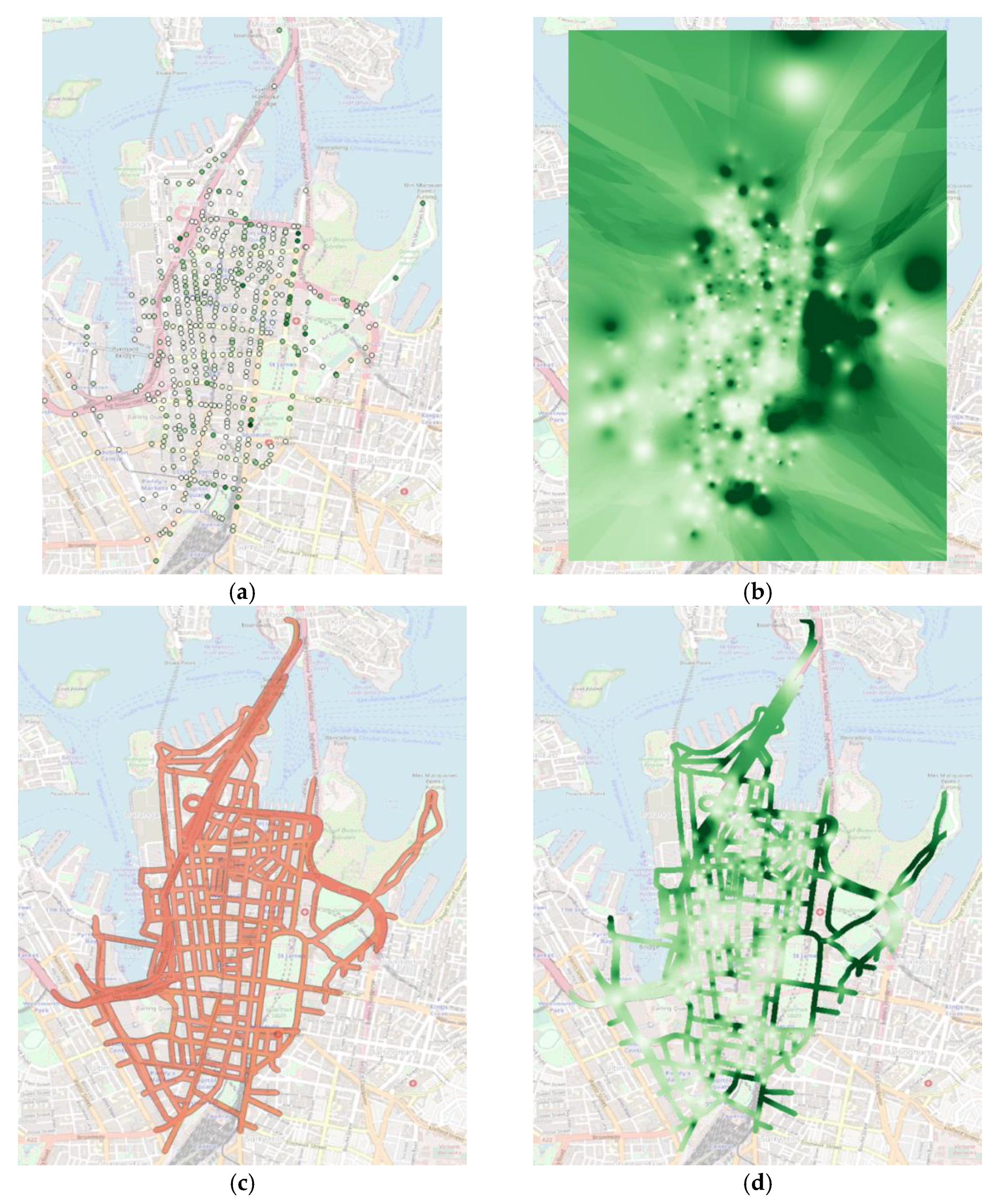
2.1.4. Visualization Techniques
2.2. Mapping Traffic Noise
2.2.1. Data Processing: Traffic Volumes and Building Footprints
2.2.2. Noise Propagation Model Parameter Calibration
- The maximum propagation distance which represents a cut-off distance between each source and receiver.
- The maximum wall seeking distance which permits overlooking walls farther than this distance between each source and receiver.
- The road width which represents an offset distance from the road center line to start creating receivers.
- The receiver’s densification value which creates additional receivers at this distance from sources.
- The maximum area of the triangle which sets the maximum surface for the noise map triangular mesh.
- The sound reflection order which represents the maximum number of wall reflections between each source and receiver.
- The sound diffraction order which represents the maximum number of horizontal diffractions between each source and receiver.
- The wall absorption value which indicates the level of noise absorption by the wall.
3. Results
3.1. Urban Greenery
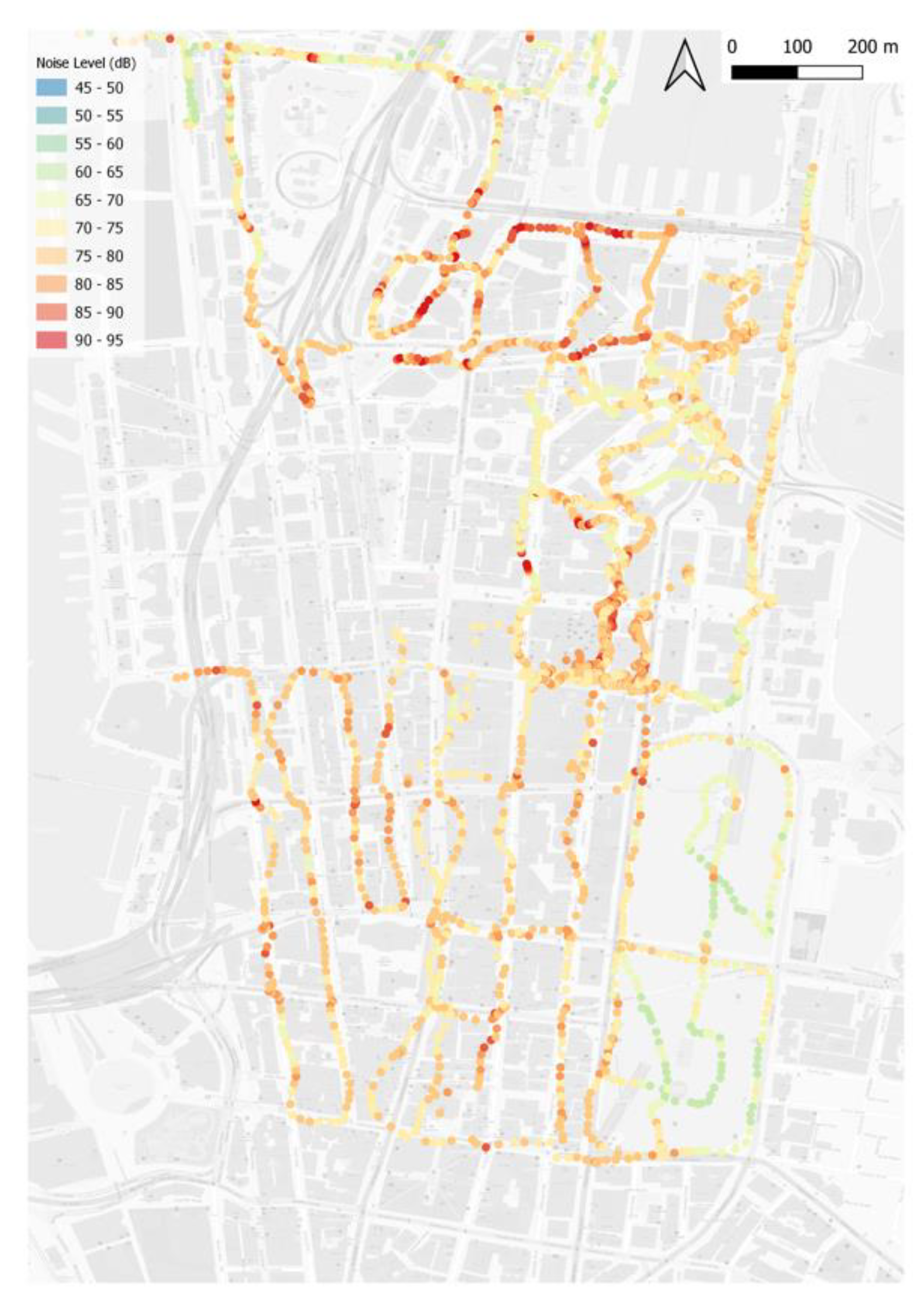
3.2. Traffic Noise
3.3. Spatio-Temporal Correlation between Urban Greenery and Traffic Noise
4. Conclusions
Author Contributions
Funding
Institutional Review Board Statement
Informed Consent Statement
Data Availability Statement
Acknowledgments
Conflicts of Interest
Appendix A
Appendix B

References
- Heaviside, C.; Macintyre, H.; Vardoulakis, S. The urban heat island: Implications for health in a changing environment. Curr. Environ. Health Rep. 2017, 4, 296–305. [Google Scholar] [CrossRef] [PubMed]
- Rich, J.H.; Nielsen, O.A. Assessment of traffic noise impact. Int. J. Environ. Stud. 2004, 61, 19–29. [Google Scholar] [CrossRef]
- Hammer, M.S.; Swinburn, T.K.; Neitzel, R.L. Environmental noise pollution in the United States: Developing an effective public health response. Environ. Health Perspect. 2014, 122, 115–119. [Google Scholar] [CrossRef] [PubMed] [Green Version]
- Badach, J.; Dymnicka, M.; Baranowski, A. Urban vegetation in air quality management: A review and policy framework. Sustainability 2020, 12, 1258. [Google Scholar] [CrossRef] [Green Version]
- Hwang, Y.H.; Nasution, I.K.; Amonkar, D.; Hahs, A. Urban green space distribution related to land values in fast-growing megacities, Mumbai and Jakarta-unexploited opportunities to increase access to greenery for the poor. Sustainability 2020, 12, 4982. [Google Scholar] [CrossRef]
- Ling, T.-Y.; Hung, W.-K.; Lin, C.-T.; Lu, M.J.S. Dealing with green gentrification and vertical green-related urban well-being: A contextual-based design framework. Sustainability 2020, 12, 10020. [Google Scholar] [CrossRef]
- Jeon, J.Y.; Hong, J.Y.; Kim, S.M.; Kim, K.H. Noise indicators for size distributions of airborne particles and traffic activities in urban areas. Sustainability 2018, 10, 4599. [Google Scholar] [CrossRef] [Green Version]
- Zhao, Z.; Wang, Y.B.; Hou, Y.L. Residents’ spatial perceptions of urban gardens based on soundscape and landscape differences. Sustainability 2020, 12, 6809. [Google Scholar] [CrossRef]
- Gozalo, G.R.; Suarez, E.; Montenegro, A.L.; Arenas, J.P.; Morillas, J.M.B.; Gonzalez, D.M. Noise estimation using road and urban features. Sustainability 2020, 12, 9217. [Google Scholar] [CrossRef]
- World Health Organization. Environmental Noise Guidelines for the European Region; WHO Regional Office for Europe: Copenhagen, Denmark, 2018. [Google Scholar]
- Berglund, B.; Lindvall, T.; Schwela, D.H. (Eds.) Guidelines for Community Noise; World Health Organization: Geneva, Switzerland, 1999. [Google Scholar]
- Wolch, J.R.; Byrne, J.; Newell, J.P. Urban green space, public health, and environmental justice: The challenge of making cities “just green enough”. Landsc. Urban Plan. 2014, 125, 234–244. [Google Scholar] [CrossRef] [Green Version]
- Comission Directive. Directive 2002/44/EC of the European Parliament and the Council of 25 June 2002 on the minimum health and safety requirements regarding the exposure of workers to the risks arising from physical agents (vibration)(sixteenth individual Directive within the meaning of Article 16 (1) of Directive 89/391/EEC). Off. J. Eur. Union 2002, 117, 6–7. [Google Scholar]
- Picaut, J.; Fortin, N.; Bocher, E.; Petit, G.; Aumond, P.; Guillaume, G. An open-science crowdsourcing approach for producing community noise maps using smartphones. Build. Environ. 2019, 148, 20–33. [Google Scholar] [CrossRef]
- Zuo, F.; Li, Y.; Johnson, S.; Johnson, J.; Varughese, S.; Copes, R.; Liu, F.; Wu, H.J.; Hou, R.; Chen, H. Temporal and spatial variability of traffic-related noise in the City of Toronto, Canada. Sci. Total Environ. 2014, 472, 1100–1107. [Google Scholar] [CrossRef] [PubMed]
- Suarez, E.; Barros, J.L. Traffic noise mapping of the city of Santiago de Chile. Sci. Total Environ. 2014, 466, 539–546. [Google Scholar] [CrossRef] [PubMed]
- Cai, M.; Zou, J.F.; Xie, J.M.; Ma, X.L. Road traffic noise mapping in Guangzhou using GIS and GPS. Appl. Acoust. 2015, 87, 94–102. [Google Scholar] [CrossRef]
- Bilasco, S.; Govor, C.; Rosca, S.; Vescan, I.; Filip, S.; Fodorean, I. GIS model for identifying urban areas vulnerable to noise pollution: Case study. Front. Earth Sci. 2017, 11, 214–228. [Google Scholar] [CrossRef]
- Faryadi, S.; Taheri, S. Interconnections of urban green spaces and environmental quality of Tehran. Int. J. Environ. Res. 2009, 3, 199–208. [Google Scholar]
- Jiang, B.; Chang, C.Y.; Sullivan, W.C. A dose of nature: Tree cover, stress reduction, and gender differences. Landsc. Urban Plan. 2014, 132, 26–36. [Google Scholar] [CrossRef]
- Kuo, F.E.; Sullivan, W.C. Aggression and violence in the inner city—Effects of environment via mental fatigue. Environ. Behav. 2001, 33, 543–571. [Google Scholar] [CrossRef]
- Ye, Y.; Richards, D.; Lu, Y.; Song, X.P.; Zhuang, Y.; Zeng, W.; Zhong, T. Measuring daily accessed street greenery: A human-scale approach for informing better urban planning practices. Landsc. Urban Plan. 2019, 191, 13. [Google Scholar] [CrossRef]
- Kumakoshi, Y.; Chan, S.Y.; Koizumi, H.; Li, X.J.; Yoshimura, Y. Standardized green view index and quantification of different metrics of urban green vegetation. Sustainability 2020, 12, 7434. [Google Scholar] [CrossRef]
- Yang, Y.Y.; He, D.S.; Gou, Z.H.; Wang, R.Y.; Liu, Y.; Lu, Y. Association between street greenery and walking behavior in older adults in Hong Kong. Sustain. Cities Soc. 2019, 51, 101747. [Google Scholar] [CrossRef]
- Li, X.J.; Zhang, C.R.; Li, W.D.; Kuzovkina, Y.A. Environmental inequities in terms of different types of urban greenery in Hartford, Connecticut. Urban For. Urban Green. 2016, 18, 163–172. [Google Scholar] [CrossRef]
- Klingberg, J.; Konarska, J.; Lindberg, F.; Johansson, L.; Thorsson, S. Mapping leaf area of urban greenery using aerial LiDAR and ground-based measurements in Gothenburg, Sweden. Urban For. Urban Green. 2017, 26, 31–40. [Google Scholar] [CrossRef]
- Treepedia. Exploring the Green Canopy in Cities around the World. Available online: http://senseable.mit.edu/treepedia (accessed on 10 July 2019).
- Li, X.J.; Zhang, C.R.; Li, W.D.; Ricard, R.; Meng, Q.Y.; Zhang, W.X. Assessing street-level urban greenery using Google Street View and a modified green view index. Urban For. Urban Green. 2015, 14, 675–685. [Google Scholar] [CrossRef]
- Bocher, E.; Guillaume, G.; Picaut, J.; Petit, G.; Fortin, N. NoiseModelling: An open source GIS based tool to produce environmental noise maps. ISPRS Int. J. Geo Inf. 2019, 8, 130. [Google Scholar] [CrossRef] [Green Version]
- Szopinska, K. Creation of theoretical road traffic noise model with the help of GIS. In Proceedings of the Environmental Engineering 10th International Conference, Vilnius, Lithuania, 27–28 April 2017. [Google Scholar]
- Kephalopoulos, S.; Paviotti, M.; Anfosso Ledee, F.; Jones, N. Advances in the development of common noise assessment methods in Europe: The CNOSSOS-EU framework for strategic environmental noise mapping. Sci. Total Environ. 2014, 482, 400–410. [Google Scholar] [CrossRef]
- Commission Directive. Commission Directive (EU) 2015/996 of 19 May 2015 establishing common noise assessment methods according to directive 2002/49/EC of the European Parliament and of the Council. Off. J. Eur. Union 2015, 168, 58. [Google Scholar]
- Planwisely. Latest Zenith Traffic Volume Data Released. Available online: https://planwisely.io/blog/2019/03/12/Latest-Zenith-Traffic-Volume-Data-Released.html (accessed on 10 July 2019).
- Bureau of Meteorology. Government of Australia. Available online: http://www.bom.gov.au/climate/austmaps/about-ndvi-maps.shtml (accessed on 10 July 2019).
- Dzhambov, A.M.; Markevych, I.; Tilov, B.G.; Dimitrova, D.D. Residential greenspace might modify the effect of road traffic noise exposure on general mental health in students. Urban For. Urban Green. 2018, 34, 233–239. [Google Scholar] [CrossRef]
- Margaritis, E.; Kang, J. Relationship between green space-related morphology and noise pollution. Ecol. Indic. 2017, 72, 921–933. [Google Scholar] [CrossRef]
- Mueller, W.; Steinle, S.; Parkka, J.; Parmes, E.; Liedes, H.; Kuijpers, E.; Pronk, A.; Sarigiannis, D.; Karakitsios, S.; Chapizanis, D.; et al. Urban greenspace and the indoor environment: Pathways to health via indoor particulate matter, noise, and road noise annoyance. Environ. Res. 2020, 180, 13. [Google Scholar] [CrossRef] [PubMed]
- Klingberg, J.; Broberg, M.; Strandberg, B.; Thorsson, P.; Pleijel, H. Influence of urban vegetation on air pollution and noise exposure—A case study in Gothenburg, Sweden. Sci. Total Environ. 2017, 599, 1728–1739. [Google Scholar] [CrossRef] [PubMed]


| Model Parameters | |||||||||||
|---|---|---|---|---|---|---|---|---|---|---|---|
| mpd (m) | mwsd (m) | rw (m) | rdv (m) | mtma (m2) | sro | sdo | wav | Comp. Time (hr) | RMSE | MAE | |
| 1 | 750 | 50 | 1.5 | 2.8 | 75 | 0 | 0 | 0.23 | 0.30 | 10.08 | 7.72 |
| 2 | 750 | 50 | 1.5 | 2.8 | 75 | 2 | 1 | 0.23 | 6.30 | 9.04 | 6.85 |
| 3 | 900 | 50 | 1.5 | 1 | 50 | 0 | 0 | 0.23 | 0.67 | 9.59 | 7.32 |
| 4 | 1000 | 50 | 1.5 | 1 | 50 | 0 | 0 | 0.23 | 0.67 | 10.00 | 7.69 |
| 5 | 900 | 50 | 1.5 | 1 | 50 | 2 | 1 | 0.23 | 11.30 | 8.94 | 6.79 |
Publisher’s Note: MDPI stays neutral with regard to jurisdictional claims in published maps and institutional affiliations. |
© 2021 by the authors. Licensee MDPI, Basel, Switzerland. This article is an open access article distributed under the terms and conditions of the Creative Commons Attribution (CC BY) license (http://creativecommons.org/licenses/by/4.0/).
Share and Cite
Nourmohammadi, Z.; Lilasathapornkit, T.; Ashfaq, M.; Gu, Z.; Saberi, M. Mapping Urban Environmental Performance with Emerging Data Sources: A Case of Urban Greenery and Traffic Noise in Sydney, Australia. Sustainability 2021, 13, 605. https://doi.org/10.3390/su13020605
Nourmohammadi Z, Lilasathapornkit T, Ashfaq M, Gu Z, Saberi M. Mapping Urban Environmental Performance with Emerging Data Sources: A Case of Urban Greenery and Traffic Noise in Sydney, Australia. Sustainability. 2021; 13(2):605. https://doi.org/10.3390/su13020605
Chicago/Turabian StyleNourmohammadi, Zahra, Tanapon Lilasathapornkit, Mudabber Ashfaq, Ziyuan Gu, and Meead Saberi. 2021. "Mapping Urban Environmental Performance with Emerging Data Sources: A Case of Urban Greenery and Traffic Noise in Sydney, Australia" Sustainability 13, no. 2: 605. https://doi.org/10.3390/su13020605