Extracting Stops from Spatio-Temporal Trajectories within Dynamic Contextual Features

Abstract

Identifying stops from GPS trajectories is one of the main concerns in the study of moving objects and has a major effect on a wide variety of location-based services and applications. Although the spatial and non-spatial characteristics of trajectories have been widely investigated for the identification of stops, few studies have concentrated on the impacts of the contextual features, which are also connected to the road network and nearby Points of Interest (POIs). In order to obtain more precise stop information from moving objects, this paper proposes and implements a novel approach that represents a spatio-temproal dynamics relationship between stopping behaviors and geospatial elements to detect stops. The relationship between the candidate stops based on the standard time–distance threshold approach and the surrounding environmental elements are integrated in a complex way (the mobility context cube) to extract stop features and precisely derive stops using the classifier classification. The methodology presented is designed to reduce the error rate of detection of stops in the work of trajectory data mining. It turns out that 26 features can contribute to recognizing stop behaviors from trajectory data. Additionally, experiments on a real-world trajectory dataset further demonstrate the effectiveness of the proposed approach in improving the accuracy of identifying stops from trajectories.

1. Introduction

In recent years, Global Positioning System technology (such as GPS, Beidou, GLONASS, and so on) has become more widely applied in our daily lives. As a result, location-based services, such as path planning [1] and customized Points of Interest (POIs) recommendations [2], have produced a large amount of trajectory data. In turn, trajectory data offer a wealth of information and knowledge that can be applied to many sectors, such as location services [3,4], traffic management [5,6], urban planning [7,8], and animal welfare [9,10]. It is important to accurately discover the semantic information behind the original trajectory data and to interpret the human movement actions described by the trajectory from a semantic perspective. This will help to direct certain applications of location-based services and make them more convenient to use, which is the primary concern of new research. More specifically, trajectory data often includes human movement connected to the geographical context, which is becoming increasingly important in the representation and interpretation of real information embedded in movements and further processing [11]. Some studies have therefore switched to concentrate on rich contexts from other data sources to provide a semantic view of the trajectories.

Stops and moves are fundamental semantics of trajectories that play an important role in trajectory data mining. It is the stop–move model [12] and associated methods that support more powerful trajectory analysis than raw spatio-temporal point-based models. Stops indicate the action that a moving object has been in a position for a while. Moves describe a movement that moves a moving object between two stops. Depending on the semantic sense of stops, researchers may analyze the locations visited, infer the intent of the journey, extract travel preferences, mine behavior patterns, and obtain a great deal of useful information.

Extracting stops from the individual trajectory is a critical activity for an in-depth study of trajectory motions, which contributes to the elimination of redundant details and a deeper understanding of the trajectory sequence. At present, stop behavior extraction methods can generally be classified into the following three groups: density-based clustering algorithms, time-distance threshold-based methods, and probabilistic model-based methods. For each of these approaches, it is important to emphasize unilaterally the characteristics of the trajectory, such as spatial characteristics, temporal characteristics, or statistical characteristics. In the meantime, these methods do not take adequate features into account, resulting in an increase in the uncertainty of the extraction stops and a decrease in accuracy. However, few of these approaches take into account the surrounding environment (such as the road network, nearby POI, etc.), which makes it difficult to differentiate between stops and slow-moving behavior. Mining stops of moving objects should no longer concentrate solely on trajectory data, but should also use rich contexts to provide a comprehensive understanding of movements [13]. For example, as shown in Figure 1, it can be predicted that when analyzing a trajectory (marked as red dots), the moving object is more likely to stop near POIs for activities such as shopping in a mall or drinking in a bar lane. These stop behaviors are more rational in terms of contexts (e.g., surrounding POIs in this example).

In this paper, considering the above-mentioned issues, a novel method is proposed for the extraction of stops on the basis of dynamic spatio-temporal information, which implies a relationship between stopping behaviors in the individual trajectory and geospatial elements. The proposed approach aims to quantify the potential impact factors of stops in order to minimize environmental uncertainty. The concept of space-time cube is introduced to explore the environmental factors that affect actions in different time zones. After collecting the sample data set of stop labels and extracting environmental trajectory features, an SVM-based classifier is employed to further discriminate against actual stops, thus reducing the error rate of recognition of stops in the trajectory. Compared to previous approaches, real-world trajectory dataset experiments show a higher precision of the proposed approach in the extraction of trajectory data stops.

The remainder of this paper is organized as follows. Section 2 provides a review of existing stop identification approaches. In Section 3, we introduce the framework of stops extraction in detail, which focuses on capturing dynamic spatio-temporal features by using the mobility context cube, extracting stops candidates, and selecting attributes. Our method is validated by comparing it with other methods both in terms of feasibility and accuracy in Section 4. A conclusion and future studies can be found in Section 6.

2. Related Works

In this section, a survey of stops semantics is described and analyzed in the literature. A large number of scholars have proposed different methods of extracting stop behaviors from trajectory data. Generally, previous stop extraction work can be classified into three categories: (a) methods based on time and distance thresholds, (b) methods based on density clustering, and (c) methods based on probability models. Recent studies have increasingly paid attention to the use of external background data on mobility records.

2.1. Stops Extracting without Contexts

The time–distance threshold [14] is an important feature of stop-extraction analysis. Hariharan [15] and Li Q. [16] successively used a time span threshold and a distance threshold to distinguish sub-trajectories in the identification of stop points. Pavan M. et al. [17] introduced the average speed into recognizing stop location based on the former two thresholds. Hou Y.C. et al. [18] proposed a speed clustering method that sets the speed value and the spatial distance threshold to solve a problem induced by misjudgment and has real stops. Although these methods have several benefits, it is difficult for these methods to set parameters for the identification of stop locations.

The widest and direct way is clustering GPS points based on the point density. In the light of spatial aggregation of stops, the basis of this kind of method is to detect sub-trajectories that have high point density and aggregation effect in spatial morphology. Some researchers had attempted to extract stops from trajectories by means of classical clustering methods [19,20,21], others turned to improve clustering methods in order to avoid limitations on setting parameters [22,23,24,25,26,27,28,29], especially the improvement based on the DBSCAN method. Zhou C. et al. [22] and Ting et al. [23] improved the parameter sensitivity of the DBSCAN-based algorithm and a novel move ability theory. Alvares L.O. [24] proposed the SMoT algorithm, which regarded the intersection of GPS trajectory and candidate stops that met the minimum time duration as the result to be extracted. Palma A.T. et al. [25] proposed a new CB-SMoT algorithm to identify a cluster by combining the DBSCAN algorithm and the SMoT algorithm. Nanni M. et al. [26] put forward a temporal focusing problem and exploited the inherent semantics of the time dimension to improve the quality of trajectory clustering, thereby discovering interesting intervals. Fu Z. et al. [27] used a two-step clustering method to extract position in a personal trajectory. Xiang L. et al. [28] proposed a trajectory-oriented clustering method (SOC) to extract stop points from noise trajectories. Hachem F. [29] extracted the sequence of temporally separated stops without local noise from trajectories by the density-based trajectory segmentation technique. Hwang S. [30] proposed an STC-SMoT algorithm that checks whether a spatiotemporal neighbor exceeds MinStopDur to detect any clusters regardless of density. Zhao P. et al. mentioned a GPS trajectory clustering approach [31] based on decision graphs and data fields to detect urban hotspots. Although these methods solve the problems to some extent, it is difficult for density-based clustering algorithms to set the related parameters such as the radium of cluster, minimum time, and so on.

As for the method based on the probabilistic model, the hinge of this method is to infer frequently-visited locations from GPS trajectory data. Nurmi P. [32] came up with a nonparametric Bayesian statistical method to identify meaningful locations from discontinuous GPS measurement based on the Dirichlet process. Zhang K. et al. [33] considered an online learning method adaptively to capture users’ semantic location by Gaussian mixture model. Bermingham L. and Lee I. [34] introduced a Hidden Markov Model to probabilistically match each sequence of stop episodes to discover most likely visited real-world places. Wan C. [35] designed a dynamic programming algorithm for labeling the visit purpose to overcome the limitation that fails to exploit the temporal correlations of the locations on the trajectory. Taghavi M. et al. [36] proposed the Hidden Markov Model to extract activity and non-activity stops from large truck GPS data accounting for the spatiotemporal properties of GPS points. Guo S. et al. [37] extracted stops from the GPS trajectory data based on the duration of non-movement and further proposed a probabilistic logic based on the segmentation method to find all business points. Milaghardan A.H. [38] developed an approach based on the Dempster–Shafer theory of evidence, which aims to detect trajectory stop points and decrease uncertainty values. These methods solve problems to some degree, but the estimation of the method based on the probability models is too high.

Indeed, some studies identify the patterns based on georeferencing supported by graphic video surveys, which may be one of the future research directions of trajectory data mining. Mayara et al. [39] proposed an approach for multi-scale characterization of the Brazilian airspace structure from aircraft tracking data recorded by surveillance systems. Feng J. et al. [40] proposed a method for discriminating non-motor vehicles in real-time video, detecting and recognizing license plates. Nevertheless, mobile devices with high-precision positioning chips are widely applied, generating massive spatial trajectory data. Such trajectory data offer us information to understand moving objects’ behaviors.

2.2. Trajectory Mining with Contexts

Each method listed above has been advanced to fit unique data features and may have a desirable output in certain circumstances. However, few of them consider rich environmental contexts that are associated with stop behaviors of moving objects. For example, from the spatial morphological point of view of the trajectory, driving around a roundabout may be misidentified as a stop because the sub-trajectory in space is of high density. These trajectory points are usually clustered in space and continuous in time. If we know some important contextual information, such as the location near a transport hub, then it would not be wrong to stop. Without contextual knowledge on trajectory mining, some of the trajectory stops observed from existing methods may be misleading.

Contextual information can help to minimize ambiguity and improve the precision of the entire method and the effects of trajectory data mining. There is some literature to reveal the importance of environmental context information. Wang J. et al. [41] proposed the context-based crystal growth activity space for generating individual activity space based on both GPS trajectories. Wang J. and Kwan M.P. [42] designed and implemented the environmental context cube that dynamically represents environmental context and integrates individual daily tracks. Andrienko G.L. and Andrienko N.V. [43] also attempted to show individual movement behavior patterns extracted from GPS tracks by integrating semantic environment. Cao X. et al. [44] captured the relationships between locations and users with a graph by assigning importance to extract semantic locations. Spinsanti L. et al. [45] maintained that forest fires data also can be enriched through additional geographic context information. Yan Z. et al. [46] developed a platform to annotate and enrich semantic information of trajectories by combining the knowledge of various background geographic data sources (such as regional information, road network, and POI) and application-specific data sources. Dandrea A. believed that the hierarchical structure of road networks [47] has a different scope of influence. Lv M. [48] incorporated records of information that log in different locations and identified the semantic location points of individuals based on the results of hierarchical clustering of GPS trajectories. Rehrl K. et al. [49] proposed and evaluated a machine learning-based 3-step trajectory data mining methodology that accounts for various contextual information, using the detection and classification of stops in vehicle trajectories as an example. Gong L. et al. [50] selected and utilized three attributes as input features of support vector machines (SVMs): stop duration, mean distance of GPS points to the cluster centroid, and the shorter of the distances from the current location to home and to the workplace. To further analysis on these data, they [51] used entropy as an updated constraint to remove the erroneously identified stops. Schneider C. [52] designed a framework that covered the entire process from pre-selection, data acquisition, preprocessing, parameterization, to evaluate various stay detection methods by computing spatio-temporal factors. Van Dijk J. [53] aimed to systematically compare the relative performance of four machine learning algorithms to classify GPS points into activity points and travel points.

Actually, it is the related research mentioned above that motivated us to open up a new way to the extraction of stops, combing the spatio-temporal dynamic relationship between geographical factors. This paper presented a hybrid method to extract the stop points of the trajectory data. The purpose of this paper is to examine the spatial and temporal relationship between stops and their surrounding contextual characteristics, to capture the characteristics of stops, and to use the SVM classifier to determine whether the extracted stops are right or not.

3. Methodology

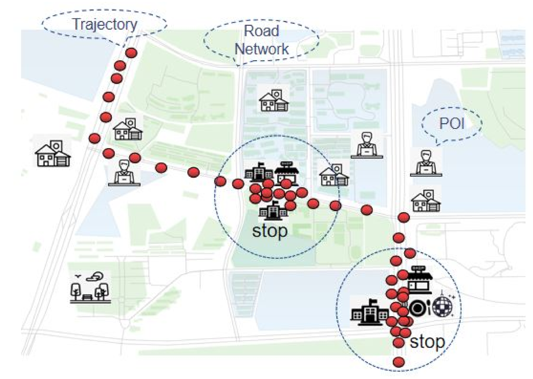
This study proposes an analytical framework for identifying stops from trajectory data. The framework seeks to measure and analyze spatio-temporal environment features surrounding the point sequence of a stop so that more accurate stop information can be obtained. Figure 2 illustrates the framework that integrates the environment information into trajectory movement. For this study, POIs and the road network structure are selected to construct stop environment context cubes according to specific business hours, which presents spatio-temporal dynamics of sequences of environmental contexts when the staying behavior occurs. A method based on the time-distance threshold is used to extract the suspected stops after reconstructing the vehicle’s trajectory data. By projecting the stop subsequences of trajectories into three-dimensional environmental context cubes, multiple characteristics of the trajectory stops could be selected and calculated, and the space-time correlation between environment context and stop sub-trajectories is further analyzed in each period. An SVM-based classifier is then employed to identify stops and predict the accuracy of the stop test dataset. Details of mobility context cube, capturing stop candidates, and stop classification will be discussed in the following sections.

3.1. Representing Dynamic Spatiotemporal Features Using Mobility Context Cube

The stopping behaviors are affected by the surrounding environmental factors. Hence the Mobility Context Cube (MCC) model is developed for presenting the surrounding environmental information dynamically and extracting appropriate features about stopping behaviors for the following SVM-based classification. This model can set the different temporal and spatial resolution to divide the surrounding space-time of stop candidates into a series of small cells. By analyzing these small cells, one can obtain crucial information (dynamic POIs and road network contexts) for the judgment of staying behaviors of moving objects. For instance, there is a restaurant POI near the candidate stop, and the occurrence time of this stop also coincides with the mealtime, and it may be a real stop. In the same way, if an entertainment POI near the candidate stops during the daytime, then this candidate stop is likely to be a false stop.

As some researchers have pointed out [54], environmental contexts are constantly changing. By that analogy, the contextual influences of the POI and road network environment may also differ in time of day. In consequence, the identification of stops may lead to erroneous conclusions when the variability of the environmental context is ignored. Additionally, the contextual impacts of the surrounding environment may also vary over time. Various types and business hours of POIs have an impact on stopping behaviors. It is clear that a majority of POIs can only offer services during their opening hours on weekdays, which affects the occurrence of staying behaviors to a varying degree. However, previous studies have largely ignored temporal variations in the POIs environment. For example, the probability of staying behavior near restaurants’ types of POIs needs more concentration during the weekdays, especially around noon and at about 7 p.m., while it appears to vary significantly over time on weekends. As a result, further research is needed to take account of the surrounding environmental factors from a dynamic spatio-temporal change perspective.

The Mobility Context Cube (MCC) connects objects and mobile environments while accurately identifying individual behaviors. It is designed to capture the complex dynamic environment and individual staying behavior. Hagerstrand T. [55] first introduced the concept of the space-time cube in the 1980s, which represents the geographic contexts of the study area (x-axis and y-axis), with three-dimension lines inside the cube representing an individual’s movement trajectories. Space-time cubes can be used for some visual analysis but have their limitations because visualization and analysis of spatio-temporal data in GIS are further complicated. In fact, GPS tracking contains dual information of time and space. If the x-axis and y-axis, respectively, describe the geographic location of the GPS points, and the z-axis represents the acquisition time of the GPS points, this stereoscopic representation method is the three-dimensional representation of the GPS trajectory. In real-world contexts, however, geographic environment contexts represented by the x-axis and y-axis are not a simple two-dimensional situation, and their influence on moving objects may change with both space and time in highly complex ways. Representation of the environmental context should thus be also extended to capture and represent the dynamic characteristics of the environment and staying behaviors by integrating the POIs’ business hours as the third dimension.

By extending the traditional space-time cube, the MCC was developed as a new analytical framework for analyzing people’s staying behavior and their dynamic relationships with their POIs environmental context. As shown in Figure 3, the MCC can be viewed as a collection of small cubes arranged on a regular grid, each of those values represents the POI context at a specific geographic location (longitude and latitude coordinates) at a specific time (POIs’ business hours). Thus, spatial and temporal variations in the POI context are rendered as the different values of the cubes in three-dimension space at various locations and times. In the time dimension of the MCC, each layer represents the POI contexts that are in business at a particular time of the day. The size of each small cube represents the temporal and spatial resolution. Different spatial and temporal resolutions of MCCs may directly be related to the dynamic expression of POIs’ spatial and temporal characteristics, thereby affecting the accuracy of recognition of staying behavior. We establish a combination of two different spatial resolutions (200 m, 100 m) and two different time resolutions (30 min, 60 min), and then compare their performance. In this way, we establish a series of MCCs to represent the POI environment around the stops.

The geographic scope of services from POIs can be assessed by creating homogeneous buffer areas covering POI locations with a specific distance (such as 200 m or 1 km). However, representation of POIs’ effects on staying behavior should take into account the effect of distance decay rather than using arbitrary distance cut-offs: environmental effects change as a function of distance, with locations farther from a factor less affected by influencing that POIs than nearer locations are, that is, it has less possibility that the staying behavior is caused by POIs. Additionally, the influence of the road network can be considered as the distance from the stop location to the nearest section, or the number of road intersections within the neighborhood of the stops.

According to the types of services and influence on moving objects, POIs in the study area were classified into 11 categories: accommodation, medical services, transport facilities, scenic spots, restaurants, financial services, educations, shopping malls, life services, entertainments, and corporate institutions. Figure 4 shows the location of these POIs at a different time of day in the study area. On the right of the picture is the POIs that influence the staying behaviors at a different period in Meixi Lake Park. Obviously, the number of POIs has changed in the same place. In addition, we discovered that POIs may have different business hours whether they are of the same type. Taking restaurants as an example, the opening hours of a Chinese restaurant are from 9 a.m. to 10 p.m., while the opening hours of KFC are 24 h a day. As a result, it is necessary to capture the POI environmental context that is in operation in different time periods in order to construct an MCC for one day. Layers of POIs would be voxelized and organized chronologically to form MCCs with a specific temporal resolution. For each time interval, based on the locations of POIs that were operated at a specific period, the surrounding POIs’ impact on staying behaviors could be analyzed. Theoretically, the higher temporal resolution provides more detailed temporal dynamics of the environmental features on any particular day.

Figure 5 shows the spatial and temporal distribution between the stops, the POIs, and road networks. The red points represent candidate stops; the yellow points symbolize all types of POI at different business hours in a day. Not only does the picture directly analyze the spatial distribution of stops in different business hours, but it also shows a visual representation of the spatial-temporal distribution of candidate stops and POIs. As mentioned above, according to two different spatial resolutions of 200 m × 200 m, 100 m × 100 m, and time resolutions of 30 min and 60 min, four MCCs were finally established. In order to conveniently analyze the spatio-temporal relationship between MCCs and stop behaviors, the geographical coordinates and time stamps of the candidate stop points in the vehicle GPS tracking are projected into MCCs. It is obvious that locations of stopping near what types of POIs at what time.

3.2. Capturing Candidate Stop Set

Once the MCCs were established, a set of sub-trajectories was extracted from raw trajectory data, and the center point of these sub-trajectories was considered to be suspected stops; it extracts sub-trajectories related to the stopping behaviors from raw trajectories. This approach sets out in detail the spatial and temporal distribution of various forms of POIs, road networks and stops during different business hours. It is a novel way for this paper to extract the stops by calculating the surrounding environmental factors.

Algorithm 1 describes the work of extracting stop candidates from raw trajectory data, where $CalculateDistance(\cdots )$ calculates the great circle distance between current GPS point $p_i$ and all points in $a\_stop$, $CalculateDuartion(\cdots )$ is computing the duration between current GPS point $p_i$ and all points in a_stop, $Merge(\cdots )$ represents the merge function that combines clusters that are continuous in time and adjacent in space. It first checks whether a sampling point $p_i$ in trajectory satisfies the predefined distance threshold ${\delta }_d$, and time threshold ${\delta }_t$ and generates the candidates set consisting of stop candidates in form of successive sampling points. In this paper, we used two empirical values to determine ${\delta }_d$ and ${\delta }_t$. We define ${\delta }_d$ as 60 m, and ${\delta }_t$ is 60 s. This method takes into account both the temporal and spatial characteristics of the staying behavior, which presents clustering characteristics according to the spatio-temporal distribution of tracking points to a certain extent.

Algorithm 1 Extracting Stops Candidates Sub-trajectories (ESCS).

Input: Trajectory T; The time threshold ${\delta }_t$; The distance threshold ${\delta }_d$

Output: Stop candidates sub-trajectories $candidates$

1:  Initialize $a\_stop$ as an empty set;

2:  Initialize $candidates$ as an empty set;

3:  for $P_{i}inT$ do    //$P_i$ is the ith point in T;

4:         $distance$ = CalculateDistance($P_i,a\_stop$);    //calculate distance between $P_i$ and all points in $a\_stop$.

5:         if $distance>{\delta }_d$ then

6:               if $a\_stop$ is an empty then

7:                       continue;

8:               else

9:                       set $a\_stop$ as an enmpty set;

10:               end if

11:         else

12:               duration = CalculateDuration($P_i,a\_stop$);

13:               if $duration\le {\delta }_t$ then

14:                     append $P_i$ to $a\_stop$;

15:               else

16:                    append $a\_stop$ to $candidates$;

17:                    set $a\_stop$ as an enmpty set;

18:               end if

19:         end if

20:  end for

21:  $candidates$ = Merge($candidates$);

22:  return $candidates$

After the time-distance threshold filtering, a merge is necessary to employ a merge to refine $candidates$. Some consecutive candidate stops sequences are very close in space. In fact, they are likely to be the same staying behavior after further inquiring about this situation. A constraint is added to merge the stops sub-trajectories that are continuous in time and adjacent in space. If the distance between two stop sub-trajectories is less than ${\delta }_d$, two stop groups should be mixed. As shown in Figure 6, there are two sub-trajectories (marked in yellow and green) contiguous both in space and time, which obviously should belong to one stopping behavior (marked in red).

In order to understand the relationship between mobility and stops more clearly, a center point from a sub-trajectories needs to be selected, which represents the stops that project into MCCs. How to choose an appropriate center point from the stops sequence? To traverse each GPS point in the stops sequence and calculate the sum of distances from that point to other points, a point in the sequence with the lowest sum of distances to all other points can be selected as the center point. Note that the center point we extracted here is the actual point in the GPS trajectory, and the real information of the trajectory is not modified.

3.3. Stop Classification Using SVM Classifier

To improve the identify precision of the real stops, this paper exploits the support vector machine classifier to distinguish staying and walking slowly to solve the problem of identifying the real stops. Unlike other classifiers, such as KNN, the decision tree, and the Ensemble algorithm, the SVM classifier has its unique advantages: low computational complexity, high prediction accuracy, efficiency, and flexibility. SVM is a supervised machine learning method, which is often used to solve classification and regression problems. The SVM-based classification, essentially, separates all the data points from the origin (in feature space) and maximizes the distance from this hyperplane to the origin (e.g., Scholkopf B. et al. [56]). The data is generally divided into two datasets: the training dataset and the test dataset. Each sample in the training set contains a “target value” (i.e., category label) and some attribute values (i.e., features or observed variables). It aims to build a model based on the training set to predict its target value by attributes of the test data.

The core idea of SVM is to use a hyperplane to divide the training data set and maximize the boundary between the two categories, and then apply the learning model of the training set to the test set to achieve classification.

A hyperplane can be defined as

$${\omega }^{T}x+b=0$$

(1)

where $\omega$ is a normal vector perpendicular to the hyperplane. For a given sample point ($x_i,y_i$), if ${\omega }^{T}x+b>0$, then $y_i=1$; if ${\omega }^{T}x+b<0$, then $y_i=-1$. $x_i$ is put into the formula, when ${\omega }^{T}x+b>0$, this can be explained as the sample point is above the hyperplane; otherwise, the sample point is below the hyperplane. In order to find the optimal decision hyperplane, the distance from any point $x_i$ is defined in the training set to the hyperplane. The formula is presented as

$$distance=\frac{|{\omega }^T{x}_i+b|}{∥\omega ∥}$$

(2)

Moreover, the point closest to the hyperplane is needed to be the farthest away from the hyperplane, which is

$$\underset{\omega ,b}{max}\frac{{min}_{x_i}({\omega }^T{x}_i+b)y_i}{∥\omega ∥}$$

(3)

but $({\omega }^T{x}_i+b)y_i>0$, ${min}_{x_i}({\omega }^T{x}_i+b)y_i$ can be defined as 1. Therefore,

$$\left\{\begin{array}{c}\underset{\omega ,b}{max}\frac{1}{\left|\omega \right|}\\ s.t.({\omega }^T{x}_i+b)\ge 1\end{array}\right.$$

(4)

By the transformation of the primal-dual relationship, the above equation can be converted to

$$\left\{\begin{array}{c}min\frac{\left|\omega \right|}{2}\\ s.t.({\omega }^T{x}_i+b)y_i-1=0\end{array}\right.$$

(5)

the optimal model can be represented as

$${\displaystyle \omega =\sum _{i=1}^n{\alpha }_i{x}_i{y}_i}$$

(6)

SVM can also use kernel functions to map feature vectors to a higher-dimensional space to reduce the complexity because of several features. The RBF kernel is usually to be the first choice when selecting the kernel function, which maps the nonlinear sample into a higher-dimensional space. Therefore, unlike the linear kernel, the RBF kernel function can deal with the nonlinear correlation between class labels and attributes. Certainly, the sigmoid kernel function also behaves similar to the RBF kernel under certain parameters. Moreover, the number of hyperparameters also affects the complexity of kernel selection, and the polynomial kernel has more hyperparameters than the RBF kernel. Generally, the RBF kernel has fewer numerical calculation difficulties. The key is that the value range from the RBF kernel is fixed. In contrast, the value of the polynomial kernel may be infinite or zero when the degree is verified large. Therefore, a RBF kernel is regarded as the most suitable function given attributes size. This kernel function is shown as follows,

$$K(x_i,x_j)=e^{\frac{{∥x_i-x_j∥}^2}{2{\delta }^2}}$$

(7)

where $∥x_i-x_j∥$ is the Euclidean distance between vectors $x_i$ and $x_j$, and $\delta$ is the Gaussian parameter.

There are two main parameters in the RBF kernel: C and Gamma. C is a penalty coefficient, namely, the tolerance for error. Gamma is a parameter that comes with RBF function when it is selected as kernel, which implicitly determines the distribution of data mapped to the new feature space. The optimal value for a given problem is unknown, so model selection (parameter search) are needed to perform to find them. A common strategy is to divide the dataset into two parts, one of which is considered unknown, the other is used to train the model. The prediction accuracy obtained from this “unknow” dataset can accurately reflect the performance of the device in classifying an independent dataset, the process of the improved version is called cross-validation. To train the classification algorithms and tune their parameters, a cross-validation and grid search are applied.

The purpose of MCC is also constructed to extract some characteristics of the surrounding environment intuitively. According to MCC with the different spatial and temporal resolution, (200 m, 60 min) is the most convenient MCC to discover features of staying behaviors. We also need to select these characteristics that can be used to describe the information of stops of GPS trajectory, and then we could distinguish between staying and walking slowly. Part of the data is selected to reflect a correlation study of the characteristics as shown in Figure 7a. For any stop behavior that occurs for any reason, the length of a stop and the speed of a stop are essential criteria for the recognition of stops. This is valid for considering the pace and length of stops according to this image. But there are still other contextual variables that need to be considered in Figure 7b. The various types of POIs, the number of road intersections and other factors have all contributed to improving the precision of the identification of stops.

For example, when only speed and stop length are considered, the Entropy is measured as 4.95, whereas the environmental contexts are added as variables, the Entropy is 1.78. It suggests that the consideration of contextual features would reduce the uncertainty of the outcome and make the extraction of stops more accurate.

As mentioned above, the staying behaviors should not only consider the characteristics of the stops themselves, for any cell of the MCC, but also the restrictive factors of the surrounding environment. Therefore, in this paper, the stop duration, the average speed, the average distance between candidate stops and 11 types of POIs, the number of 11 types of POIs, the total number of POIs, and the number of road intersections are selected as input features of SVM for stops identification (as shown in

Table 1. List of features describing the stop characteristic.

Features	Description
Stop duration	Time between the first and the last track point of a stop cluster
Average speed	Average speed between the first and the last track point of a stop cluster
The number of intersections	The number of road intersections
The number of POIs	The total number of POIs in the neighborhood of stops
The number of the different types of POIs	Different count of 11 types of POIs
Average distance from different types of POIs to stops	Average distance from the same type of POI to stops

).

To meet the computation cost raised by the massive training sample size, a GPU-accelerated LibSVM package is used to implement SVM classification. Depending on the size of the dataset and the number of attributes, we should choose the appropriate kernel function and corresponding parameters.

4. Experiment Evaluation

In this section, the proposed method is validated by experiments on real trajectory datasets. Comparative experiments between our method and five classic algorithms were conducted.

4.1. Datasets Description

In this paper, the trajectory dataset was collected by operating vehicles to perform our experiments in Yuelu District, Changsha City, Hunan Province, which is located on the north bank of the Xiang River, averaging 80m lower than sea level. The operating vehicles refer to motor vehicles that engage in profit-oriented road transportation business activities, including taxi, private large dump trucks, buses, etc. All trajectory data comes from the project in cooperation with the transportation department of Changsha City. It contains 13,661 tracks from 1 January 2015 to 7 January 2015. Each trajectory in this dataset consists of a sequence of time-stamped points. Each point contains geographical coordinate information, such as longitude and latitude. Additionally, more than 90% of these trajectories were recorded in a dense representation. As shown in

Table 2. Data description.

Dataset No.	Trjectory Amount	Sampling Rate (s)	Average Duration (h)	Average Distance (km)	Labeled Stops
1	6000	1–3	4	26	494
2	13,661	1–30	3	20	1000

, Dataset 1 covers 6000 trajectories, the sampling rate ranges from 1 to 3 s, the average duration is 4 h, and the average number of trips is approximately 26 km. Dataset 2 covers 13,661 trajectories, the sampling rate ranges from 1 to 30 s, the average duration is 3 h, and an average number of trips is approximately 20 km. Note that “Labeled stops” is the number of stops manually labeled stops in each trajectory.

In this experiment, the road network data derived from the OpenStreetMap [57] website. OpenStreetMap is a free and open source platform that provides geographic information. It allows free (or almost free) access to map images and all of our underlying map data.

Table 3. Road network data description.

Road Classification	The Length of the Road (km)	Road Network Density (km/km${}^2$)
Urban Main Roads	19.3	2.41
Seconary Roads	4063	0.58
Branch Roads	27.89	3.48

shows the basic information of road network data in Yuelu District, which have been corrected by topology revision. There are about 106 urban main roads, 729 secondary roads, and 960 branch roads.

During this work, a visual approach based on QGIS (Quantum Geographical Information System) [58] was applied to manually check and mark trajectory stops. Especially, locations that lasted longer than 30 min with high densities are carefully labeled as stops. The recorded locations are mainly used for the verification of the stop extraction algorithm. Considering that there are many short trajectory segments in this dataset, the trajectories selected for our experiment should be long enough to ensure that there are stops in the trajectories.

During the whole experiment, we collected and labeled 1000 stops, which were selected from the dataset, and covered more than 800 trajectories. These stops and relevant features are used as input elements of SVM. Additionally, all of the trajectories were urban trajectories.

Besides trajectory data and road network data, the POI data in this article come from the POI data of the Baidu Map, which can be obtained from the API provided by Baidu Map—coordinates of points of interest. Refer to the location search in the usage instructions of Baidu Maps web service API interface, we need to access the URL to request the corresponding POI data. The POI data information obtained by Baidu Map includes name, longitude and latitude coordinates, address, id, business hours, etc. This paper uses Python programming to implement the process of crawling POI data. 11 types of POIs that may be related to the occurrence of the staying behavior are considered: accommodation, medical care, transport facilities, scenic spots, restaurants, finances, educations, shopping malls, life services, entertainments, and corporate organizations. The percentage and opening hours of each type of POIs are about as shown in

Table 4. Point of Interest (POI) data description.

POI Classification	Proportion (%)	Opening Time (h)
Accommodations	15.5%	24
Medical Care	8.5%	24
Transport Facilities	16.1%	22
Scenic spots	7.8%	10
Restaurants	10.7%	22
Finances	7.7%	20
Entertainments	7.4%	24
Educations	7.8%	10
Corporate Organizations	6.9%	12
Living services	4.3%	11
Shopping Malls	7.3%	14

. Accommodations, transport facilities, and restaurants are dominant types of POIs in the study area.

4.2. Data Processing

4.2.1. Trajectory Reconstruction

It is necessary to reconstruct raw trajectory data because impacts from the buildings in the urban area and GPS devices themselves can cause outliers (as shown in Figure 8a), which will interfere with the subsequent results seriously. In this paper, a composite method of spatio-temporal filtering and Kalman filtering is used to reconstruct trajectory data. As shown in Algorithm 2, the reconstruction in this study is twofold. For each GPS point in the trajectory data, the point’s speed is estimated as the distance between the point and the next point divided by the time duration. Accordingly, the outliers in the trajectory can be removed. Figure 8b represents the reconstructed trajectory without outliers after filtering.

Algorithm 2 Trajectory Reconstruction.

Input: Trajectory T; The speed threshold v;

Output: T without outliers

1:  previous point=$P_0$;

2:  for $P_i$ in T do

3:        $v_i$=distance(previous point,$P_i$)/duration(previous point,$P_i$);

4:        if $v_i>v$ then

5:              remove $P_i$ from T;

6:        end if

7:        previous point=$P_i$;

8:  end for

9:  KalmanFilter(T)

10:  return T

Figure 9 shows the result of extracting the candidate stops in the study area. The reconstructed experimental trajectories are processed by the ESCS algorithm to obtain stop candidates’ sub-trajectories. To be noted, all sub-trajectories of candidate stops are abstracted by the center of themselves for the sake of simplicity in graphics.

4.2.2. Stops Features Extracting

After converting the stops dataset into the corresponding data format, it is also necessary to normalize these features. Attribute values of stops should be normalized by using a min-max normalization. It is very necessary to scale the data before using the SVM to train the model. The main benefit of scaling is to prevent the value range of each attribute from being too large. The span of some attribute ranges is large, while the other spans are smaller. Another benefit is that you can avoid numerical difficulties, which can be caused by large attribute values. Additionally, the experiment employed 10-fold cross-validation conducive to alleviate the model overfitting. The original dataset is randomly split into training datasets and test datasets to carry out multiple groups. In general, the ratio of the training set to the test set is set to 4:1 or 3:1. In this paper, 75% of our data is used to train the applied machine learning algorithms, and the rest is used to test their performance. After splitting the dataset into ten different subsets, we use the nine subsets to train the data and leave the last subset as test data. In the process of selecting kernel function, by comparing the performance of the combined parameters of different classifiers and kernel functions, the test result verifies that the RBF kernel function is the best. The grid.py tool and cross-validation are provided to find and adjust the best parameters C and Gamma. After running the program through Python, the optimal parameters C and Gamma can be obtained directly, and then the optimal parameters can be substituted into the original parameter model. The return value is the average classification accuracy under cross-validation. The test result reveals that the optimal parameters indeed can improve the accuracy of classification.

In order to reduce computationally and improve the classification accuracy, attribute selection can be conducted and some unimportant features of stops should be filtered. Six methods can be compared: correlation coefficient method, chi-square test method, feature selection method based on penalty term, feature selection method based on tree model, principal component analysis (PCA) method, and Linear discriminant analysis (LDA) method, and found that the corresponding classification accuracy is shown in

Table 5. The accuracy of methods for selecting attributes.

Methods	Accuracy
Correlation coefficient method	59%
Chi-square test method	67%
Feature selection method based on penalty term	60%
Feature selection method based on tree model	60%
Principal component analysis (PCA)	60%
Linear discriminant analysis (LDA)	69%

. In reality, the classification accuracy of attribute selection has not changed significantly, so 26 original features were used for subsequent tests in this paper.

4.3. MCCs Analysis

4.3.1. MCCs Constrution

Based on the characteristics of the stops, 11 types of POIs that may be related to the occurrence of the staying behavior are considered: accommodation, medical services, transport facilities, scenic spots, restaurants, financial services, education, shopping malls, life services, entertainments, and corporate institutions. As different types of POIs have specific business hours, even if they are the same type of POI. To analyze the spatiotemporal relationship between the stops and POIs, we divided all the POI data into 24 layers with a time resolution of every hour according to the business hours of the POIs. Each layer represents a POI semantic environment for a while. Therefore, it is convenient for us to construct MCCs.

Four different combinations of MCCs with two different spatial resolutions (200 m × 200 m, 100 m × 100 m) and two different temporal resolutions (30 min, 60 min) are finally established. As shown in

Table 6. Comparison of performance of different spatial and temporal resolution.

Spatial Resolution	Temporal Resolution	Entropy	${\mathit{\chi }}^2$	p-Value
100 m × 100 m	30 min	4.080	0.001	0.98
100 m × 100 m	60 min	0.595	0.203	0.65
200 m × 200 m	30 min	1.126	1.530	0.22
200 m × 200 m	60 min	1.056	2.250	0.13

, we calculated the entropy, chi-square, and p-value with different resolution combinations. Generally speaking, the higher the entropy, the more unstable the result will be. The chi-square value is more reliable when the p-value is smaller. When the spatial resolution is constant, the entropy decreases as the temporal resolution decreases, and the reliability of result increases. When the temporal resolution is constant, the entropy decrease as the temporal resolution decreases. By comparing four MCCs with different performance, we found that the combination of spatial resolution 200 m × 200 m and temporal resolution 60 min is easier to capture the spatial-temporal dynamic changes in the semantic environment of POIs.

4.3.2. Results and Analysis

Figure 10 shows the characteristics of the vehicle staying behavior in the experimental area from an MCC. According to different business hours of POIs, each layer of MCCs represents the POI semantic environment within an hour. Then, by projecting the stop points into the MCCs we constructed, staying behaviors can be able to analyze when it is more likely to occur and where the type of POIs is more likely to occur. The blue line indicates the number that the staying behaviors occurred at different moments, while the red line represents the number of ongoing staying behaviors. The continuous staying behaviors shown in red line b can better reflect people’s stopping activities. A large majority of stops of operating vehicles is mainly concentrated on the 5 periods of time: 7:00–8:00, 11:00–12:00, 13:00–14:00, 17:00–18:00, and 23:00–24:00. There are the fewest stops between 14:00 and 15:00.

The major characteristics of these operating vehicles in the experimental area include four factors: large outline size, high operating intensity, long-running time, and long vehicle age. According to the operating time and characteristics of operating vehicles, these periods of time that staying behaviors occur are in line with people’s daily habits. The two periods of 7:00–8:00 and 17:00–18:00 are the rush hours of commuting, and there are more staying behaviors. The number of stops increases, between 13:00 and 14:00, as more operating vehicles changed shifts or took short breaks at this time. From 23:00 to 24:00 is normally the time for people to sleep, and most operating vehicles have been closed. As a result, some vehicles stay in fixed parking spaces.

In other periods, the number of staying behaviors fluctuates because the types of vehicles are operating in different operating periods. There are still a lot of ongoing staying behaviors during certain times, although the number of new stops decreases. From 0:00 to 1:00, as for operating vehicles, there are still some operating trucks or buses working at night, carrying goods and passengers. During the periods 8:00–9:00 and 14:00–15:00, some operating vehicles, such as buses and taxis, served during working hours; therefore, the number of stops reduced compared to 7:00–8:00 and 13:00–14:00. From 12:00 to 13:00, the number of stops reduced due to the different mealtime of these drivers.

Figure 11 presents the types and quantities of POIs within 200 m near the stops at different periods. From this picture, the periods when the stop points are mainly concentrated are represented. For example, from 0:00 to 1:00 am, the most common places near the stop points are the POIs types of accommodation, which indicates that people may take a rest at places such as hotels and inns. From 7:00 to 8:00, the stop points are mainly focused on the types of accommodation, transport facilities, medical services, and educations, which are also the peak time for people to go to work and school in daily life. In fact, the stops in these places conform to people’s living habits. Between 17:00 and 19:00, operating vehicles at this time tend to stay at the POIs types of accommodation, catering, and company, and shows that people in the rush hours, usually return home from work locations, eating out, go shopping, etc., so they stay in these places. Between 23:00 and 24:00, the staying behaviors of operating vehicles is more likely to occur in the POIs of accommodation, medical service and financial service, which also indicates that some people who return home too late or that some of them choose to stay in hotels during this period.

4.4. Effectiveness Evaluation

In order to verify the feasibility of our method, we compared it with other stop points detection algorithms using the same data set, including the DBSCAN algorithm and method based on the time–distance threshold. In this article, we used precision, recall, and F1-Score as evaluation criteria to verify our method. The precision rate is the proportion of the sample predicted to be the stop points. The recall rate represents the percentage of true stop points predicted to be correct in all samples. F1-Score is the weighted harmonic mean of precision and recall. Their values range from 0 to 1. The higher the value, the better the experimental effect is. The computation of these values are as follows.

$$Precision=\frac{thenumberoftruestopsfound}{thenumberofstopsfound}$$

(8)

$$Recall=\frac{thenumberoftruestopsfound}{thenumberoftruestops}$$

(9)

$$F1-Score=\frac{2\times Precision\times Recall}{Precision+Recall}$$

(10)

Table 7. The accuracy of methods for selecting attributes.

Methods	Precision	Recall	F1-Score
This paper	0.78	0.90	0.83
DBSCAN	0.73	0.64	0.68
Time-Distance Threshold	0.59	0.99	0.74
CB-SMoT	0.59	0.62	0.60
DJ-Cluster	0.80	0.83	0.81
Time-Based	0.74	0.82	0.78

shows the result of the different algorithm. From the perspective of precision, compared with the other five methods, the precision of our method is slightly improved. In terms of recall, our method and the method based on the time–distance threshold are over 0.9, which is significantly larger than the DBSCAN algorithm. In terms of F1-score, which is the result of a weighted reconciliation of precision and recall, and our method is more valuable. As for the DBSCAN algorithm, although its precision is high, its main shortcoming is that it only considers regions with high spatial density; as for the method based on the time–distance threshold, its recall is high, but the precision is low. It indicates that it has a high rate of false positives and it is easy to identify the error of non-stop point as stops. For example, near an intersection, it is easier to mistake slow traffic for stops. In general, the effect of our method is better than the other five methods on the real trajectory dataset. Besides, in this study, the precision of the CB-SMoT algorithm is very low. The main reason for this is that the CB-SMoT algorithm fails to deal with fake stops. Some moving objects with a lower velocity like passing crossroads may be recognized as stops. The DJ-Cluster algorithm is an improvement based on the DBSCAN method, but it still does not consider temporal information. The time-based clustering method is time-dependent, and it is vulnerable to the time threshold. In this paper, our method considered more dynamical contextual information near stops such as POIs and road networks, it is more accurate to distinguish true stops and walking slowly, in order to reduce the rate of misjudgment. Therefore, our method worked better than the other five algorithms in a real-world trajectory.

It can be seen that certain features of the spatial setting of the stops, such as the number of different types of POIs around the stops, the average distance between the different types of POIs and the intersections, can be used to differentiate the stops to a certain degree. According to our study, the greater the number of POIs at stops, the greater the likelihood of stops at rush hour, particularly for POIs of accommodation, transport facilities and catering. In addition, the number of intersections is comparatively high, as running vehicles are more likely to have their residual behaviors under the circumstances.

5. Discussion

In this section, we first discuss what the surrounding environmental features must be used, then discuss the interaction between trajectory data and the surrounding environmental contexts to analyze the spatio-temporal semantic information of trajectory.

5.1. Which Surrounding Contextual Features Should Be Selected?

Moving objects are not isolated. They are subject to the constraints of the spatio-temporal surrounding contexts. Mining trajectory data should no longer focus on trajectories only but should also utilize rich contexts from other data sources to provide a semantic understanding of trajectories. We need to understand how trajectories are associated with or affected by the surrounding contexts. The increasing availability of contextual information (e.g., POI data, road network, and weather) can potentially create possibilities for integrating trajectory data and the surrounding contexts [13].

What we need are factors that will influence the occurrence of staying behavior. Generally speaking, the selection of features should consider two aspects. On the one hand, whether the features are divergent. On the other hand, the correlation between features and goals. The features with high relevance to the staying behaviors of moving objects should be selected preferentially. What we need are factors that will influence the occurrence of staying behavior. The observed stops are impacted by many factors simultaneously, such as the average speed, duration, local events, traffic jams, and weather. There are still numerous features that affect stops required to be extracted. This paper considers the average speed, duration, the number of intersections, the number of POIs, business hours of POIs, the types of POIs, and the distance to the POIs. Gong L. et al. [50] selected and utilized three attributes as input features of support vector machines (SVMs): stop duration, the mean distance of GPS points to the cluster centroid, and the shorter of the distances from the current location to home and the workplace. Besides, representation of POIs’ effects on staying behavior should be considered the effect of distance decay rather than using arbitrary distance cut-offs: environmental effects change as a function of distance, with locations farther from a factor less affected by influencing that POIs than nearer locations are, that is, it has less possibility that POIs cause the staying behavior. The urban road network is then divided into expressways, primary roads, secondary roads, and branch roads. The urban road network is hierarchical. The traffic flow and the distance to the different road levels are different, so the impact on vehicles’ staying behaviors is not the same. Additionally, various machine learning algorithms can be chosen to compare performance, such as ANN, random forest, and clustering. These may be some potential future research topics.

5.2. The Interaction between Trajectory Data and the Surrounding Environmental Contexts

The surrounding contextual information has uncertainty, and it is continuously changing. As there are many surrounding contexts near a location, it is ambiguous, which correlates with the trajectory. The spatio-temporal environment should be dynamically expressed. The traditional method is embodied by spatio-temporal slicing. This paper constructs MCCs to model and analyze the relationship between human behaviors and the surrounding contexts. Taking the surrounding environmental contexts into consideration will improve the accuracy of recognizing staying behaviors. Some studies discuss the interaction between trajectory data and the surrounding environmental contexts to analyze the trajectory’s spatio-temporal semantic information. It is one of the future directions of trajectory data mining. The authors of [59,60] detected the stops as the parts of a trajectory where the user stopped to perform an activity and match these stops to the possible visited POIs. The work in [61] shows that different types of POIs have different attractiveness, and the probability of staying behavior near catering POIs is relatively high. Indeed, the semantic information of the surrounding environment contexts is different between weekdays and weekends. The surrounding environmental contexts include the geographic environment and some spatial and temporal information exposed to online social media. Reference [62] infer an individual’s trip purposes by combining the knowledge from heterogeneous data sources, including trajectories, POIs, and geotagged tweets.

6. Conclusions

In this paper, a novel method is proposed to extract the stops in the individual trajectory by using the context of the dynamic surrounding environment. First, the candidate stops are extracted based on the traditional time–distance threshold method. Then, combining with the surrounding environment elements, the Mobility context cube (MCC) is constructed to analyze the relationship between the stops and POIs, and then the spatial-temporal characteristics related to the stops are selected and calculated. According to these characteristics, the SVM classifier is used to train, predict, and evaluate the accuracy of recognizing stops. Some experiments were performed to verify the algorithm’s performance, and the results demonstrate the feasibility of the proposed approach. Obviously, our approach takes full account of the complex changes in the environmental background around the stop points and more mining and analyzes the spatial and temporal characteristics of the stop points, in order to increase the accuracy of the stops. This approach of using MCC to examine the mobility background of stops from a three-dimensional space-time perspective and to classify stops through machine learning has a good impact.

The method presented in this paper can be further improved. The proposed method in this paper lacked the differences of POIs’ business hours between working days and on weekends. Second, the spectrum of service impacts of POIs can be modified at a distance, but this article does not recognize the various effects of different distance attenuation. In addition, the layout of the urban road network is hierarchical, and this paper clearly considers the effect of the number of intersections when selecting the spatial and temporal features of the stops. Certainly, the accuracy of different machine learning algorithms to extract the stops maybe different [49], these topics will be focused on in future researches. Enhancing the interaction between trajectory data and the surrounding environmental contexts to analyze the spatio-temporal semantic information of trajectory is also one of the future trajectory data mining directions.

References

1. Wu, T.; Zeng, Z.; Qin, J.; Xiang, L.; Wan, Y. An Improved HMM-Based Approach for Planning Individual Routes Using Crowd Sourcing Spatiotemporal Data. Sensors 2020, 20, 6938. [Google Scholar] [CrossRef]
2. Massimo, D.; Ricci, F. Clustering users’ pois visit trajectories for next-poi recommendation. In Information and Communication Technologies in Tourism 2019; Springer: Cham, Switzerland, 2019; pp. 3–14. [Google Scholar]
3. Kong, X.; Xia, F.; Wang, J.; Rahim, A.; Das, S.K. Time-location-relationship combined service recommendation based on taxi trajectory data. IEEE Trans. Ind. Inform. 2017, 13, 1202–1212. [Google Scholar] [CrossRef]
4. Zhang, S.; Mao, X.; Choo, K.K.R.; Peng, T.; Wang, G. A trajectory privacy-preserving scheme based on a dual-K mechanism for continuous location-based services. Inf. Sci. 2020, 527, 406–419. [Google Scholar] [CrossRef]
5. Zhong, Z.; Lee, E.E.; Nejad, M.; Lee, J. Influence of CAV clustering strategies on mixed traffic flow characteristics: An analysis of vehicle trajectory data. Transp. Res. Part C Emerg. Technol. 2020, 115, 102611. [Google Scholar] [CrossRef] [Green Version]
6. Wu, T.; Zhang, P.; Qin, J.; Wu, D.; Xiang, L.; Wan, Y. A Flood-Discharge-Based Spatio-Temporal Diffusion Method for Multi-Target Traffic Hotness Construction from Trajectory Data. IEEE Access 2020, 8, 225448–225462. [Google Scholar]
7. Yu, W. Discovering frequent movement paths from taxi trajectory data using spatially embedded networks and association rules. IEEE Trans. Intell. Transp. Syst. 2018, 20, 855–866. [Google Scholar] [CrossRef]
8. Yuan, H.; Chen, B.Y.; Li, Q.; Shaw, S.L.; Lam, W.H. Toward space-time buffering for spatiotemporal proximity analysis of movement data. Int. J. Geogr. Inf. Sci. 2018, 32, 1211–1246. [Google Scholar] [CrossRef]
9. McLean, D.J.; Skowron Volponi, M.A. Trajr: An R package for characterisation of animal trajectories. Ethology 2018, 124, 440–448. [Google Scholar] [CrossRef] [Green Version]
10. Sakuma, T.; Nishi, K.; Kishimoto, K.; Nakagawa, K.; Karasuyama, M.; Umezu, Y.; Kajioka, S.; Yamazaki, S.J.; Kimura, K.D.; Matsumoto, S.; et al. Efficient learning algorithm for sparse subsequence pattern-based classification and applications to comparative animal trajectory data analysis. Adv. Robot. 2019, 33, 134–152. [Google Scholar] [CrossRef]
11. Wu, T.; Qin, J.; Wan, Y. TOST: A Topological Semantic Model for GPS Trajectories Inside Road Networks. Int. J. Geo-Inf. 2019, 8, 410. [Google Scholar] [CrossRef] [Green Version]
12. Spaccapietra, S.; Parent, C.; Damiani, M.L.; de Macedo, J.A.; Porto, F.; Vangenot, C. A conceptual view on trajectories. Data Knowl. Eng. 2008, 65, 126–146. [Google Scholar] [CrossRef] [Green Version]
13. Li, Z. Semantic Understanding of Spatial Trajectories. In International Symposium on Spatial and Temporal Databases; Springer: Cham, Switzerland, 2017; pp. 398–401. [Google Scholar]
14. Zheng, Y. Trajectory Data Mining: An Overview. ACM Trans. Intell. Syst. Technol. 2015, 6, 1–41. [Google Scholar] [CrossRef]
15. Hariharan, R.; Toyama, K. Project Lachesis: Parsing and Modeling Location Histories. In Proceedings of the Geographic Information Science: Third International Conference, Adelphi, MD, USA, 20–23 October 2004. [Google Scholar]
16. Li, Q.; Zheng, Y.; Xie, X.; Chen, Y.; Liu, W.; Ma, W. Mining User Similarity Based on Location History. In Proceedings of the 16th ACM SIGSPATIAL International Conference on Advances in Geographic Information Systems, Irvine, CA, USA, 5–7 November 2008. [Google Scholar]
17. Pavan, M.; Mizzaro, S.; Scagnetto, I.; Beggiato, A. Finding Important Locations: A Feature-Based Approach. In Proceedings of the IEEE International Conference on Mobile Data Management, Pittsburgh, PA, USA, 15–18 June 2015. [Google Scholar]
18. Hou, Y.C.; Wang, P.C.; Liu, X.Q.; Teng, J.; Geo-Informatics, D.O. Algorithm Study for Stay Points Recognition of Spatial Trajectory Based on Velocity. Geogr. Geo-Inf. Sci. 2016, 6, 11. [Google Scholar]
19. Ankerst, M.; Breunig, M.M.; Kriegel, H.P.; Sander, J. OPTICS: Ordering Points to Identify the Clustering Structure. In Proceedings of the ACM SIGMOD International Conference on Management of Data, Philadelphia, PA, USA, 1–3 June 1999. [Google Scholar]
20. Ashbrook, D.; Starner, T. Using GPS to learn significant locations and predict movement across multiple users. Pers. Ubiquitous Comput. 2003, 7, 275–286. [Google Scholar] [CrossRef]
21. Ester, M.; Kriegel, H.; Sander, J.; Xu, X. A Density-Based Algorithm for Discovering Clusters in Large Spatial Databases with Noise. In Proceedings of the KDD 96, The Second International Conference on Knowledge Discovery and Data Mining, Portland, OR, USA, 2–4 August 1996. [Google Scholar]
22. Zhou, C.; Dan, F.; Ludford, P.; Shekhar, S.; Terveen, L. Discovering personally meaningful places. ACM Trans. Inf. Syst. 2007, 25, 12-es. [Google Scholar] [CrossRef]
23. Luo, T.; Zheng, X.; Xu, G.; Fu, K.; Ren, W. An Improved DBSCAN Algorithm to Detect Stops in Individual Trajectories. ISPRS Int. J. Geo Inf. 2017, 6, 63. [Google Scholar] [CrossRef]
24. Alvares, L.O.; Bogorny, V.; Kuijpers, B.; de Macêdo, J.A.F.; Vaisman, A.A. A model for enriching trajectories with semantic geographical information. In Proceedings of the 15th ACM International Symposium on Geographic Information Systems, Seattle, WA, USA, 7–9 November 2007. [Google Scholar]
25. Palma, A.T.; Bogorny, V.; Kuijpers, B.; Alvares, L.O. A clustering-based approach for discovering interesting places in trajectories. In Proceedings of the ACM Symposium on Applied Computing (SAC08), Fortaleza, Brazil, 16–20 March 2008. [Google Scholar]
26. Nanni, M.; Pedreschi, D. Time-focused clustering of trajectories of moving objects. J. Intell. Inf. Syst. 2006, 27, 267–289. [Google Scholar] [CrossRef]
27. Fu, Z.; Tian, Z.; Xu, Y.; Qiao, C. A Two-Step Clustering Approach to Extract Locations from Individual GPS Trajectory Data. ISPRS Int. J. Geo-Inf. 2016, 5, 166. [Google Scholar] [CrossRef]
28. Xiang, L.; Gao, M.; Wu, T. Extracting Stops from Noisy Trajectories: A Sequence Oriented Clustering Approach. ISPRS Int. J. Geo-Inf. 2016, 5, 29. [Google Scholar] [CrossRef] [Green Version]
29. Hachem, F.; Damiani, M.L. Periodic Stops Discovery through Density-Based Trajectory Segmentation. In Proceedings of the 26th ACM SIGSPATIAL International Conference on Advances in Geographic Information Systems, Seattle, WA, USA, 6–9 November 2018; pp. 584–587. [Google Scholar]
30. Hwang, S.; Vandemark, C.; Dhatt, N.; Yalla, S.V.; Crews, R.T. Segmenting human trajectory data by movement states while addressing signal loss and signal noise. Int. J. Geogr. Inf. Sci. 2018, 32, 1391–1412. [Google Scholar] [CrossRef] [Green Version]
31. Zhao, P.; Qin, K.; Ye, X.; Wang, Y.; Chen, Y. A trajectory clustering approach based on decision graph and data field for detecting hotpots. Int. J. Geogr. Inf. Sci. 2017, 31, 1101–1127. [Google Scholar]
32. Nurmi, P.; Bhattacharya, S. Identifying Meaningful Places: The Non-parametric Way. In Proceedings of the International Conference on Pervasive Computing, Sydney, Australia, 19–22 May 2008. [Google Scholar]
33. Zhang, K.; Li, H.; Torkkola, K.; Gardner, M. Adaptive Learning of Semantic Locations and Routes. In Proceedings of the International Conference on Location-and Context-Awareness, Oberpfaffenhofen, Germany, 20–21 September 2007. [Google Scholar]
34. Bermingham, L.; Lee, I. Mining place-matching patterns from spatio-temporal trajectories using complex real-world places. Expert Syst. Appl. 2019, 122, 334–350. [Google Scholar] [CrossRef]
35. Wan, C.; Zhu, Y.; Yu, J.; Shen, Y. SMOPAT: Mining semantic mobility patterns from trajectories of private vehicles. Inf. Sci. 2018, 429, 12–25. [Google Scholar] [CrossRef]
36. Taghavi, M.; Irannezhad, E.; Prato, C.G. Identifying Truck Stops from a Large Stream of GPS Data via a Hidden Markov Chain Model. In Proceedings of the IEEE Intelligent Transportation Systems Conference (ITSC2019), Auckland, New Zealand, 27–30 October 2019; pp. 2265–2271. [Google Scholar]
37. Guo, S.; Li, X.; Ching, W.; Dan, R.; Li, W.K.; Zhang, Z. GPS trajectory data segmentation based on probabilistic logic. Int. J. Approx. Reason. 2018, 103, 227–247. [Google Scholar] [CrossRef]
38. Milaghardan, A.H.; Abbaspour, R.A.; Claramunt, C. A Dempster-Shafer based approach to the detection of trajectory stop points. Comput. Environ. Urban Syst. 2018, 70, 189–196. [Google Scholar] [CrossRef] [Green Version]
39. Mura, M.C.R.; Guterres, M.X.; Oliveira, M.W.D.; Szenczuk, J.B.T.; Souza, W.S.S. Characterizing the Brazilian airspace structure and air traffic performance via trajectory data analytics. J. Air Transp. Manag. 2020, 85, 101798. [Google Scholar] [CrossRef]
40. Feng, J.; Wang, X.; Lv, H. Non-motor vehicle illegal behavior discrimination and license plate detection based on real-time video. J. Phys. Conf. Ser. 2020, 1544, 012105. [Google Scholar] [CrossRef]
41. Wang, J.; Kwan, M.; Chai, Y. An innovative context-based crystal-growth activity space method for environmental exposure assessment: A study using GIS and GPS trajectory data collected in Chicago. Int. J. Environ. Res. Public Health 2018, 15, 703. [Google Scholar] [CrossRef] [Green Version]
42. Wang, J.; Kwan, M.P. An analytical framework for integrating the spatiotemporal dynamics of environmental context and individual mobility in exposure assessment: A study on the relationship between food environment exposures and body weight. Int. J. Environ. Res. Public Health 2018, 15, 2022. [Google Scholar] [CrossRef] [Green Version]
43. Andrienko, G.L.; Andrienko, N.V. Extracting Patterns of Individual Movement Behaviour from a Massive Collection of Tracked Positions. In Proceedings of the Workshop on Behaviour Monitoring and Interpretation, Osnabrück, Germany, 10 September 2007. [Google Scholar]
44. Cao, X.; Cong, G.; Jensen, C.S. Mining Significant semantic Locations from Data. In Proceedings of the 36th International Conference on Vary Large Data Bases (VLDB), Singapore, 13–17 September 2010; Volume 3. [Google Scholar]
45. Spinsanti, L.; Ostermann, F.O. Automated geographic context analysis for volunteered information. Appl. Geogr. 2013, 43, 36–44. [Google Scholar] [CrossRef]
46. Yan, Z.; Chakraborty, D.J.; Parent, C.; Spaccapietra, S.; Aberer, K. Semantic Trajectories: Mobility Data Computation and Annotation. ACM Trans. Intell. Syst. Technol. 2013, 4, 1–38. [Google Scholar] [CrossRef]
47. Dandrea, A.; Cappadona, C.; La Rosa, G.; Pellegrino, O. A functional road classification with data mining techniques. Transport 2014, 29, 419–430. [Google Scholar] [CrossRef] [Green Version]
48. Lv, M.; Chen, L.; Xu, Z.; Li, Y.; Chen, G. The discovery of personally semantic places based on trajectory data mining. Neurocomputing 2016, 173, 1142–1153. [Google Scholar] [CrossRef]
49. Rehrl, K.; Gröchenig, S.; Kranzinger, S. Why did a vehicle stop? A methodology for detection and classification of stops in vehicle trajectories. Int. J. Geogr. Inf. Sci. 2020, 34, 1953–1979. [Google Scholar] [CrossRef]
50. Gong, L.; Sato, H.; Yamamoto, T.; Miwa, T.; Morikawa, T. Identification of activity stop locations in GPS trajectories by density-based clustering method combined with support vector machines. J. Mod. Transp. 2015, 23, 202–213. [Google Scholar] [CrossRef] [Green Version]
51. Gong, L.; Yamamoto, T.; Morikawa, T. Identification of activity stop locations in GPS trajectories by DBSCAN-TE method combined with support vector machines. Transp. Res. Procedia 2018, 32, 146–154. [Google Scholar] [CrossRef]
52. Schneider, C.; Grochenig, S.; Venek, V.; Leitner, M.; Reich, S. A Framework for Evaluating Stay Detection Approaches. ISPRS Int. J. Geo-Inf. 2017, 6, 315. [Google Scholar] [CrossRef] [Green Version]
53. Van Dijk, J. Identifying activity-travel points from GPS-data with multiple moving windows. Comput. Environ. Urban Syst. 2018, 70, 84–101. [Google Scholar] [CrossRef]
54. Kwan, M. The Uncertain Geographic Context Problem. Ann. Assoc. Am. Geogr. 2012, 102, 958–968. [Google Scholar] [CrossRef]
55. Hagerstrand, T. What about People in Regional Science? Pap. Reg. Sci. 1970, 24, 7–24. [Google Scholar] [CrossRef]
56. Scholkopf, B.; Williamson, R.C.; Smola, A.J.; Shawetaylor, J.; Platt, J. Support Vector Method for Novelty Detection. In Proceedings of the Neural Information Processing Systems (NIPS), Denvor, CO, USA, 1 January 2000; pp. 582–588. [Google Scholar]
57. OpenStreetMap. 2020. Available online: https://www.openstreetmap.org/ (accessed on 20 May 2020).
58. QGIS. 2020. Available online: https://www.qgis.org/en/site/ (accessed on 20 May 2020).
59. Furletti, B.; Cintia, P.; Renso, C.; Spinsanti, L. Inferring human activities from GPS tracks. In Proceedings of the ACM SIGKDD International Workshop on Urban (UrbComp 2013), Chicago, IL, USA, 11 August 2013. [Google Scholar]
60. Chen, C.; Jiao, S.; Zhang, S.; Liu, W.; Feng, L.; Wang, Y. TripImputor: Real-Time Imputing Taxi Trip Purpose Leveraging Multi-Sourced Urban Data. IEEE Trans. Intell. Transp. Syst. 2018, 19, 3292–3304. [Google Scholar] [CrossRef]
61. Gong, L.; Liu, X.; Wu, L.; Liu, Y. Inferring trip purposes and uncovering travel patterns from taxi trajectory data. Cartogr. Geogr. Inf. Sci. 2016, 43, 103–114. [Google Scholar] [CrossRef]
62. Meng, C.; Cui, Y.; He, Q.; Su, L.; Gao, J. Travel purpose inference with GPS trajectories, POIs, and geo-tagged social media data. In Proceedings of the 2017 IEEE International Conference on Big Data, Boston, MA, USA, 11–14 December 2017. [Google Scholar]
Figure 1. The example of stops in individual trajectory.
Sustainability 13 00690 g001
Figure 2. The proposed analytical framework.
Sustainability 13 00690 g002
Figure 3. Implementation of mobility context cube.
Sustainability 13 00690 g003
Figure 4. The mobility context layers in different time of a day in Yuelu District.
Sustainability 13 00690 g004
Figure 5. The spatial and temporal distribution between stops and POIs. The red dots represent candidate stops; the green dots symbolize all types of POI at different business hours in a day.
Sustainability 13 00690 g005
Figure 6. An example of stop sequences being merged.
Sustainability 13 00690 g006
Figure 7. Some features to be considered.
Sustainability 13 00690 g007
Figure 8. An example of signal loss in an individual trajectory.
Sustainability 13 00690 g008
Figure 9. The result of extracting candidate stops.
Sustainability 13 00690 g009
Figure 10. The number of stops in different time zones.
Sustainability 13 00690 g010
Figure 11. The number of stops for different POI types during different business hours.
Sustainability 13 00690 g011