Science, Technology and Innovation Policy Indicators and Comparisons of Countries through a Hybrid Model of Data Mining and MCDM Methods


Abstract
:1. Introduction
2. Methodology and Data
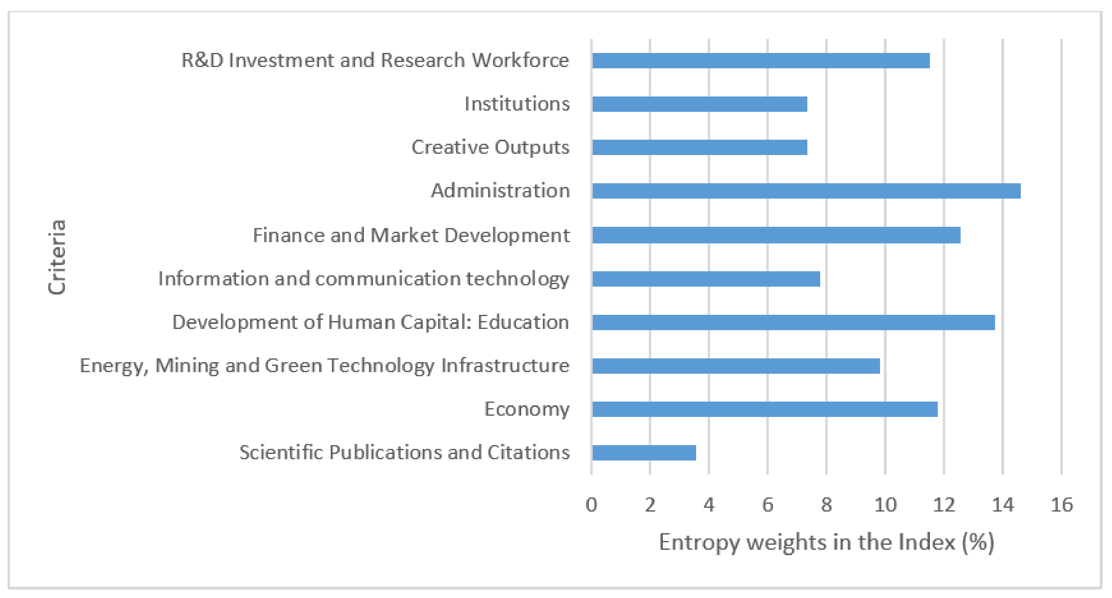
2.1. Shannon Entropy and Objective Weights
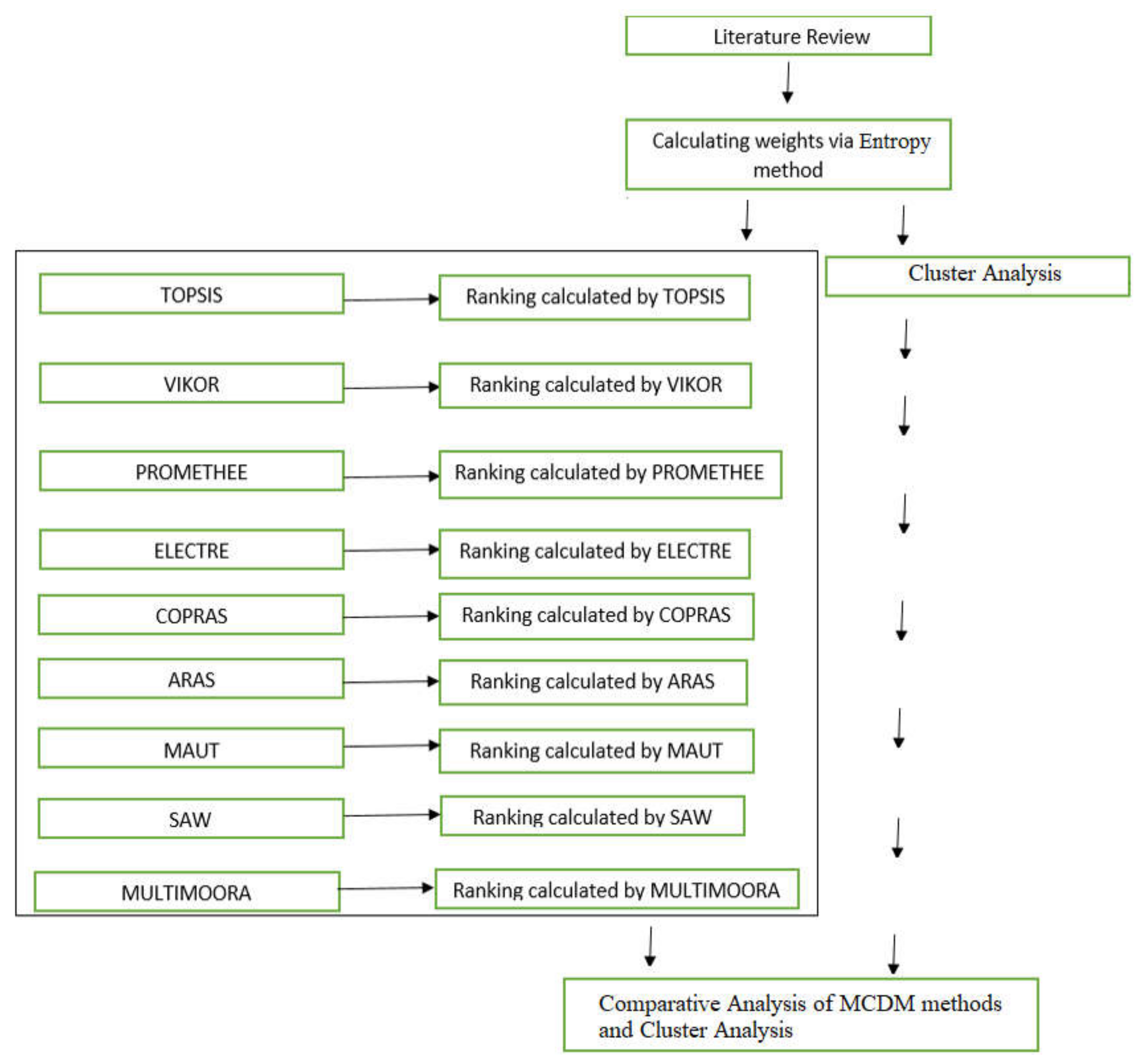
2.2. Ranking of Countries Based on MCDM Methods
2.2.1. TOPSIS (Technique for Order Preference by Similarity to Ideal Solution) Method
2.2.2. VIKOR (Vise Kriterijumska Optimizacija I Kompromisno Resenje) Multi-Criteria Optimization and Compromise Solution Method
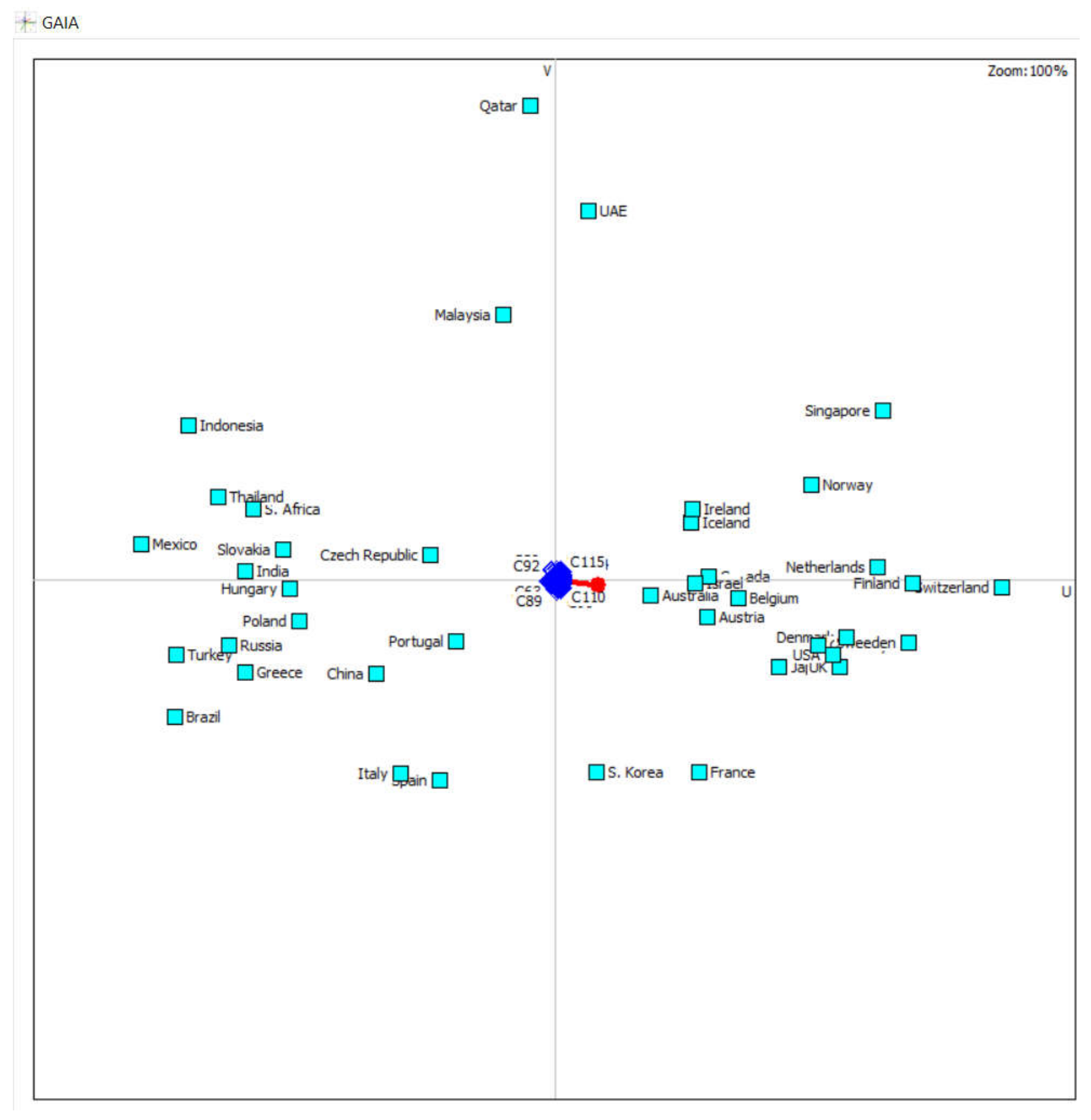
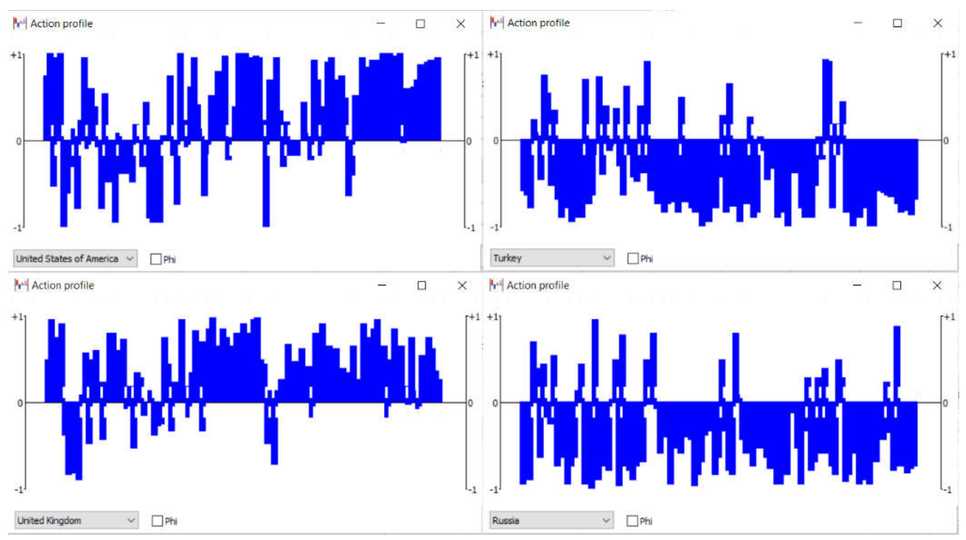
2.2.3. PROMETHEE
2.2.4. ELECTRE (Elimination and Choice Translating Reality English) Method
2.2.5. COPRAS (Complex Proportional Assesment) Method
2.2.6. ARAS (A New Additive Ratio Assessment) Method
2.2.7. Multimoora (The Multi-Objective Optimization by Ratio Analysis) Method
2.2.8. SAW (Simple Additive Weighting) Method
2.2.9. MAUT (Multi-Attribute Utility Theory) Method
- The largest value of the relevant criterion.
- : The smallest value of the relevant criterion.
- Current value of the cell under calculation.
- U(x): Benefit value of the relevant alternative.
- ui(xi): The utility value of the alternative in terms of the relevant criteria.
- Wi: weight value of the relevant criterion.
2.3. K-Means Clustering Algorithm
- (1)
- Initialize K centre locations (c1, ..., cK).
- (2)
- Assign each xi to its nearest cluster centre ck.
- (3)
- Update each cluster centre ck as the mean of all xi that have been assigned as closest to it.
- (4)
- Calculate .
- (5)
- If the value of D has converged, then return (c1,..., cK); else go to Step 2.
3. Results
4. Discussion
5. Conclusions
Author Contributions
Funding
Institutional Review Board Statement
Informed Consent Statement
Data Availability Statement
Conflicts of Interest
Appendix A

| No. | Indicator | Description | Criteria/Dimension | Source |
|---|---|---|---|---|
| 1 | Citations per publication | Number of citations per publication | Scientific Publications and Citations | Scimago (2019) |
| 2 | The productivity and citation impact of the publications of a scientist or scholar | H index | Scientific Publications and Citations | Scimago (2019) |
| 3 | International scientific collaboration | International Scientific Collaboration (%) | Scientific Publications and Citations | Scimago (2019) |
| 4 | Scientific and technical journal articles | Number of scientific and technical journal articles | Scientific Publications and Citations | Index Mundi, OECD, World Bank |
| 5 | The citation impact of scientific production | Number of citable documents | Scientific Publications and Citations | Scimago (2019) |
| 6 | Trade | Trade (% of GDP) | Economy | Index Mundi, OECD, World Bank |
| 7 | Agriculture, forestry, and fishing, value added | Agriculture, forestry, and fishing, value added (% of GDP) | Economy | Index Mundi, Trading Economics, World Bank |
| 8 | Services, value added | Services, value added (annual % growth) | Economy | Index Mundi, OECD, World Bank |
| 9 | Manufacturing, value added | Manufacturing, value added (annual % growth) | Economy | Index Mundi, Trading Economics |
| 10 | Industry (including construction), value added | Industry (including construction), value added (% of GDP) | Economy | OECD, World Bank |
| 11 | Medium and high-tech industry | Medium and high-tech industry (% manufacturing value added), Index Score | Economy | Index Mundi (2017), World Bank |
| 12 | Innovation | Innovation Score | Economy | The Global Competitiveness Index (2018), World Bank |
| 13 | Industrialization Intensity | Industrialization Intensity Index, Value, 0–1 (best) | Economy | The Global Competitiveness Index (2018), World Bank |
| 14 | Production process sophistication | Production process sophistication, Index Score 1–7 (best) | Economy | The Global Competitiveness Index (2018), World Bank |
| 15 | Nature of competitive advantage | Nature of competitive advantage, Index Score 1–7 (best) | Economy | The Global Competitiveness Index (2018), World Bank |
| 16 | High-technology exports minus re-exports | High-technology exports minus re-exports, Index Score | Economy | The Global Innovation Index (2019) |
| 17 | High-tech imports | High-tech imports, Index Score | Economy | The Global Innovation Index (2019) |
| 18 | Intellectual property payments | Intellectual property payments, Index Score | Economy | The Global Innovation Index (2019) |
| 19 | GDP per unit of energy use | GDP per unit of energy use, Index Score | Energy, Mining and Green Technology Infrastructure | The Global Innovation Index (2019) |
| 20 | Environmental performance, | Environmental performance, Index Score | Energy, Mining and Green Technology Infrastructure | The Global Innovation Index (2019) |
| 21 | ISO 14001 Environmental certificates | ISO 14001 Environmental certificates, Index Score | Energy, Mining and Green Technology Infrastructure | The Global Innovation Index (2019) |
| 22 | Adjusted savings: energy depletion | Adjusted savings: energy depletion (% of GNI) | Energy, Mining and Green Technology Infrastructure | Index Mundi, World Bank |
| 23 | Energy intensity level of primary energy | Energy intensity level of primary energy (MJ/$2011 PPP GDP) | Energy, Mining and Green Technology Infrastructure | Trading Economics, World Bank |
| 24 | Fossil fuel energy consumption | Fossil fuel energy consumption (% of total) | Energy, Mining and Green Technology Infrastructure | Trading Economics, World Bank |
| 25 | Renewable electricity output | Renewable electricity output (% of total electricity output) | Energy, Mining and Green Technology Infrastructure | Trading Economics, World Bank |
| 26 | Renewable energy consumption | Renewable energy consumption (% of total final energy consumption) | Energy, Mining and Green Technology Infrastructure | Trading Economics, World Bank |
| 27 | Alternative and nuclear energy | Alternative and nuclear energy (% of total energy use) | Energy, Mining and Green Technology Infrastructure | Trading Economics, World Bank |
| 28 | Ores and metals exports | Ores and metals exports (% of merchandise exports) | Energy, Mining and Green Technology Infrastructure | Trading Economics, World Bank |
| 29 | Fuel imports | Fuel imports (% of merchandise imports) | Energy, Mining and Green Technology Infrastructure | Trading Economics, World Bank |
| 30 | Energy imports | Energy imports, net (% of energy use) | Energy, Mining and Green Technology Infrastructure | Trading Economics, World Bank |
| 31 | CO2 emissions | CO2 emissions (metric tons per capita) | Energy, Mining and Green Technology Infrastructure | Trading Economics, World Bank |
| 32 | Total greenhouse gas emissions | Total greenhouse gas emissions (kt of CO2 equivalent) | Energy, Mining and Green Technology Infrastructure | Trading Economics, World Bank |
| 33 | Methane emissions | Methane emissions (kt of CO2 equivalent) | Energy, Mining and Green Technology Infrastructure | Trading Economics, World Bank |
| 34 | Nitrous oxide emissions | Nitrous oxide emissions (thousand metric tons of CO2 equivalent) | Energy, Mining and Green Technology Infrastructure | Trading Economics, World Bank |
| 35 | School life expectancy | School life expectancy, years | Human Capital Development: Education | The Global Innovation Index (2019), Trading Economics, World Bank |
| 36 | Expenditure on education | Expenditure on education, % GDP | Human Capital Development: Education | The Global Innovation Index (2019), Trading Economics, World Bank |
| 37 | Tertiary enrolment | Tertiary enrolment, % | Human Capital Development: Education | The Global Innovation Index (2019), Trading Economics, World Bank, Index Mundi |
| 38 | PISA scales in reading, maths, & science | PISA scales in reading, maths, & science, Score | Human Capital Development: Education | The Global Innovation Index (2019), International Money Fund |
| 39 | Graduates in science & engineering | Graduates in science & engineering, % | Human Capital Development: Education | The Global Innovation Index (2019) |
| 40 | QS university ranking | QS university ranking, average score | Human Capital Development: Education | The Global Competitiveness Index (2018), World Bank |
| 41 | Quality of the education system | Quality of the education system, Index Score | Human Capital Development: Education | The Global Competitiveness Index (2018), World Bank |
| 42 | Quality of math and science education | Quality of math and science education, Index Score | Human Capital Development: Education | The Global Competitiveness Index (2018), World Bank, Trends in International Mathematics and Science Study |
| 43 | Internet access in schools | Internet access in schools, Index Score | Human Capital Development: Education | The Global Competitiveness Index (2018), World Bank |
| 44 | Availability of latest technologies | Availability of latest Technologies, Index Score | Human Capital Development: Education | The Global Competitiveness Index (2018), World Bank |
| 45 | Local availability of specialized training services | Local availability of specialized training services Index Score | Human Capital Development: Education | The Global Competitiveness Index (2018) |
| 46 | Government funding/pupil, secondary | Government funding/pupil, secondary, % GDP/cap | Human Capital Development: Education | The Global Innovation Index (2019), Trading Economics, World Bank |
| 47 | Government expenditure per student, tertiary | Government expenditure per student, tertiary (% of GDP per capita) | Human Capital Development: Education | The Global Innovation Index (2019), Trading Economics, World Bank |
| 48 | Tertiary inbound mobility | Tertiary inbound mobility, % | Human Capital Development: Education | The Global Innovation Index (2019) |
| 49 | ICT access | ICT Access, Index Score | Information and Communication Technology | The Global Innovation Index (2019) |
| 50 | ICT use | ICT use, Index Score | Information and Communication Technology | The Global Innovation Index (2019) |
| 51 | ICTs & business model creation | ICTs & business model creation, Index Value | Information and Communication Technology | The Global Innovation Index (2019) |
| 52 | Laws relating to ICTs | Laws relating to ICTs, Index Score, 1–7 (best) | Information and Communication Technology | Trading Economics, World Bank |
| 53 | ICTs & organizational model creation | ICTs & organizational model creation, Index Value | Information and Communication Technology | The Global Innovation Index (2019) |
| 54 | ICT services exports | ICT services exports, Index Score | Information and Communication Technology | The Global Innovation Index (2019) |
| 55 | ICT services imports | ICT services imports, Index Score | Information and Communication Technology | The Global Innovation Index (2019) |
| 56 | The ICT Development Index (IDI) | The ICT Development Index (IDI) Score | Information and Communication Technology | International Telecommunication Union (ITU) |
| 57 | Credit | Credit Score | Finance and Market Sophistication | The Global Innovation Index (2019) |
| 58 | Investment | Investment Score | Finance and Market Sophistication | The Global Innovation Index (2019) |
| 59 | Trade, competition, & market scale | Trade, competition, & market scale, Index Score | Finance and Market Sophistication | The Global Innovation Index (2019) |
| 60 | Business environment | Business environment, Index Score | Finance and Market Sophistication | The Global Innovation Index (2019) |
| 61 | Intensity of local competition | Intensity of local competition, Index Score, 1–7 (best) | Finance and Market Sophistication | Trading Economics, World Bank |
| 62 | Extent of market | Extent of market, Index Score | Finance and Market Sophistication | The Global Competitiveness Index (2018), World Bank |
| 63 | Foreign market size | Foreign market size, Index Score | Finance and Market Sophistication | The Global Competitiveness Index (2018), World Bank |
| 64 | Labor force participation, female | Labor force participation rate, female (% of female population ages 15+) | Finance and Market Sophistication | World Bank |
| 65 | Exports of goods and services | Exports of goods and services (% of GDP) | Finance and Market Sophistication | The Global Competitiveness Index (2018), World Bank |
| 66 | GDP per capita | GDP per capita (current US$) | Finance and Market Sophistication | Trading Economics, World Bank, Index Mundi |
| 67 | Real GDP growth | Real GDP growth rate (%) | Finance and Market Sophistication | World Bank, International Money Fund (IMF) |
| 68 | Average monthly net salary | Average Monthly Net Salary (After Tax, US$) | Finance and Market Sophistication | Numbeo |
| 69 | Unemployment | Unemployment, total (% of total labor force) | Finance and Market Sophistication | International Labour Organization (ILO), World Bank |
| 70 | Efficiency of government spending | Efficiency of government spending, Index Score | Governance | The World Economic Forum (WEF) Report, The Global Competitiveness Index |
| 71 | Transparency of government policymaking | Transparency of government policymaking, Index Score, 1–7 (best) | Governance | The Global Competitiveness Index, World Bank |
| 72 | Favoritism in decisions of government officials | Favoritism in decisions of government officials, Index Score, 1–7 (best) | Governance | The Global Competitiveness Index, World Bank |
| 73 | Diversion of public funds | Diversion of public funds, Index Score 1–7 (best) | Governance | The Global Competitiveness Index, World Bank |
| 74 | Public trust in politicians | Public trust in politicians, Index Score, 1–7 (best) | Governance | The Global Competitiveness Index, World Bank |
| 75 | Judicial independence | Judicial independence, Index Score, 1–7 (best) | Governance | The Global Competitiveness Index, World Bank |
| 76 | Government Effectiveness | Government Effectiveness Score, Index Score, 2018 | Governance | The World Government Index (WGI) |
| 77 | Voice and Accountability | Voice and Accountability, Index Score, 2018 | Governance | The World Government Index (WGI) |
| 78 | Political Stability and Absence of Violence/Terrorism | Political Stability and Absence of Violence/Terrorism, Index Score, 2018 | Governance | The World Government Index (WGI) |
| 79 | Government’s online service | Government’s online service, Index Score | Governance | The Global Innovation Index (2019) |
| 80 | E-participation | E-participation, Index Score | Governance | The Global Innovation Index (2019), World Bank |
| 81 | Effectiveness of law-making bodies | Effectiveness of law-making bodies, Index Score, 1–7 (best) | Governance | World Bank |
| 82 | Political environment | Political environment, Index Score | Governance | The Global Innovation Index |
| 83 | Charges for the use of intellectual property not included elsewhere receipts | Charges for the use of intellectual property not included elsewhere receipts (% of total trade), Index Score | Governance | The Global Innovation Index |
| 84 | Charges for the use of intellectual property, payments | Charges for the use of intellectual property, payments (BoP, current US$) | Governance | Index Mundi, World Bank |
| 85 | Regulatory environment | Regulatory environment, Index Score | Governance | The Global Innovation Index |
| 86 | Patent families filed by residents | Number of patent families filed by residents in at least two offices (per billion PPP$ GDP), Index Score | Creative Outputs | The Global Innovation Index |
| 87 | Resident patent applications | Number of resident patent applications at national or regional office (per billion PPP$ GDP), Index Score | Creative Outputs | The Global Innovation Index |
| 88 | International patent applications | Number of international patent applications at the PCT (per billion PPP$ GDP), Index Score | Creative Outputs | The Global Innovation Index |
| 89 | Trademark application | Trademark application count by origin (per billion PPP$ GDP), Index Score | Creative Outputs | The Global Innovation Index |
| 90 | Industrial designs | Industrial designs by origin per billion PPP$ GDP, Index Score | Creative Outputs | The Global Innovation Index |
| 91 | High-tech and medium-high-tech output | High-tech and medium-high-tech output, Index Score | Creative Outputs | The Global Innovation Index |
| 92 | Creative goods exports | Creative goods exports, Index Score | Creative Outputs | The Global Innovation Index |
| 93 | Cultural & creative services exports | Cultural & creative services exports, Index Score | Creative Outputs | The Global Innovation Index |
| 94 | Mobile app creation | Mobile app creation, Index Score | Creative Outputs | The Global Innovation Index |
| 95 | Value chain breadth | Value chain breadth, Index Score, 1–7 (best) | Creative Outputs | The Global Competitiveness Index, World Bank |
| 96 | University-industry collaboration in R&D | University-industry collaboration in R&D, Index Score | Institutions | The Global Competitiveness Index, World Bank |
| 97 | Quality of scientific research institutions | Quality of scientific research institutions, Index Score, 1–7 (best) | Institutions | The Global Competitiveness Index, World Bank |
| 98 | Government procurement of advanced technology products | Government procurement of advanced technology products, Index Score | Institutions | The Global Competitiveness Index, World Bank |
| 99 | State of cluster development | State of cluster development, Index Score | Institutions | The Global Innovation Index, World Bank |
| 100 | Ease of access to loans | Ease of access to loans, Index Score, 1–7 (best) | Institutions | World Bank |
| 101 | Venture capital availability | Venture capital availability, Index Score, 1–7 (best) | Institutions | The Global Competitiveness Index, World Bank |
| 102 | Venture capital deals | Venture capital deals/bn PPP$ GDP, Index Score | Institutions | The Global Innovation Index |
| 103 | JV-strategic alliance deals | V-strategic alliance deals/bn PPP$ GDP, Index Score | Institutions | The Global Innovation Index |
| 104 | Average expenditure on R&D of the top three global companies | Average expenditure on R&D of the top three global companies mn US$, Index Score | Institutions | The Global Innovation Index |
| 105 | Researchers | Researchers, FTE/per million population Score | R&D Investment and Research Workforce | The Global Innovation Index |
| 106 | Gross expenditure on R&D | Gross expenditure on R&D, Score | R&D Investment and Research Workforce | The Global Innovation Index |
| 107 | Employment in knowledge-intensive services | Employment in knowledge-intensive services (% of workforce) | R&D Investment and Research Workforce | The Global Innovation Index, World Bank |
| 108 | GERD performed by business enterprise, | GERD performed by business enterprise, % GDP | R&D Investment and Research Workforce | The Global Innovation Index, World Bank |
| 109 | GERD financed by business enterprise | GERD financed by business enterprise, % | R&D Investment and Research Workforce | The Global Innovation Index, World Bank |
| 110 | Females employed with advanced degrees | Females employed with advanced degrees, % | R&D Investment and Research Workforce | The Global Innovation Index, World Bank |
| 111 | Extent of staff training | Extent of staff training, Index Score, 1–7 (best) | R&D Investment and Research Workforce | World Bank |
| 112 | Country capacity to retain talent | Country capacity to retain talent, Index Score, 1–7 (best) | R&D Investment and Research Workforce | World Bank |
| 113 | Capacity for innovation | Capacity for innovation, Index Score, 1–7 (best) | R&D Investment and Research Workforce | The Global Competitiveness Index, World Bank |
| 114 | Company spending on R&D | Company spending on R&D, Index Score, 1–7 (best) | R&D Investment and Research Workforce | The Global Competitiveness Index, World Bank |
| 115 | Availability of scientists and engineers | Availability of scientists and engineers, Index Score, 1–7 (best) | R&D Investment and Research Workforce | The Global Competitiveness Index, World Bank |
References
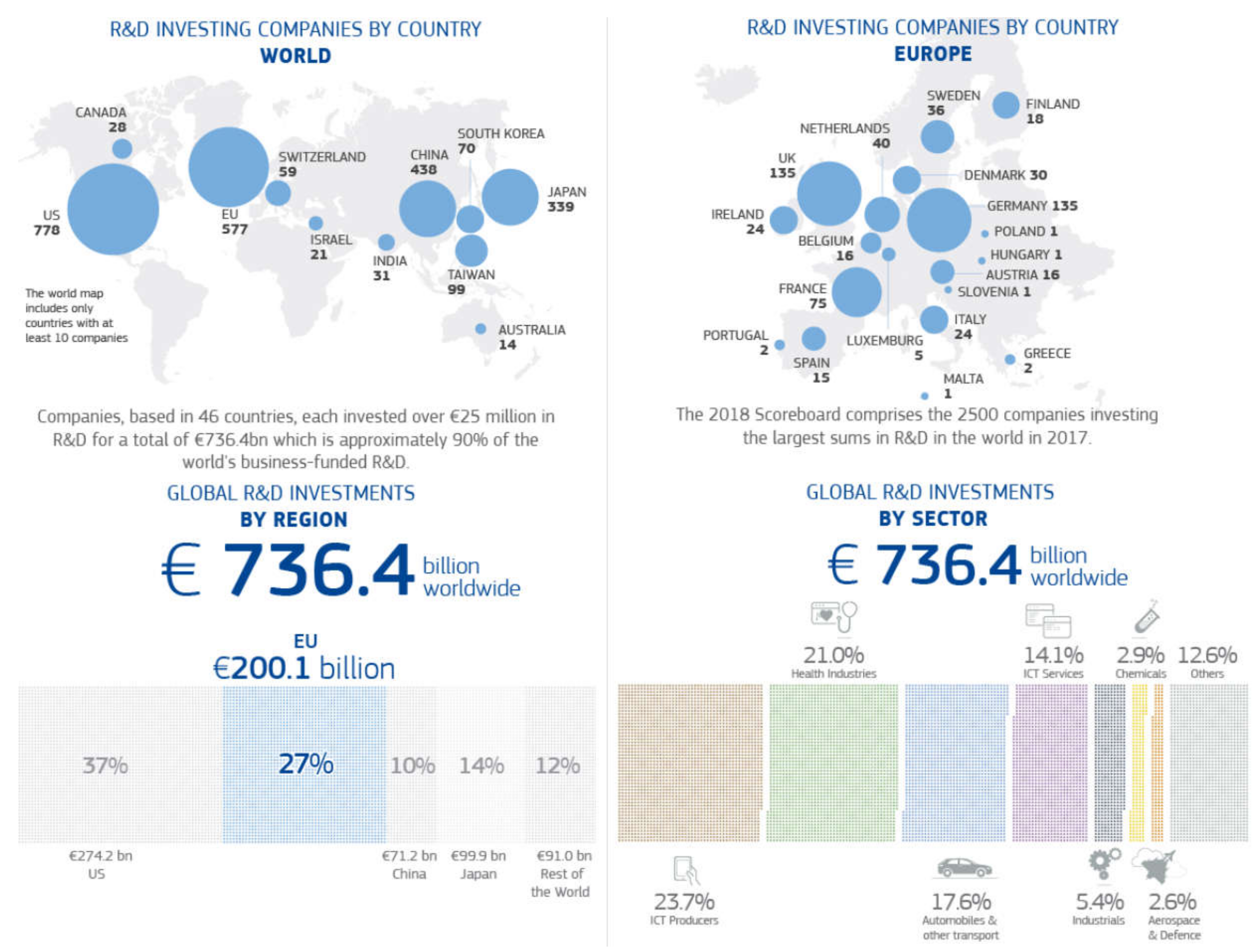
- Hernández, H.; Grassano, N.; Tübke, A.; Potters, L.; Gkotsis, P.; Vezzani, A. The 2018 EU Industrial R&D Investment Scoreboard; EUR 29450 EN; Publications Office of the European Union: Luxembourg, 2018. [Google Scholar]
- Das, A. Handbook of innovation indicators and measurement. J. Scientometr. Res. 2015, 4, 206–207. [Google Scholar]
- OECD. Oslo Manual, Guidelines for Collecting, Reporting and Using Data on Innovation; OECD Publishing: Paris, France, 2018. [Google Scholar]
- Orhan, M.; Aytekin, M. Türkiye ile AB’ye Son Katılan Ülkelerin Ar-Ge Performanslarrının CRITIC Ağırlıklı MAUT ve SAW Yöntemiyle Kıyaslanması. Bus. Manag. Stud. An Int. J. 2020, 8, 754–778. [Google Scholar] [CrossRef]
- Lin, C.K.; Shyu, J.Z.; Ding, K. A cross-strait comparison of innovation policy under industry 4.0 and sustainability development transition. Sustainability 2017, 9, 786. [Google Scholar] [CrossRef]
- Chaurasia, R.; Bhikajee, M. Adding Entrepreneurship to India’s Science, Technology & Innovation Policy. J. Technol. Manag. Innov. 2016, 11, 86–103. [Google Scholar]
- Sun, Y.; Cao, C. The dynamics of the studies of China’s science, technology and innovation (STI): A bibliometric analysis of an emerging field. Scientometrics 2020, 1–31. [Google Scholar] [CrossRef]
- Erdin, C.; Özkaya, G. ASEAN Ülkeleri ve Türkiye’nin TOPSIS Yöntemiyle Sürdürülebilir Gelişmişlik Endeksi Çerçevesinde Performans Değerlendirmesi. Yıldız Sosyal Bilimler Enstitüsü Dergisi 2017, 1, 150–163. [Google Scholar]
- Salam, S.; Hafeez, M.; Mahmood, M.T.; Iqbal, K.; Akbar, K. The dynamic relation between technology adoption, technology innovation, human capital and economy: Comparison of lower-middle-income countries. Interdiscip. Descr. Complex Syst. INDECS 2019, 17, 146–161. [Google Scholar] [CrossRef]
- Blažek, J.; Kadlec, V. Knowledge bases, R&D structure and socio-economic and innovation performance of European regions. Innov. Eur. J. Soc. Sci. Res. 2019, 32, 26–47. [Google Scholar]
- Canbolat, Y.B.; Chelst, K.; Garg, N. Combining decision tree and MAUT for selecting a country for a global manufacturing facility. Omega 2007, 35, 312–325. [Google Scholar] [CrossRef]
- Kang, D.; Jang, W.; Kim, Y.; Jeon, J. Comparing national innovation system among the USA, Japan, and Finland to improve Korean deliberation organization for national science and technology policy. J. Open Innov. Technol. Market Complex 2019, 5, 82. [Google Scholar] [CrossRef] [Green Version]
- Manyuchi, A.E. Conceptualizing and institutions facilitating ‘use’of innovation indicators in South Africa’s science, technology and innovation policymaking. Afr. J. Sci. Technol. Innov. Dev. 2018, 10, 483–492. [Google Scholar] [CrossRef]
- Özbek, A.; Demirkol, İ. Avrupa Birliği Ülkeleri İle Türkiye’nin Ekonomik Göstergelerinin Karşılaştırılması. J. Manag. Econ. 2019, 26. [Google Scholar] [CrossRef]
- SCImago. SJR-SCImago Journal & Country Rank. Available online: https://www.scimagojr.com/countryrank.php (accessed on 6 April 2020).
- Indexmundi. Country Facts. Available online: https://www.indexmundi.com/ (accessed on 5 April 2020).
- OECD; S.R. Group. Compendium of Bibliometric Science Indicators; OECD: Paris, France, 2016. [Google Scholar]
- Unesco, U.I.S. Science, Technology and Innovation. Available online: http://data.uis.unesco.org/Index.aspx (accessed on 3 April 2020).
- World Bank. Indicators. Available online: https://data.worldbank.org/indicator?tab=all (accessed on 10 March 2020).
- TradingEconomics. Trading Economics. Available online: https://tradingeconomics.com/ (accessed on 15 April 2020).
- Schwab, K. The Global Competitiveness Report 2019; WEF: Lausanne, Switzerland, 2019. [Google Scholar]
- Dutta, S.; Lanvin, B.; Wunsch-Vincent, S. The Global Innovation Index 2019: Creating Healthy Lives—The Future of Medical Innovation; Cornell University, INSEAD, and WIPO: New York, NY, USA, 2019. [Google Scholar]
- ITU. The ICT Development Index (IDI): Conceptual Framework and Methodology. 2017. Available online: https://www.itu.int/net4/ITU-D/idi/2017/index.html (accessed on 18 February 2020).
- IMF. International Monetary Fund. Fiscal Monitor Reports 2019. Available online: https://www.imf.org/en/Publications/FM (accessed on 11 March 2020).
- ILO. ILOSTAT Database. 2019. Available online: https://ilostat.ilo.org/data/ (accessed on 13 February 2020).
- Numbeo. Quality of Life Index for Country. 2020. Available online: https://www.numbeo.com/quality-of-life/rankings_by_country.jsp (accessed on 9 February 2020).
- Brauers, W.K.M.; Zavadskas, E.K. Robustness of MULTIMOORA: A method for multi-objective optimization. Informatica 2012, 23, 1–25. [Google Scholar] [CrossRef]
- Kahraman, Ç.; Abdulhamit, E.; Özevin, O. Futbol Takımlarının Finansal Ve Sportif Etkinliklerinin Entropi ve TOPSIS Yöntemiyle Analiz Edilmesi: Avrupa’nın 5 Büyük Ligi ve Süper Lig Üzerine Bir Uygulama. Uluslararası Yönetim İktisat ve İşletme Dergisi 2017, 13, 199–222. [Google Scholar]
- Shannon, C.E.; Weaver, W. A Mathematical Model of Communication; University of Illinois Press: Urbana, IL, USA, 1949; Volume 11. [Google Scholar]
- Zeleny, M. Multiple Criteria Decision Making Kyoto 1975; Springer Science & Business Media: Berlin, Germany, 2012; Volume 123. [Google Scholar]
- Burg, J.P. Maximum entropy spectral analysis. Astron. Astrophys. Suppl. 1974, 15, 383. [Google Scholar]
- Rosenfeld, R. Adaptive Statistical Language Modeling. Ph.D. Thesis, Carnegie Mellon University, Pittsburgh, PA, USA, 1994. [Google Scholar]
- Golan, A.; Judge, G.; Miller, D. Maximum Entropy Econometrics: Robust Estimation with Limited Data; Wiley: Hoboken, NJ, USA, 1997. [Google Scholar]
- Zitnick, L.; Kanade, T. Maximum entropy for collaborative filtering. arXiv 2012, arXiv:1207.4152. [Google Scholar]
- Lihong, M.; Yanping, Z.; Zhiwei, Z. Improved VIKOR algorithm based on AHP and Shannon entropy in the selection of thermal power enterprise’s coal suppliers. In 2008 International Conference on Information Management, Innovation Management and Industrial Engineering; IEEE: Washington, DC, USA, 2008. [Google Scholar]
- Wang, T.-C.; Lee, H.-D. Developing a fuzzy TOPSIS approach based on subjective weights and objective weights. Expert Syst. Appl. 2009, 36, 8980–8985. [Google Scholar] [CrossRef]
- Shemshadi, A.; Shirazi, H.; Toreihi, M.; Tarokh, M.J. A fuzzy VIKOR method for supplier selection based on entropy measure for objective weighting. Expert Syst. Appl. 2011, 38, 12160–12167. [Google Scholar] [CrossRef]
- Apan, M.; Öztel, A.; İslamoğlu, M. Teknoloji Sektörünün Entropi Ağırlıklı Uzlaşık Programlama (CP) ile Finansal Performans Analizi: BİST’de Bir Uygulama. 2015. Available online: https://www.researchgate.net/publication/283299704 (accessed on 7 December 2017).
- Tunca, M.Z.; Ömürbek, N.; Cömert, H.G.; Aksoy, E. OPEC Ülkelerinin Performanslarinin Çok Kriterli Karar Verme Yöntemlerinden Entropi Ve MAUT İle Değerlendirilmesi. Süleyman Demirel Üniversitesi Vizyoner Dergisi 2016, 7, 1–12. [Google Scholar] [CrossRef]
- Hwang, C.-L.; Yoon, K. Methods for Multiple Attribute Decision Making. In Multiple Attribute Decision Making; Springer: Berlin/Heidelberg, Germany, 1981; pp. 58–191. [Google Scholar]
- Lai, Y.-J.; Liu, T.-Y.; Hwang, C.-L. Topsis for MODM. Eur. J. Oper. Res. 1994, 76, 486–500. [Google Scholar] [CrossRef]
- Özkaya, G. Comparative Assessment of Turkey and Some Selected Asian and Eastern European Countries in Terms of the Business Environment Using the TOPSIS Method; Gece Publishing: Ankara, Turkey, 2020. [Google Scholar]
- Ozkaya, G.; Erdin, C. Evaluation of Sustainable Forest and Air Quality Management and the Current Situation in Europe through Operation Research Methods. Sustainability 2020, 12, 10588. [Google Scholar] [CrossRef]
- Opricović, S. VIKOR Method. Multicriteria Optimization of Civil Engineering Systems; University of Belgrade-Faculty of Civil Engineering: Belgrade, Serbia, 1998; pp. 142–175. [Google Scholar]
- Ozkaya, G.; Erdin, C. Evaluation of smart and sustainable cities through a hybrid MCDM approach based on ANP and TOPSIS technique. Heliyon 2020, 6, e05052. [Google Scholar] [CrossRef] [PubMed]
- Tolga, G. PROMETHEE yöntemi ve GAIA düzlemi. Afyon Kocatepe Üniversitesi İktisadi ve İdari Bilimler Fakültesi Dergisi 2013, 15, 133–154. [Google Scholar]
- Mareschal, B.; Brans, J.P.; Vincke, P. PROMETHEE: A New Family of Outranking Methods in Multicriteria Analysis; ULB—Universite Libre de Bruxelles: Brussels, Belgium, 1984. [Google Scholar]
- Mareschal, B.; Brans, J.-P. Geometrical representations for MCDA. Eur. J. Oper. Res. 1988, 34, 69–77. [Google Scholar] [CrossRef]
- Dağdeviren, M.; Erarslan, E. PROMETHEE siralama yöntemi ile tedarikçi seçimi. Gazi Üniversitesi Mühendislik-Mimarlık Fakültesi Dergisi 2008, 23, 69–75. [Google Scholar]
- Brans, J.-P.; Vincke, P. Note—A Preference Ranking Organisation Method: (The PROMETHEE Method for Multiple Criteria Decision-Making). Manag. Sci. 1985, 31, 647–656. [Google Scholar] [CrossRef] [Green Version]
- Ishizaka, A.; Nemery, P. Selecting the best statistical distribution with PROMETHEE and GAIA. Comput. Ind. Eng. 2011, 61, 958–969. [Google Scholar] [CrossRef] [Green Version]
- Benayoun, R.; Roy, B.; Sussman, B. ELECTRE: Une Méthode Pour Guider le Choix en Présence de Points de vue Multiples. Note Trav. 49; SEMA-METRA International: Montrouge, France, 1996. [Google Scholar]
- Triantaphyllou, E. Multi-Criteria Decision Making Methods. In Multi-Criteria Decision Making Methods: A Comparative Study; Springer: Boston, MA, USA, 2000; pp. 5–21. [Google Scholar]
- Özdağoğlu, A. Çok ölçütlü karar verme modellerinde normalizasyon tekniklerinin sonuçlara etkisi: COPRAS örneği. Eskişehir Osmangazi Üniversitesi İktisadi ve İdari Bilimler Dergisi 2013, 8, 229–255. [Google Scholar]
- Das, M.C.; Sarkar, B.; Ray, S. A framework to measure relative performance of Indian technical institutions using integrated fuzzy AHP and COPRAS methodology. Socio-Econ. Plan. Sci. 2012, 46, 230–241. [Google Scholar] [CrossRef]
- Chatterjee, P.; Athawale, V.M.; Chakraborty, S. Materials selection using complex proportional assessment and evaluation of mixed data methods. Mater. Des. 2011, 32, 851–860. [Google Scholar] [CrossRef]
- Kaklauskas, A.; Zavadskas, E.K.; Naimavicienė, J.; Krutinis, M.; Plakys, V.; Venskus, D. Model for a complex analysis of intelligent built environment. Autom. Constr. 2010, 19, 326–340. [Google Scholar] [CrossRef]
- Zavadskas, E.K.; Turskis, Z. A new additive ratio assessment (ARAS) method in multicriteria decision-making. Technol. Econ. Dev. Econ. 2010, 16, 159–172. [Google Scholar] [CrossRef]
- Sliogeriene, J.; Turskis, Z.; Streimikiene, D. Analysis and choice of energy generation technologies: The multiple criteria assessment on the case study of Lithuania. Energy Procedia 2013, 32, 11–20. [Google Scholar] [CrossRef] [Green Version]
- Brauers, W.K.; Zavadskas, E.K. The MOORA method and its application to privatization in a transition economy. Control Cybern. 2006, 35, 445–469. [Google Scholar]
- Karaca, T. Proje Yönetiminde çok Kriterli Karar Verme Tekniklerini Kullanarak Kritik Yolun Belirlenmesi; Yayınlanmamış Yüksek Lisans Tezi, Gazi Üniversitesi Fen Bilimleri Enstitüsü: Ankara, Turkey, 2011. [Google Scholar]
- Brauers, W.K.; Zavadskas, E.K. Robustness of the multi-objective MOORA method with a test for the facilities sector. Technol. Econ. Dev. Econ. 2009, 15, 352–375. [Google Scholar] [CrossRef]
- Baležentis, A.; Baležentis, T.; Valkauskas, R. Evaluating situation of Lithuania in the European Union: Structural indicators and MULTIMOORA method. Technol. Econ. Dev. Econ. 2010, 16, 578–602. [Google Scholar] [CrossRef]
- Brauers, W.K.M.; Zavadskas, E.K. MULTIMOORA optimization used to decide on a bank loan to buy property. Technol. Econ. Dev. Econ. 2011, 17, 174–188. [Google Scholar] [CrossRef]
- Churchman, C.W.; Ackoff, R.L. An approximate measure of value. J. Oper. Res. Soc. Am. 1954, 2, 172–187. [Google Scholar] [CrossRef]
- Urmak, E.D.; Çatal, Y.; Karaatlı, M. İllerin Ormancılık Faaliyetlerinin AHP Temelli MAUT ve SAW Yöntemleri İle Değerlendirilmesi. Suleyman Demirel Univ. J. Fac. Econ. Adm. Sci. 2017, 22, 301–325. [Google Scholar]
- Çakir, S.; Perçin, S. Çok kriterli karar verme teknikleriyle lojistik firmalarinda performans ölçümü/Performance measurement of logistics firms with multi-criteria decision making methods. Ege Akad. Bakis 2013, 13, 449. [Google Scholar] [CrossRef]
- Yeh, C.H. A problem-based selection of multi-attribute decision-making methods. Int. Trans. Oper. Res. 2002, 9, 169–181. [Google Scholar] [CrossRef]
- Ömürbek, N.; Karaatli, M.; Cömert, H.G. AHP-SAW ve AHP-ELECTRE Yöntemleri ile Yapı Denetim Firmalarının Değerlendirmesi. J. Adm. Sci. Yonet. Bilimleri Derg. 2016, 14, 171–191. [Google Scholar]
- Ömürbek, N.; Karaatlı, M.; Balcı, H.F. Entropi temelli MAUT ve SAW yöntemleri ile otomotiv firmalarının performans değerlemesi. Dokuz Eylül Üniversitesi İktisadi İdari Bilimler Fakültesi Derg. 2016, 31, 227–255. [Google Scholar]
- Fishburn, P.C.; Keeney, R.L. Seven independence concepts and continuous multiattribute utility functions. J. Math. Psychol. 1974, 11, 294–327. [Google Scholar] [CrossRef]
- Løken, E. Use of multicriteria decision analysis methods for energy planning problems. Renew. Sustain. Energy Rev. 2007, 11, 1584–1595. [Google Scholar] [CrossRef]
- Konuşkan, Ö.; Mühendisliği, A.E.; Öuygu, N. Çok Nitelikli Karar Verme (Maut) Yöntemi ve bir Uygulamasi; Ömer Halisdemir Üniversitesi: Niğde, Turkey, 2014. [Google Scholar] [CrossRef]
- MacQueen, J. Some methods for classification and analysis of multivariate observations. In Proceedings of the Fifth Berkeley Symposium on Mathematical Statistics and Probability, Oakland, CA, USA, 21 June–18 July 1965. [Google Scholar]
- Azadnia, A.H.; Ghadimi, P.; Molani-Aghdam, M. A hybrid model of data mining and MCDM methods for estimating customer lifetime value. In Proceedings of the 41st International Conference on Computers and Industrial Engineering (CIE41), Los Angeles, CA, USA, 23–26 October 2011. [Google Scholar]
- Erdin, C.; Ozkaya, G. Turkey’s 2023 Energy Strategies and investment opportunities for renewable Energy sources: Site selection based on ELECTRE. Sustainability 2019, 11, 2136. [Google Scholar] [CrossRef] [Green Version]


| No | Country | Income | Region | Population (mn) | GDP PPP$ | GDP Per Capita, PPP$ |
|---|---|---|---|---|---|---|
| 1 | Australia | High | South East Asia, East Asia, and Oceania | 24.8 | 1386.6 | 52,375.5 |
| 2 | Austria | High | Europe | 8.8 | 464.0 | 52,137.4 |
| 3 | Belgium | High | Europe | 11.5 | 549.7 | 48,244.7 |
| 4 | Brazil | Upper middle | Latin America and the Caribbean | 210.9 | 3370.6 | 16,154.3 |
| 5 | Canada | High | Northern America | 37 | 1852.5 | 49,651.2 |
| 6 | China | Upper middle | South East Asia, East Asia, and Oceania | 1415.0 | 25,313.3 | 18,109.8 |
| 7 | Czech Republic | High | Europe | 10.6 | 396.4 | 37,371.0 |
| 8 | Denmark | High | Europe | 5.8 | 300.3 | 52,120.5 |
| 9 | Finland | High | Europe | 5.5 | 257.2 | 46,429.5 |
| 10 | France | High | Europe | 65.2 | 2968.5 | 45,775.1 |
| 11 | Germany | High | Europe | 82.3 | 4379.1 | 52,558.7 |
| 12 | Greece | High | Europe | 11.1 | 312.5 | 29,123.0 |
| 13 | Hungary | High | Europe | 9.7 | 308.2 | 31,902.7 |
| 14 | Iceland | High | Europe | 0.3 | 19.3 | 55,917.3 |
| 15 | India | Lower middle | Central and Southern Asia | 1354.1 | 10,401.4 | 7873.7 |
| 16 | Indonesia | Lower middle | South East Asia, East Asia, and Oceania | 266.8 | 3495.9 | 13,229.5 |
| 17 | Ireland | High | Europe | 4.8 | 378.5 | 78,784.8 |
| 18 | Israel | High | Northern Africa and Western Asia | 8.5 | 336.1 | 37,972.0 |
| 19 | Italy | High | Europe | 59.3 | 2398.2 | 39,637.0 |
| 20 | Japan | High | South East Asia, East Asia, and Oceania | 127.2 | 5632.5 | 44,227.2 |
| 21 | Malaysia | Upper middle | South East Asia, East Asia, and Oceania | 32.0 | 999.8 | 30,859.9 |
| 22 | Mexico | Upper middle | Latin America and The Caribbean | 130.8 | 2575.2 | 20,601.7 |
| 23 | Netherlands | High | Europe | 17.1 | 972.5 | 56,383.2 |
| 24 | Norway | High | Europe | 5.4 | 398.3 | 74,356.1 |
| 25 | Poland | High | Europe | 38.1 | 1201.9 | 31,938.7 |
| 26 | Portugal | High | Europe | 10.3 | 328.8 | 32,006.4 |
| 27 | Qatar | High | Northern Africa and Western Asia | 2.7 | 356.7 | 130,475.1 |
| 28 | Russian Federation | Upper middle | Europe | 144.0 | 4179.6 | 29,266.9 |
| 29 | Singapore | High | South East Asia, East Asia, and Oceania | 5.8 | 556.2 | 100,344.7 |
| 30 | Slovakia | High | Europe | 5.4 | 191.1 | 35,129.8 |
| 31 | South Africa | Upper middle | Sub-Saharan Africa | 57.4 | 790.9 | 13,675.3 |
| 32 | South Korea | High | South East Asia, East Asia, and Oceania | 51.2 | 2139.7 | 41,350.6 |
| 33 | Spain | High | Europe | 46.4 | 1867.9 | 40,138.8 |
| 34 | Sweden | High | Europe | 10.0 | 542.8 | 52,984.1 |
| 35 | Switzerland | High | Europe | 8.5 | 551.4 | 64,649.1 |
| 36 | Thailand | Upper middle | South East Asia, East Asia, and Oceania | 69.2 | 1323.2 | 19,476.5 |
| 37 | Turkey | Upper middle | Europe | 82.9 | 2314.4 | 27,956.1 |
| 38 | United Arab Emirates | High | Northern Africa and Western Asia | 9.5 | 732.9 | 69,381.7 |
| 39 | United Kingdom | High | Europe | 66.6 | 3033.7 | 45,704.6 |
| 40 | United States | High | Northern America | 326.8 | 20,513.0 | 62,605.6 |
| MCDM Methods | Calculation Time | Simplicity | Mathematical Operations | Reliability | Data Type |
|---|---|---|---|---|---|
| AHP | Too long | Complex | Maximum | Weak | Mixed |
| TOPSIS | Intermediate | Simple | Intermediate | Middle | Quantitative |
| VIKOR | Intermediate | Simple | Intermediate | Middle | Quantitative |
| MULTIMOORA | Long | Intermediate | Intermediate | Good | Quantitative |
| ARAS | Intermediate | Simple | Intermediate | Middle | Quantitative |
| ELECTRE | Long | Complex | Maximum | Middle | Mixed |
| PROMETHEE | Intermediate | Complex | Maximum | Middle | Mixed |
| SAW | Intermediate | Simple | Minimum | Middle | Quantitative |
| GRA | Intermediate | Intermediate | Intermediate | Middle | Quantitative |
| COPRAS | Intermediate | Simple | Minimum | Middle | Quantitative |
| ENTROPİ | Intermediate | Simple | Intermediate | Middle | Quantitative |
| MAUT | Intermediate | Simple | Minimum | Middle | Quantitative |
| Indicators | Weights | Indicators | Weights | ||
|---|---|---|---|---|---|
| C61 | The intensity of local competition | 0.01038 | C37 | Enrollment in higher education | 0.00977 |
| C51 | ICT and business model building | 0.01037 | C107 | Employment in knowledge-intensive services | 0.00975 |
| C59 | Trade, competition and market scale | 0.01036 | C109 | R&D studies financed by commercial enterprises | 0.00974 |
| C60 | Work environment | 0.01036 | C01 | Citations per publication | 0.00965 |
| C62 | Scope of the market | 0.01036 | C110 | Women’s employment | 0.00965 |
| C38 | PISA scales in reading, mathematics and science | 0.01035 | C23 | Energy density level of primary energy | 0.00951 |
| C53 | ICT and organizational model building | 0.01035 | C47 | State spending per student, at the tertiary level | 0.00948 |
| C63 | Foreign market size | 0.01035 | C19 | GDP per unit energy use | 0.0094 |
| C79 | Government online service | 0.01034 | C17 | High technology import | 0.00939 |
| C80 | E-participation | 0.01034 | C40 | Quacquarelli Symonds (QS) university rank | 0.00929 |
| C115 | Scientists and engineers | 0.01034 | C104 | R&D expenses of the top three global companies | 0.00917 |
| C35 | Reading time expectation | 0.01033 | C02 | The productivity and impact of a scientist or publication | 0.00915 |
| C44 | Accessibility to the latest technologies | 0.01033 | C29 | Fuel import | 0.0091 |
| C52 | ICT related laws | 0.01033 | C06 | Trade | 0.00905 |
| C95 | Value chain width | 0.01032 | C67 | Real GDP growth | 0.00902 |
| C111 | Staff training scope | 0.01032 | C55 | ICT services import | 0.00897 |
| C43 | Internet access in schools | 0.01031 | C106 | Total gross R&D expenditure | 0.00896 |
| C45 | Local availability of customized education services | 0.01031 | C65 | Exports of goods and services | 0.00891 |
| C113 | Innovation capacity | 0.01031 | C68 | Average monthly net income | 0.00865 |
| C97 | Quality of scientific research institutions | 0.0103 | C105 | Researchers | 0.00862 |
| C14 | Production process development | 0.0103 | C08 | Value-added of the services industry | 0.00859 |
| C12 | Innovation | 0.0103 | C66 | GDP per capita | 0.00847 |
| C49 | Access to Information and Communication Technologies | 0.01029 | C31 | CO2 emissions | 0.00846 |
| C64 | Labour force participation, female | 0.01029 | C18 | Intellectual property payments | 0.00844 |
| C96 | University-industry cooperation in R&D | 0.01029 | C89 | Trademark application | 0.00839 |
| C99 | Economic cluster development | 0.01027 | C76 | State Activity | 0.00836 |
| C100 | Ease of access to credits | 0.01027 | C16 | High technology export except for re-export | 0.00816 |
| C20 | Environmental performance | 0.01026 | C21 | ISO 14001 Environmental Certificates | 0.00811 |
| C56 | ICT Development Index (IDI) | 0.01025 | C69 | Unemployment | 0.0081 |
| C71 | Transparency in government policies | 0.01025 | C108 | R&D studies carried out by commercial enterprises | 0.00804 |
| C82 | Political environment | 0.01025 | C93 | Cultural and creative service export | 0.00779 |
| C98 | State supply of high-tech products | 0.01025 | C77 | Participation and Accountability | 0.00747 |
| C42 | Quality of mathematics and science education | 0.01023 | C26 | Renewable energy consumption | 0.00734 |
| C85 | Regulatory environment | 0.01022 | C92 | Creative goods export | 0.00719 |
| C114 | R&D expenditures of companies | 0.01022 | C25 | Renewable electric power | 0.00706 |
| C39 | Science and engineering graduates | 0.01021 | C103 | Joint venture strategic alliance opportunities | 0.00703 |
| C50 | Use of Information and Communication Technologies (ICT) | 0.0102 | C54 | ICT services export | 0.00699 |
| C81 | Effectiveness of law-making institutions | 0.01019 | C87 | Patent applications made by the citizens of the country | 0.00681 |
| C15 | Competitive advantage | 0.01018 | C07 | Added-value of agriculture, forestry and fisheries sectors | 0.00679 |
| C101 | Venture capital availability | 0.01018 | C09 | Added-value of the manufacturing sector | 0.00673 |
| C112 | Country capacity to retain talent | 0.01018 | C30 | Energy import | 0.00654 |
| C41 | Quality of the education system | 0.01017 | C27 | Alternative and nuclear energy | 0.00637 |
| C46 | State funding/student, secondary school level | 0.01015 | C48 | Foreign student mobility in higher education | 0.00636 |
| C75 | Judicial independence | 0.01015 | C88 | International patent applications | 0.00602 |
| C36 | Education expenses | 0.01014 | C94 | Creating a mobile application | 0.00595 |
| C78 | Political Stability and Violence/Absence of Terrorism | 0.0101 | C86 | Number of patent families made by nationals of the country | 0.00559 |
| C58 | Investment | 0.01007 | C90 | Industrial designs | 0.00552 |
| C57 | Credit | 0.01006 | C83 | Intellectual property usage fees not elsewhere classified | 0.00538 |
| C70 | Effectiveness of government spending | 0.01005 | C28 | Ore and metal export | 0.00518 |
| C72 | Nepotism in government decisions | 0.01005 | C102 | Venture capital agreements | 0.00461 |
| C13 | Industrialization intensity | 0.01002 | C05 | The attributional effect of scientific production | 0.00375 |
| C11 | The medium and high tech industry | 0.01 | C04 | Scientific and technical journal articles | 0.00314 |
| C73 | Diversion of public funds | 0.00999 | C84 | Intellectual property usage fees, payments | 0.00288 |
| C03 | International scientific cooperation | 0.00992 | C32 | Total greenhouse gas emissions | 0.00044 |
| C10 | Value-added of industry (including construction) | 0.0099 | C34 | Nitrous oxide emissions | 0.00043 |
| C24 | Fossil fuel energy consumption | 0.00985 | C33 | Methane emissions | 0.00013 |
| C74 | Public trust in politicians | 0.00981 | C22 | Adjusted savings: energy consumption | 0.0001 |
| C91 | High technology and medium high technology production | 0.00979 | |||
| Countries | Relative Values (Sj%) | Countries | Relative Values (Sj%) |
|---|---|---|---|
| Switzerland | 0.037089 | Malaysia | 0.025870 |
| Sweden | 0.034867 | United Arab Emirates | 0.025806 |
| Singapore | 0.034675 | China | 0.023533 |
| Finland | 0.034031 | Qatar | 0.023286 |
| United States of America | 0.033255 | Portugal | 0.022326 |
| Netherlands | 0.032690 | Czech Republic | 0.021717 |
| United Kingdom | 0.032164 | Spain | 0.021691 |
| Denmark | 0.032146 | Italy | 0.019917 |
| Germany | 0.032054 | Poland | 0.018643 |
| Norway | 0.031168 | Slovakia | 0.018085 |
| Japan | 0.030770 | India | 0.017665 |
| Ireland | 0.029902 | Thailand | 0.017556 |
| Canada | 0.028795 | Hungary | 0.017555 |
| France | 0.028503 | Indonesia | 0.016312 |
| Austria | 0.028456 | Russian Federation | 0.015907 |
| Belgium | 0.028340 | South Africa | 0.015479 |
| Israel | 0.028328 | Mexico | 0.015257 |
| Iceland | 0.027791 | Greece | 0.014925 |
| Australia | 0.027334 | Turkey | 0.014682 |
| South Korea | 0.027189 | Brazil | 0.014239 |
| Countries | Si* | Si− | Ci* | Countries | Si* | Si− | Ci* |
|---|---|---|---|---|---|---|---|
| Australia | 0.01901831 | 0.015675165 | 0.451818822 | Malaysia | 0.019324005 | 0.015415112 | 0.443739316 |
| Austria | 0.01759414 | 0.015844413 | 0.473836682 | Mexico | 0.023845258 | 0.00963452 | 0.287771323 |
| Belgium | 0.018237038 | 0.015997457 | 0.467290579 | Netherlands | 0.016686914 | 0.018192205 | 0.521578684 |
| Brazil | 0.024212071 | 0.009532207 | 0.282483655 | Norway | 0.017836806 | 0.017660883 | 0.49752205 |
| Canada | 0.018166962 | 0.016290239 | 0.472767332 | Poland | 0.022064245 | 0.010895951 | 0.330579072 |
| China | 0.019285968 | 0.015817095 | 0.450590166 | Portugal | 0.020506789 | 0.013120239 | 0.390169449 |
| Czech Republic | 0.020290718 | 0.013073121 | 0.391835034 | Qatar | 0.021684527 | 0.015816368 | 0.421759747 |
| Denmark | 0.01668734 | 0.017805727 | 0.516211765 | Russian Federation | 0.023591792 | 0.009871702 | 0.294999141 |
| Finland | 0.016430098 | 0.019160181 | 0.538354335 | Singapore | 0.015959386 | 0.0207648 | 0.565425739 |
| France | 0.017870569 | 0.01583554 | 0.469812164 | Slovakia | 0.021791465 | 0.011965523 | 0.354460623 |
| Germany | 0.016785058 | 0.017801046 | 0.514687806 | South Africa | 0.023439259 | 0.009957359 | 0.298154711 |
| Greece | 0.023952375 | 0.010068459 | 0.295949799 | South Korea | 0.018643861 | 0.016121611 | 0.463724784 |
| Hungary | 0.022220209 | 0.011218068 | 0.335485827 | Spain | 0.020634427 | 0.012388537 | 0.375149154 |
| Iceland | 0.018674999 | 0.017218927 | 0.479717014 | Sweden | 0.015207588 | 0.019414981 | 0.560760844 |
| India | 0.022314328 | 0.012810881 | 0.364720421 | Switzerland | 0.014494897 | 0.020852494 | 0.589930216 |
| Indonesia | 0.023067005 | 0.01117253 | 0.326304957 | Thailand | 0.022229048 | 0.011108414 | 0.333211148 |
| Ireland | 0.01710535 | 0.01775962 | 0.509382914 | Turkey | 0.023471401 | 0.009656104 | 0.291482984 |
| Israel | 0.019077047 | 0.016777852 | 0.467937506 | United Arab Emirates | 0.020310685 | 0.016070065 | 0.441718904 |
| Italy | 0.0217416 | 0.011836049 | 0.352497848 | United Kingdom | 0.017018127 | 0.017925653 | 0.512985516 |
| Japan | 0.018065226 | 0.017504338 | 0.492115619 | United States of America | 0.017426885 | 0.019477119 | 0.527777934 |
| Countries | Ci* | Countries | Ci* |
|---|---|---|---|
| Switzerland | 0.589930216 | China | 0.450590166 |
| Singapore | 0.565425739 | Malaysia | 0.443739316 |
| Sweden | 0.560760844 | United Arab Emirates | 0.441718904 |
| Finland | 0.538354335 | Qatar | 0.421759747 |
| United States of America | 0.527777934 | Czech Republic | 0.391835034 |
| Netherlands | 0.521578684 | Portugal | 0.390169449 |
| Denmark | 0.516211765 | Spain | 0.375149154 |
| Germany | 0.514687806 | India | 0.364720421 |
| United Kingdom | 0.512985516 | Slovakia | 0.354460623 |
| Ireland | 0.509382914 | Italy | 0.352497848 |
| Norway | 0.49752205 | Hungary | 0.335485827 |
| Japan | 0.492115619 | Thailand | 0.333211148 |
| Iceland | 0.479717014 | Poland | 0.330579072 |
| Austria | 0.473836682 | Indonesia | 0.326304957 |
| Canada | 0.472767332 | South Africa | 0.298154711 |
| France | 0.469812164 | Greece | 0.295949799 |
| Israel | 0.467937506 | Russian Federation | 0.294999141 |
| Belgium | 0.467290579 | Turkey | 0.291482984 |
| South Korea | 0.463724784 | Mexico | 0.287771323 |
| Australia | 0.451818822 | Brazil | 0.282483655 |
| Manhattan Distance (Si) | Weighted and Normalized Chebyshev Distance (Ri) | Compromise Value (Qi) | |||||
|---|---|---|---|---|---|---|---|
| S* | 0.28008 | R* | 0.00773 | ||||
| S− | 0.72360 | R− | 0.01038 | ||||
| 0 | 0.25 | 0.5 | 0.75 | 1 | |||
| Si | Ri | Qi (v = 0) | Qi (v = 0.25) | Qi (v = 0.5) | Qi (v = 0.75) | Qi (v = 1) | Countries |
| 0.469415 | 0.009050 | 0.498936 | 0.480925 | 0.462915 | 0.444904 | 0.426893 | Australia |
| 0.447639 | 0.007726 | 0.000000 | 0.094449 | 0.188898 | 0.283347 | 0.377796 | Austria |
| 0.449898 | 0.009079 | 0.509593 | 0.477917 | 0.446240 | 0.414564 | 0.382888 | Belgium |
| 0.723605 | 0.010310 | 0.973622 | 0.980216 | 0.986811 | 0.993405 | 1.000000 | Brazil |
| 0.441070 | 0.008151 | 0.160122 | 0.210837 | 0.261553 | 0.312268 | 0.362984 | Canada |
| 0.543208 | 0.009750 | 0.762596 | 0.720265 | 0.677933 | 0.635602 | 0.593270 | China |
| 0.578447 | 0.010340 | 0.984927 | 0.906875 | 0.828824 | 0.750772 | 0.672721 | Czech Republic |
| 0.376017 | 0.008625 | 0.338538 | 0.307982 | 0.277425 | 0.246869 | 0.216313 | Denmark |
| 0.339430 | 0.008577 | 0.320633 | 0.273930 | 0.227228 | 0.180525 | 0.133823 | Finland |
| 0.446726 | 0.009554 | 0.688793 | 0.610529 | 0.532265 | 0.454001 | 0.375737 | France |
| 0.377794 | 0.008178 | 0.170268 | 0.182781 | 0.195294 | 0.207807 | 0.220320 | Germany |
| 0.710298 | 0.010370 | 0.996232 | 0.989673 | 0.983115 | 0.976557 | 0.969998 | Greece |
| 0.659243 | 0.010360 | 0.992463 | 0.958069 | 0.923675 | 0.889281 | 0.854887 | Hungary |
| 0.460556 | 0.010360 | 0.992463 | 0.846077 | 0.699691 | 0.553305 | 0.406919 | Iceland |
| 0.657101 | 0.010360 | 0.992463 | 0.956862 | 0.921261 | 0.88566 | 0.850059 | India |
| 0.683373 | 0.010340 | 0.984927 | 0.966018 | 0.947109 | 0.928201 | 0.909292 | Indonesia |
| 0.419575 | 0.008385 | 0.248163 | 0.264753 | 0.281343 | 0.297932 | 0.314522 | Ireland |
| 0.450124 | 0.010380 | 1.000000 | 0.845849 | 0.691699 | 0.537548 | 0.383397 | Israel |
| 0.613393 | 0.010320 | 0.977390 | 0.920920 | 0.864450 | 0.807981 | 0.751511 | Italy |
| 0.402726 | 0.009152 | 0.537387 | 0.472173 | 0.406960 | 0.341747 | 0.276533 | Japan |
| 0.497835 | 0.009511 | 0.672608 | 0.627199 | 0.581789 | 0.53638 | 0.490970 | Malaysia |
| 0.703851 | 0.009751 | 0.763146 | 0.811225 | 0.859304 | 0.907383 | 0.955462 | Mexico |
| 0.365462 | 0.010210 | 0.935939 | 0.750083 | 0.564227 | 0.378371 | 0.192515 | Netherlands |
| 0.394994 | 0.009058 | 0.501843 | 0.441157 | 0.380472 | 0.319786 | 0.259100 | Norway |
| 0.638120 | 0.009530 | 0.679774 | 0.711646 | 0.743518 | 0.775389 | 0.807261 | Poland |
| 0.566633 | 0.009057 | 0.501447 | 0.537607 | 0.573766 | 0.609925 | 0.646084 | Portugal |
| 0.547996 | 0.010330 | 0.981158 | 0.886885 | 0.792611 | 0.698337 | 0.604064 | Qatar |
| 0.691227 | 0.010370 | 0.996232 | 0.978924 | 0.961616 | 0.944308 | 0.927000 | Russian Federation |
| 0.326935 | 0.010140 | 0.909561 | 0.708583 | 0.507606 | 0.306629 | 0.105652 | Singapore |
| 0.648957 | 0.010340 | 0.984927 | 0.946619 | 0.908312 | 0.870004 | 0.831696 | Slovakia |
| 0.699541 | 0.010350 | 0.988695 | 0.977958 | 0.967220 | 0.956482 | 0.945745 | South Africa |
| 0.472230 | 0.008743 | 0.382994 | 0.395556 | 0.408117 | 0.420679 | 0.433240 | South Korea |
| 0.578955 | 0.008884 | 0.436284 | 0.495679 | 0.555075 | 0.61447 | 0.673866 | Spain |
| 0.323195 | 0.008322 | 0.224501 | 0.192681 | 0.160860 | 0.12904 | 0.097219 | Sweden |
| 0.280076 | 0.008029 | 0.114225 | 0.085669 | 0.057113 | 0.028556 | 0.000000 | Switzerland |
| 0.659229 | 0.009796 | 0.779814 | 0.798574 | 0.817334 | 0.836095 | 0.854855 | Thailand |
| 0.715004 | 0.010350 | 0.988695 | 0.986674 | 0.984652 | 0.98263 | 0.980609 | Turkey |
| 0.499080 | 0.010150 | 0.913329 | 0.808441 | 0.703552 | 0.598664 | 0.493776 | United Arab Emirates |
| 0.375661 | 0.009424 | 0.639921 | 0.533818 | 0.427716 | 0.321613 | 0.215511 | United Kingdom |
| 0.354486 | 0.009273 | 0.639921 | 0.582902 | 0.479119 | 0.271552 | 0.167769 | United States of America |
| Ranking | Countries | Qi (v = 0) | Countries | Qi (v = 0.25) | Countries | Qi (v = 0.5) | Countries | Qi (v = 0.75) | Countries | Qi (v = 1) |
|---|---|---|---|---|---|---|---|---|---|---|
| 1 | Austria | 0 | Australia | 0.480925 | Switzerland | 0.057113 | Switzerland | 0.028556 | Switzerland | 0 |
| 2 | Switzerland | 0.114225 | Austria | 0.094449 | Sweden | 0.16086 | Sweden | 0.12904 | Sweden | 0.097219 |
| 3 | Canada | 0.160122 | Belgium | 0.477917 | Austria | 0.188898 | Finland | 0.180525 | Singapore | 0.105652 |
| 4 | Germany | 0.170268 | Brazil | 0.980216 | Germany | 0.195294 | Germany | 0.207807 | Finland | 0.133823 |
| 5 | Sweden | 0.224501 | Canada | 0.210837 | Finland | 0.227228 | Denmark | 0.246869 | United States of America | 0.167769 |
| 6 | Ireland | 0.248163 | China | 0.720265 | Canada | 0.261553 | United States of America | 0.271552 | Netherlands | 0.192515 |
| 7 | Finland | 0.320633 | Czech Republic | 0.906875 | Denmark | 0.277425 | Austria | 0.283347 | United Kingdom | 0.215511 |
| 8 | Denmark | 0.338538 | Denmark | 0.307982 | Ireland | 0.281343 | Ireland | 0.297932 | Denmark | 0.216313 |
| 9 | South Korea | 0.382994 | Finland | 0.27393 | United States of America | 0.375335 | Singapore | 0.306629 | Germany | 0.22032 |
| 10 | Spain | 0.436284 | France | 0.610529 | Norway | 0.380472 | Canada | 0.312268 | Norway | 0.2591 |
| 11 | Australia | 0.498936 | Germany | 0.182781 | Japan | 0.40696 | Norway | 0.319786 | Japan | 0.276533 |
| 12 | Portugal | 0.501447 | Greece | 0.989673 | South Korea | 0.408117 | United Kingdom | 0.321613 | Ireland | 0.314522 |
| 13 | Norway | 0.501843 | Hungary | 0.958069 | United Kingdom | 0.427716 | Japan | 0.341747 | Canada | 0.362984 |
| 14 | Belgium | 0.509593 | Iceland | 0.846077 | Belgium | 0.44624 | Netherlands | 0.378371 | France | 0.375737 |
| 15 | Japan | 0.537387 | India | 0.956862 | Australia | 0.462915 | Belgium | 0.414564 | Austria | 0.377796 |
| 16 | United States of America | 0.582902 | Indonesia | 0.966018 | Singapore | 0.507606 | South Korea | 0.420679 | Belgium | 0.382888 |
| 17 | United Kingdom | 0.639921 | Ireland | 0.264753 | France | 0.532265 | Australia | 0.444904 | Israel | 0.383397 |
| 18 | Malaysia | 0.672608 | Israel | 0.845849 | Spain | 0.555075 | France | 0.454001 | Iceland | 0.406919 |
| 19 | Poland | 0.679774 | Italy | 0.92092 | Netherlands | 0.564227 | Malaysia | 0.53638 | Australia | 0.426893 |
| 20 | France | 0.688793 | Japan | 0.472173 | Portugal | 0.573766 | Israel | 0.537548 | South Korea | 0.43324 |
| 21 | China | 0.762596 | Malaysia | 0.627199 | Malaysia | 0.581789 | Iceland | 0.553305 | Malaysia | 0.49097 |
| 22 | Mexico | 0.763146 | Mexico | 0.811225 | China | 0.677933 | United Arab Emirates | 0.598664 | United Arab Emirates | 0.493776 |
| 23 | Thailand | 0.779814 | Netherlands | 0.750083 | Israel | 0.691699 | Portugal | 0.609925 | China | 0.59327 |
| 24 | Singapore | 0.909561 | Norway | 0.441157 | Iceland | 0.699691 | Spain | 0.61447 | Qatar | 0.604064 |
| 25 | United Arab Emirates | 0.913329 | Poland | 0.711646 | United Arab Emirates | 0.703552 | China | 0.635602 | Portugal | 0.646084 |
| 26 | Netherlands | 0.935939 | Portugal | 0.537607 | Poland | 0.743518 | Qatar | 0.698337 | Czech Republic | 0.672721 |
| 27 | Brazil | 0.973622 | Qatar | 0.886885 | Qatar | 0.792611 | Czech Republic | 0.750772 | Spain | 0.673866 |
| 28 | Italy | 0.97739 | Russian Federation | 0.978924 | Thailand | 0.817334 | Poland | 0.775389 | Italy | 0.751511 |
| 29 | Qatar | 0.981158 | Singapore | 0.708583 | Czech Republic | 0.828824 | Italy | 0.807981 | Poland | 0.807261 |
| 30 | Czech Republic | 0.984927 | Slovakia | 0.946619 | Mexico | 0.859304 | Thailand | 0.836095 | Slovakia | 0.831696 |
| 31 | Indonesia | 0.984927 | South Africa | 0.977958 | Italy | 0.86445 | Slovakia | 0.870004 | India | 0.850059 |
| 32 | Slovakia | 0.984927 | South Korea | 0.395556 | Slovakia | 0.908312 | India | 0.88566 | Thailand | 0.854855 |
| 33 | South Africa | 0.988695 | Spain | 0.495679 | India | 0.921261 | Hungary | 0.889281 | Hungary | 0.854887 |
| 34 | Turkey | 0.988695 | Sweden | 0.192681 | Hungary | 0.923675 | Mexico | 0.907383 | Indonesia | 0.909292 |
| 35 | Hungary | 0.992463 | Switzerland | 0.085669 | Indonesia | 0.947109 | Indonesia | 0.928201 | Russian Federation | 0.927 |
| 36 | Iceland | 0.992463 | Thailand | 0.798574 | Russian Federation | 0.961616 | Russian Federation | 0.944308 | South Africa | 0.945745 |
| 37 | India | 0.992463 | Turkey | 0.986674 | South Africa | 0.96722 | South Africa | 0.956482 | Mexico | 0.955462 |
| 38 | Greece | 0.996232 | United Arab Emirates | 0.808441 | Greece | 0.983115 | Greece | 0.976557 | Greece | 0.969998 |
| 39 | Russian Federation | 0.996232 | United Kingdom | 0.533818 | Turkey | 0.984652 | Turkey | 0.98263 | Turkey | 0.980609 |
| 40 | Israel | 1 | United States of America | 0.479119 | Brazil | 0.986811 | Brazil | 0.993405 | Brazil | 1 |
| Si | Ki | %Ki | ARAS Method Ranking (% Ki) | ||
|---|---|---|---|---|---|
| Optimal Value | 0.059780693 | ||||
| Australia | 0.02673 | 0.44713 | 44.71 | Switzerland | 63.19 |
| Austria | 0.02826 | 0.47281 | 47.28 | Sweden | 59.40 |
| Belgium | 0.02758 | 0.46129 | 46.13 | Singapore | 58.85 |
| Brazil | 0.01412 | 0.23617 | 23.62 | Finland | 57.10 |
| Canada | 0.02855 | 0.47763 | 47.76 | United States of America | 57.09 |
| China | 0.02628 | 0.43959 | 43.96 | Netherlands | 54.28 |
| Czech Republic | 0.02193 | 0.36689 | 36.69 | Denmark | 53.40 |
| Denmark | 0.03192 | 0.53396 | 53.40 | United Kingdom | 53.22 |
| Finland | 0.03413 | 0.57096 | 57.10 | Germany | 53.04 |
| France | 0.02844 | 0.47566 | 47.57 | Ireland | 51.39 |
| Germany | 0.03171 | 0.53037 | 53.04 | Norway | 50.48 |
| Greece | 0.01469 | 0.24581 | 24.58 | Japan | 50.37 |
| Hungary | 0.01783 | 0.29825 | 29.83 | Iceland | 48.28 |
| Iceland | 0.02886 | 0.48284 | 48.28 | Canada | 47.76 |
| India | 0.01890 | 0.31613 | 31.61 | Israel | 47.63 |
| Indonesia | 0.01640 | 0.27433 | 27.43 | France | 47.57 |
| Ireland | 0.03072 | 0.51389 | 51.39 | Austria | 47.28 |
| Israel | 0.02847 | 0.47625 | 47.63 | South Korea | 46.25 |
| Italy | 0.01953 | 0.32672 | 32.67 | Belgium | 46.13 |
| Japan | 0.03011 | 0.50369 | 50.37 | Australia | 44.71 |
| Malaysia | 0.02533 | 0.42374 | 42.37 | China | 43.96 |
| Mexico | 0.01451 | 0.24271 | 24.27 | Malaysia | 42.37 |
| Netherlands | 0.03245 | 0.54280 | 54.28 | United Arab Emirates | 41.70 |
| Norway | 0.03018 | 0.50478 | 50.48 | Qatar | 37.37 |
| Poland | 0.01814 | 0.30352 | 30.35 | Czech Republic | 36.69 |
| Portugal | 0.02171 | 0.36312 | 36.31 | Portugal | 36.31 |
| Qatar | 0.02234 | 0.37365 | 37.37 | Spain | 35.71 |
| Russian Federation | 0.01530 | 0.25596 | 25.60 | Italy | 32.67 |
| Singapore | 0.03518 | 0.58845 | 58.85 | India | 31.61 |
| Slovakia | 0.01873 | 0.31336 | 31.34 | Slovakia | 31.34 |
| South Africa | 0.01534 | 0.25658 | 25.66 | Poland | 30.35 |
| South Korea | 0.02765 | 0.46247 | 46.25 | Hungary | 29.83 |
| Spain | 0.02135 | 0.35711 | 35.71 | Thailand | 29.43 |
| Sweden | 0.03551 | 0.59404 | 59.40 | Indonesia | 27.43 |
| Switzerland | 0.03778 | 0.63191 | 63.19 | South Africa | 25.66 |
| Thailand | 0.01759 | 0.29430 | 29.43 | Russian Federation | 25.60 |
| Turkey | 0.01488 | 0.24889 | 24.89 | Turkey | 24.89 |
| United Arab Emirates | 0.02493 | 0.41697 | 41.70 | Greece | 24.58 |
| United Kingdom | 0.03181 | 0.53219 | 53.22 | Mexico | 24.27 |
| United States of America | 0.03413 | 0.57089 | 57.09 | Brazil | 23.62 |
| Countries | Sj+ | Sj− | Ranking | Countries | Qj | Benefit Degree (Nj) |
|---|---|---|---|---|---|---|
| Australia | 0.02673 | 0 | 1 | Switzerland | 0.037776 | 100.00 |
| Austria | 0.028265 | 0 | 2 | Sweden | 0.035512 | 94.01 |
| Belgium | 0.027576 | 0 | 3 | Singapore | 0.035178 | 93.12 |
| Brazil | 0.014118 | 0 | 4 | Finland | 0.034132 | 90.35 |
| Canada | 0.028553 | 0 | 5 | United States of America | 0.034128 | 90.34 |
| China | 0.026279 | 0 | 6 | Netherlands | 0.032449 | 85.90 |
| Czech Republic | 0.021933 | 0 | 7 | Denmark | 0.031921 | 84.50 |
| Denmark | 0.031921 | 0 | 8 | United Kingdom | 0.031815 | 84.22 |
| Finland | 0.034132 | 0 | 9 | Germany | 0.031706 | 83.93 |
| France | 0.028435 | 0 | 10 | Ireland | 0.030721 | 81.32 |
| Germany | 0.031706 | 0 | 11 | Norway | 0.030176 | 79.88 |
| Greece | 0.014695 | 0 | 12 | Japan | 0.030111 | 79.71 |
| Hungary | 0.01783 | 0 | 13 | Iceland | 0.028864 | 76.41 |
| Iceland | 0.028864 | 0 | 14 | Canada | 0.028553 | 75.59 |
| India | 0.018898 | 0 | 15 | Israel | 0.028471 | 75.37 |
| Indonesia | 0.016399 | 0 | 16 | France | 0.028435 | 75.27 |
| Ireland | 0.030721 | 0 | 17 | Austria | 0.028265 | 74.82 |
| Israel | 0.028471 | 0 | 18 | South Korea | 0.027647 | 73.19 |
| Italy | 0.019532 | 0 | 19 | Belgium | 0.027576 | 73.00 |
| Japan | 0.030111 | 0 | 20 | Australia | 0.026730 | 71 |
| Malaysia | 0.025331 | 0 | 21 | China | 0.026279 | 69.56 |
| Mexico | 0.01451 | 0 | 22 | Malaysia | 0.025331 | 67.06 |
| Netherlands | 0.032449 | 0 | 23 | United Arab Emirates | 0.024927 | 65.99 |
| Norway | 0.030176 | 0 | 24 | Qatar | 0.022337 | 59.13 |
| Poland | 0.018145 | 0 | 25 | Czech Republic | 0.021933 | 58.06 |
| Portugal | 0.021708 | 0 | 26 | Portugal | 0.021708 | 57.46 |
| Qatar | 0.022337 | 0 | 27 | Spain | 0.021348 | 56.51 |
| Russian Federation | 0.015302 | 0 | 28 | Italy | 0.019532 | 51.70 |
| Singapore | 0.035178 | 0 | 29 | India | 0.018898 | 50.03 |
| Slovakia | 0.018733 | 0 | 30 | Slovakia | 0.018733 | 49.59 |
| South Africa | 0.015339 | 0 | 31 | Poland | 0.018145 | 48.03 |
| South Korea | 0.027647 | 0 | 32 | Hungary | 0.017830 | 47.20 |
| Spain | 0.021348 | 0 | 33 | Thailand | 0.017593 | 46.57 |
| Sweden | 0.035512 | 0 | 34 | Indonesia | 0.016399 | 43.41 |
| Switzerland | 0.037776 | 0 | 35 | South Africa | 0.015339 | 40.60 |
| Thailand | 0.017593 | 0 | 36 | Russian Federation | 0.015302 | 40.51 |
| Turkey | 0.014879 | 0 | 37 | Turkey | 0.014879 | 39.39 |
| United Arab Emirates | 0.024927 | 0 | 38 | Greece | 0.014695 | 38.90 |
| United Kingdom | 0.031815 | 0 | 39 | Mexico | 0.014510 | 38.41 |
| United States of America | 0.034128 | 0 | 40 | Brazil | 0.014118 | 37.37 |
| Qmax | 0.037775826 |
| Rank | Action | Phi | Phi+ | Phi− | Rank | Action | Phi | Phi+ | Phi− |
|---|---|---|---|---|---|---|---|---|---|
| 1 | Switzerland | 0.6202 | 0.8051 | 0.1849 | 21 | Malaysia | −0.0676 | 0.4587 | 0.5264 |
| 2 | Sweden | 0.5025 | 0.7446 | 0.2421 | 22 | UAE | −0.0891 | 0.4482 | 0.5373 |
| 3 | Netherlands | 0.4494 | 0.7182 | 0.2687 | 23 | Spain | −0.1061 | 0.4397 | 0.5458 |
| 4 | Finland | 0.4248 | 0.708 | 0.2832 | 24 | Portugal | −0.1524 | 0.4183 | 0.5707 |
| 5 | Singapore | 0.4044 | 0.6975 | 0.2931 | 25 | China | −0.1552 | 0.4169 | 0.5721 |
| 6 | Denmark | 0.3934 | 0.6906 | 0.2972 | 26 | Czech Republic | −0.1691 | 0.4107 | 0.5798 |
| 7 | UK | 0.3736 | 0.6802 | 0.3066 | 27 | Qatar | −0.1748 | 0.4056 | 0.5805 |
| 8 | Germany | 0.3717 | 0.6789 | 0.3072 | 28 | Italy | −0.1904 | 0.3994 | 0.5898 |
| 9 | USA | 0.3632 | 0.6757 | 0.3126 | 29 | Hungary | −0.3056 | 0.3432 | 0.6487 |
| 10 | Norway | 0.3085 | 0.6464 | 0.3379 | 30 | Poland | −0.311 | 0.3385 | 0.6495 |
| 11 | Japan | 0.2452 | 0.6145 | 0.3693 | 31 | India | −0.3236 | 0.3335 | 0.6571 |
| 12 | Belgium | 0.2117 | 0.6013 | 0.3897 | 32 | Thailand | −0.347 | 0.3205 | 0.6675 |
| 13 | Austria | 0.205 | 0.5953 | 0.3903 | 33 | Slovakia | −0.3849 | 0.3009 | 0.6859 |
| 14 | Canada | 0.2042 | 0.5951 | 0.3908 | 34 | Greece | −0.4105 | 0.2909 | 0.7014 |
| 15 | Iceland | 0.2019 | 0.5972 | 0.3953 | 35 | Indonesia | −0.4366 | 0.2752 | 0.7118 |
| 16 | France | 0.1973 | 0.5918 | 0.3945 | 36 | S. Africa | −0.4372 | 0.2771 | 0.7143 |
| 17 | Ireland | 0.1829 | 0.5854 | 0.4025 | 37 | Russia | −0.4645 | 0.2613 | 0.7258 |
| 18 | Israel | 0.1333 | 0.5603 | 0.427 | 38 | Turkey | −0.4713 | 0.2591 | 0.7304 |
| 19 | Australia | 0.1002 | 0.5441 | 0.4438 | 39 | Brazil | −0.4724 | 0.2587 | 0.7311 |
| 20 | S. Korea | 0.0512 | 0.5194 | 0.4682 | 40 | Mexico | −0.4754 | 0.2541 | 0.7295 |
| Countries | yi* | Countries | yi* |
|---|---|---|---|
| Switzerland | 0.205766 | Malaysia | 0.140255 |
| Sweden | 0.192934 | China | 0.138836 |
| Singapore | 0.192742 | United Arab Emirates | 0.137898 |
| Finland | 0.186021 | Qatar | 0.124734 |
| United States of America | 0.183597 | Czech Republic | 0.120329 |
| Netherlands | 0.17769 | Portugal | 0.120272 |
| Denmark | 0.174975 | Spain | 0.117603 |
| United Kingdom | 0.174363 | Italy | 0.107544 |
| Germany | 0.174087 | Slovakia | 0.101961 |
| Norway | 0.167011 | India | 0.101767 |
| Ireland | 0.166859 | Poland | 0.100334 |
| Japan | 0.165761 | Hungary | 0.097664 |
| Canada | 0.156292 | Thailand | 0.096918 |
| France | 0.155474 | Indonesia | 0.090221 |
| Austria | 0.155393 | Russian Federation | 0.0848 |
| Iceland | 0.155318 | South Africa | 0.084325 |
| Israel | 0.154993 | Turkey | 0.081553 |
| Belgium | 0.152769 | Greece | 0.081098 |
| South Korea | 0.15045 | Mexico | 0.081051 |
| Australia | 0.146962 | Brazil | 0.077507 |
| Countries | dij | Countries | dij |
|---|---|---|---|
| Switzerland | 0.002071 | Belgium | 0.003067 |
| Portugal | 0.002082 | Denmark | 0.003077 |
| South Korea | 0.002223 | Finland | 0.003157 |
| Germany | 0.002254 | Mexico | 0.003215 |
| Czech Republic | 0.002283 | Russian Federation | 0.003252 |
| Canada | 0.002287 | Hungary | 0.003299 |
| Slovakia | 0.002406 | Japan | 0.003316 |
| Sweden | 0.002406 | Poland | 0.003326 |
| Austria | 0.002428 | Netherlands | 0.00333 |
| Spain | 0.002433 | Norway | 0.003604 |
| Turkey | 0.002527 | India | 0.003686 |
| China | 0.002559 | Thailand | 0.003695 |
| Greece | 0.002652 | United States of America | 0.003896 |
| Ireland | 0.002736 | South Africa | 0.003898 |
| Brazil | 0.002829 | Malaysia | 0.003915 |
| France | 0.002979 | Singapore | 0.004367 |
| United Kingdom | 0.002979 | Indonesia | 0.004622 |
| Iceland | 0.00299 | Israel | 0.004663 |
| Italy | 0.003016 | United Arab Emirates | 0.00469 |
| Australia | 0.003019 | Qatar | 0.00481 |
| Countries | Ui | Countries | Ui |
|---|---|---|---|
| Switzerland | 2.15 × 10−76 | Singapore | 2.39 × 10−97 |
| Sweden | 1.43 × 10−78 | Poland | 6.87 × 10−100 |
| Netherlands | 1.49 × 10−80 | Hungary | 3.32 × 10−100 |
| Denmark | 7.87 × 10−81 | Portugal | 3.04 × 10−100 |
| United Kingdom | 9.88 × 10−82 | Czech Republic | 5.97 × 10−101 |
| Germany | 3.32 × 10−82 | Malaysia | 9.79 × 10−105 |
| United States of America | 3.10 × 10−82 | Iceland | 5.69 × 10−106 |
| Finland | 1.24 × 10−84 | India | 3.72 × 10−106 |
| Canada | 6.07 × 10−86 | Greece | 9.88 × 10−108 |
| France | 1.86 × 10−86 | Slovakia | 2.17 × 10−108 |
| Austria | 1.47 × 10−86 | China | 7.75 × 10−111 |
| Ireland | 1.37 × 10−86 | Russian Federation | 1.39 × 10−112 |
| Norway | 6.37 × 10−87 | Brazil | 2.06 × 10−113 |
| Australia | 1.19 × 10−89 | Thailand | 2.20 × 10−114 |
| South Korea | 3.08 × 10−90 | South Africa | 1.86 × 10−115 |
| Israel | 2.83 × 10−90 | Turkey | 1.42 × 10−118 |
| Japan | 7.13 × 10−91 | United Arab Emirates | 1.72 × 10−119 |
| Belgium | 5.31 × 10−94 | Indonesia | 1.72 × 10−130 |
| Spain | 7.84 × 10−96 | Mexico | 9.43 × 10−131 |
| Italy | 5.59 × 10−97 | Qatar | 7.18 × 10−155 |
| MOORA Ratio Method Ranking (yj*) | MOORA Reference Point Ranking (max dij) | The Full Multiplicative Form of MOORA (Uj) Ranking | MULTIMOORA | Ranking |
|---|---|---|---|---|
| Switzerland | Switzerland | Switzerland | Switzerland | 1 |
| Sweden | Portugal | Sweden | Sweden | 2 |
| Singapore | South Korea | Netherlands | Singapore | 3 |
| Finland | Germany | Denmark | Finland | 4 |
| United States of America | Czech Republic | United Kingdom | United States of America | 5 |
| Denmark | Canada | Germany | Denmark | 6 |
| Netherlands | Slovakia | United States of America | Netherlands | 7 |
| Ireland | Sweden | Finland | Germany | 8 |
| Germany | Austria | Canada | United Kingdom | 9 |
| United Kingdom | Spain | France | Ireland | 10 |
| Norway | Turkey | Austria | Canada | 11 |
| Iceland | China | Ireland | Norway | 12 |
| Japan | Greece | Norway | Iceland | 13 |
| Israel | Ireland | Australia | Japan | 14 |
| France | Brazil | South Korea | Israel | 15 |
| Austria | France | Israel | South Korea | 16 |
| South Korea | United Kingdom | Japan | Austria | 17 |
| Canada | Iceland | Belgium | France | 18 |
| China | Italy | Spain | Belgium | 19 |
| Belgium | Australia | Italy | Australia | 20 |
| Australia | Belgium | Singapore | China | 21 |
| Malaysia | Denmark | Poland | Malaysia | 22 |
| United Arab Emirates | Finland | Hungary | United Arab Emirates | 23 |
| Czech Republic | Mexico | Portugal | Portugal | 24 |
| Portugal | Russian Federation | Czech Republic | Czech Republic | 25 |
| Spain | Hungary | Malaysia | Spain | 26 |
| Qatar | Japan | Iceland | Italy | 27 |
| Italy | Poland | India | Qatar | 28 |
| Slovakia | Netherlands | Greece | Poland | 29 |
| Hungary | Norway | Slovakia | Hungary | 30 |
| India | India | China | Slovakia | 31 |
| Poland | Thailand | Russian Federation | India | 32 |
| Thailand | United States of America | Brazil | Thailand | 33 |
| Indonesia | South Africa | Thailand | Indonesia | 34 |
| Greece | Malaysia | South Africa | Greece | 35 |
| Russian Federation | Singapore | Turkey | Russian Federation | 36 |
| Brazil | Indonesia | United Arab Emirates | Brazil | 37 |
| Turkey | Israel | Indonesia | Turkey | 38 |
| South Africa | United Arab Emirates | Mexico | South Africa | 39 |
| Mexico | Qatar | Qatar | Mexico | 40 |
| Dominance on Line (L) | Dominance in the Column (C) | Difference (L-C) | Countries | Ranking | Countries | Score | |
|---|---|---|---|---|---|---|---|
| A1 | 23 | 15 | 8 | Australia | 1 | Switzerland | 34 |
| A2 | 25 | 15 | 10 | Austria | 2 | Sweden | 32 |
| A3 | 23 | 8 | 15 | Belgium | 3 | United States of America | 30 |
| A4 | 3 | 14 | −11 | Brazil | 4 | Singapore | 29 |
| A5 | 26 | 12 | 14 | Canada | 5 | United Kingdom | 29 |
| A6 | 18 | 10 | 8 | China | 6 | Netherlands | 26 |
| A7 | 16 | 10 | 6 | Czech Republic | 7 | Japan | 24 |
| A8 | 34 | 13 | 21 | Denmark | 8 | Norway | 24 |
| A9 | 35 | 12 | 23 | Finland | 9 | Finland | 23 |
| A10 | 26 | 11 | 15 | France | 10 | Germany | 23 |
| A11 | 33 | 10 | 23 | Germany | 11 | Denmark | 21 |
| A12 | 8 | 9 | −1 | Greece | 12 | Ireland | 17 |
| A13 | 11 | 9 | 2 | Hungary | 13 | Iceland | 16 |
| A14 | 22 | 6 | 16 | Iceland | 14 | South Korea | 16 |
| A15 | 7 | 4 | 3 | India | 15 | Belgium | 15 |
| A16 | 0 | 9 | −9 | Indonesia | 16 | France | 15 |
| A17 | 26 | 9 | 17 | Ireland | 17 | Canada | 14 |
| A18 | 21 | 8 | 13 | Israel | 18 | Israel | 13 |
| A19 | 13 | 8 | 5 | Italy | 19 | Austria | 10 |
| A20 | 32 | 8 | 24 | Japan | 20 | Malaysia | 10 |
| A21 | 17 | 7 | 10 | Malaysia | 21 | Portugal | 9 |
| A22 | 2 | 7 | −5 | Mexico | 22 | Australia | 8 |
| A23 | 33 | 7 | 26 | Netherlands | 23 | China | 8 |
| A24 | 30 | 6 | 24 | Norway | 24 | Spain | 8 |
| A25 | 12 | 5 | 7 | Poland | 25 | United Arab Emirates | 8 |
| A26 | 14 | 5 | 9 | Portugal | 26 | Poland | 7 |
| A27 | 11 | 4 | 7 | Qatar | 27 | Qatar | 7 |
| A28 | 8 | 10 | −2 | Russian Federation | 28 | Czech Republic | 6 |
| A29 | 34 | 5 | 29 | Singapore | 29 | Italy | 5 |
| A30 | 8 | 5 | 3 | Slovakia | 30 | India | 3 |
| A31 | 2 | 4 | −2 | South Africa | 31 | Slovakia | 3 |
| A32 | 20 | 4 | 16 | South Korea | 32 | Thailand | 3 |
| A33 | 15 | 7 | 8 | Spain | 33 | Hungary | 2 |
| A34 | 36 | 4 | 32 | Sweden | 34 | Turkey | 1 |
| A35 | 37 | 3 | 34 | Switzerland | 35 | Greece | −1 |
| A36 | 6 | 3 | 3 | Thailand | 36 | Russian Federation | −2 |
| A37 | 3 | 2 | 1 | Turkey | 37 | South Africa | −2 |
| A38 | 17 | 9 | 8 | United Arab Emirates | 38 | Mexico | −5 |
| A39 | 31 | 2 | 29 | United Kingdom | 39 | Indonesia | −9 |
| A40 | 31 | 1 | 30 | United States of America | 40 | Brazil | −11 |
| Ranking | Countries | MAUT Benefit Values (Ux) | Ranking | Countries | MAUT Benefit Values (Ux) |
|---|---|---|---|---|---|
| 1 | Switzerland | 0.719924 | 21 | Malaysia | 0.502165 |
| 2 | Sweden | 0.676805 | 22 | United Arab Emirates | 0.50092 |
| 3 | Singapore | 0.673065 | 23 | China | 0.456792 |
| 4 | Finland | 0.66057 | 24 | Qatar | 0.452004 |
| 5 | United States of America | 0.645514 | 25 | Portugal | 0.433367 |
| 6 | Netherlands | 0.634538 | 26 | Czech Republic | 0.421553 |
| 7 | United Kingdom | 0.624339 | 27 | Spain | 0.421045 |
| 8 | Denmark | 0.623983 | 28 | Italy | 0.386607 |
| 9 | Germany | 0.622206 | 29 | Poland | 0.36188 |
| 10 | Norway | 0.605006 | 30 | Slovakia | 0.351043 |
| 11 | Japan | 0.597274 | 31 | India | 0.342899 |
| 12 | Ireland | 0.580425 | 32 | Thailand | 0.340771 |
| 13 | Canada | 0.55893 | 33 | Hungary | 0.340757 |
| 14 | France | 0.553274 | 34 | Indonesia | 0.316627 |
| 15 | Austria | 0.552361 | 35 | Russian Federation | 0.308773 |
| 16 | Belgium | 0.550102 | 36 | South Africa | 0.300459 |
| 17 | Israel | 0.549876 | 37 | Mexico | 0.296149 |
| 18 | Iceland | 0.539444 | 38 | Greece | 0.289702 |
| 19 | Australia | 0.530585 | 39 | Turkey | 0.284996 |
| 20 | South Korea | 0.52777 | 40 | Brazil | 0.276395 |
| Number of Cases in each Cluster | ||
|---|---|---|
| Cluster | 1 | 17.000 |
| 2 | 11.000 | |
| 3 | 12.000 | |
| Valid | 40.000 | |
| Missing | 0.000 | |
| Cluster Membership | |||
|---|---|---|---|
| Case Number | Countries | Cluster | Distance |
| 1 | Brazil | 1 | 0.017 |
| 2 | Czech Republic | 1 | 0.019 |
| 3 | China | 1 | 0.024 |
| 4 | Indonesia | 1 | 0.021 |
| 5 | South Africa | 1 | 0.020 |
| 6 | India | 1 | 0.025 |
| 7 | Spain | 1 | 0.015 |
| 8 | Italy | 1 | 0.018 |
| 9 | Hungary | 1 | 0.016 |
| 10 | Mexico | 1 | 0.014 |
| 11 | Poland | 1 | 0.011 |
| 12 | Portugal | 1 | 0.019 |
| 13 | Russian Federation | 1 | 0.016 |
| 14 | Slovakia | 1 | 0.017 |
| 15 | Thailand | 1 | 0.015 |
| 16 | Turkey | 1 | 0.016 |
| 17 | Greece | 1 | 0.020 |
| 18 | Germany | 2 | 0.013 |
| 19 | United States of America | 2 | 0.021 |
| 20 | United Arab Emirates | 2 | 0.021 |
| 21 | United Kingdom | 2 | 0.014 |
| 22 | Netherlands | 2 | 0.014 |
| 23 | Ireland | 2 | 0.019 |
| 24 | Switzerland | 2 | 0.020 |
| 25 | Japan | 2 | 0.017 |
| 26 | Qatar | 2 | 0.028 |
| 27 | Malaysia | 2 | 0.020 |
| 28 | Singapore | 2 | 0.021 |
| 29 | Australia | 3 | 0.017 |
| 30 | Austria | 3 | 0.012 |
| 31 | Belgium | 3 | 0.014 |
| 32 | Denmark | 3 | 0.011 |
| 33 | Finland | 3 | 0.016 |
| 34 | France | 3 | 0.013 |
| 35 | South Korea | 3 | 0.024 |
| 36 | Israel | 3 | 0.021 |
| 37 | Sweden | 3 | 0.014 |
| 38 | Iceland | 3 | 0.023 |
| 39 | Canada | 3 | 0.015 |
| 40 | Norway | 3 | 0.014 |
| TOPSIS | VIKOR | ARAS | COPRAS | MOORA Ratio |
|---|---|---|---|---|
| Switzerland | Switzerland | Switzerland | Switzerland | Switzerland |
| Singapore | Sweden | Sweden | Sweden | Sweden |
| Sweden | Singapore | Singapore | Singapore | Singapore |
| Finland | Finland | Finland | Finland | Finland |
| USA | USA | USA | USA | USA |
| Netherlands | Netherlands | Netherlands | Netherlands | Denmark |
| Denmark | United Kingdom | Denmark | Denmark | Netherlands |
| Germany | Denmark | United Kingdom | United Kingdom | Ireland |
| United Kingdom | Germany | Germany | Germany | Germany |
| Ireland | Norway | Ireland | Ireland | United Kingdom |
| Norway | Japan | Norway | Norway | Norway |
| Japan | Ireland | Japan | Japan | Iceland |
| Iceland | Canada | Iceland | Iceland | Japan |
| Austria | France | Canada | Canada | Israel |
| Canada | Austria | Israel | Israel | France |
| France | Belgium | France | France | Austria |
| Israel | Israel | Austria | Austria | South Korea |
| Belgium | Iceland | South Korea | South Korea | Canada |
| South Korea | Australia | Belgium | Belgium | China |
| Australia | South Korea | Australia | Australia | Belgium |
| China | Malaysia | China | China | Australia |
| Malaysia | UAE | Malaysia | Malaysia | Malaysia |
| UAE | China | UAE | UAE | UAE |
| Qatar | Qatar | Qatar | Qatar | Czechia |
| Czechia | Portugal | Czechia | Czechia | Portugal |
| Portugal | Czechia | Portugal | Portugal | Spain |
| Spain | Spain | Spain | Spain | Qatar |
| India | Italy | Italy | Italy | Italy |
| Slovakia | Poland | India | India | Slovakia |
| Italy | Slovakia | Slovakia | Slovakia | Hungary |
| Hungary | India | Poland | Poland | India |
| Thailand | Thailand | Hungary | Hungary | Poland |
| Poland | Hungary | Thailand | Thailand | Thailand |
| Indonesia | Indonesia | Indonesia | Indonesia | Indonesia |
| South Africa | Russia | South Africa | South Africa | Greece |
| Greece | South Africa | Russia | Russia | Russia |
| Russia | Mexico | Turkey | Turkey | Brazil |
| Turkey | Greece | Greece | Greece | Turkey |
| Mexico | Turkey | Mexico | Mexico | South Africa |
| Brazil | Brazil | Brazil | Brazil | Mexico |
| Switzerland | Switzerland | Switzerland | Switzerland | Switzerland |
| Sweden | Sweden | Sweden | Sweden | Sweden |
| Singapore | Netherlands | Singapore | Singapore | USA |
| Finland | Finland | Finland | Finland | Singapore |
| USA | Singapore | USA | USA | United Kingdom |
| Denmark | Denmark | Netherlands | Netherlands | Netherlands |
| Netherlands | United Kingdom | United Kingdom | United Kingdom | Japan |
| Germany | Germany | Denmark | Denmark | Norway |
| United Kingdom | USA | Germany | Germany | Finland |
| Ireland | Norway | Norway | Norway | Germany |
| Canada | Japan | Japan | Japan | Denmark |
| Norway | Belgium | Ireland | Ireland | Ireland |
| Iceland | Austria | Canada | Canada | Iceland |
| Japan | Canada | France | France | South Korea |
| Israel | Iceland | Austria | Austria | Belgium |
| South Korea | France | Belgium | Belgium | France |
| Austria | Ireland | Israel | Israel | Canada |
| France | Israel | Iceland | Iceland | Israel |
| Belgium | Australia | Australia | Australia | Austria |
| Australia | South Korea | South Korea | South Korea | Malaysia |
| China | Malaysia | Malaysia | Malaysia | Portugal |
| Malaysia | UAE | UAE | UAE | Australia |
| UAE | Spain | China | China | China |
| Portugal | Portugal | Qatar | Qatar | Spain |
| Czechia | China | Portugal | Portugal | UAE |
| Spain | Czechia | Czechia | Czechia | Poland |
| Italy | Qatar | Spain | Spain | Qatar |
| Qatar | Italy | Italy | Italy | Czechia |
| Poland | Hungary | Poland | Poland | Italy |
| Hungary | Poland | Slovakia | Slovakia | India |
| Slovakia | India | India | India | Slovakia |
| India | Thailand | Thailand | Thailand | Thailand |
| Thailand | Slovakia | Hungary | Hungary | Hungary |
| Indonesia | Greece | Indonesia | Indonesia | Turkey |
| Greece | Indonesia | Russia | Russia | Greece |
| Russia | South Africa | South Africa | South Africa | Russia |
| Brazil | Russia | Mexico | Mexico | South Africa |
| Turkey | Turkey | Greece | Greece | Mexico |
| South Africa | Brazil | Turkey | Turkey | Indonesia |
| Mexico | Mexico | Brazil | Brazil | Brazil |
| Global Innovation Index (2019) | Global Competitiveness Index (2019) |
|---|---|
| Switzerland | Singapore |
| Sweden | USA |
| USA | Netherlands |
| Netherlands | Switzerland |
| United Kingdom | Japan |
| Finland | Germany |
| Denmark | Sweden |
| Singapore | United Kingdom |
| Germany | Denmark |
| Israel | Finland |
| South Korea | South Korea |
| Ireland | Canada |
| China | France |
| Japan | Australia |
| France | Norway |
| Canada | Israel |
| Norway | Austria |
| Iceland | Belgium |
| Austria | Spain |
| Australia | Ireland |
| Belgium | United Arab Emirates |
| Czech Republic | Iceland |
| Spain | Malaysia |
| Italy | China |
| Portugal | Qatar |
| Hungary | Italy |
| Malaysia | Czech Republic |
| United Arab Emirates | Portugal |
| Slovakia | Poland |
| Poland | Thailand |
| Greece | Slovakia |
| Thailand | Russia |
| Russia | Hungary |
| Turkey | Mexico |
| India | Indonesia |
| Mexico | Greece |
| South Africa | South Africa |
| Qatar | Turkey |
| Brazil | India |
| Indonesia | Brazil |
Publisher’s Note: MDPI stays neutral with regard to jurisdictional claims in published maps and institutional affiliations. |
© 2021 by the authors. Licensee MDPI, Basel, Switzerland. This article is an open access article distributed under the terms and conditions of the Creative Commons Attribution (CC BY) license (http://creativecommons.org/licenses/by/4.0/).
Share and Cite
Ozkaya, G.; Timor, M.; Erdin, C. Science, Technology and Innovation Policy Indicators and Comparisons of Countries through a Hybrid Model of Data Mining and MCDM Methods. Sustainability 2021, 13, 694. https://doi.org/10.3390/su13020694
Ozkaya G, Timor M, Erdin C. Science, Technology and Innovation Policy Indicators and Comparisons of Countries through a Hybrid Model of Data Mining and MCDM Methods. Sustainability. 2021; 13(2):694. https://doi.org/10.3390/su13020694
Chicago/Turabian StyleOzkaya, Gokhan, Mehpare Timor, and Ceren Erdin. 2021. "Science, Technology and Innovation Policy Indicators and Comparisons of Countries through a Hybrid Model of Data Mining and MCDM Methods" Sustainability 13, no. 2: 694. https://doi.org/10.3390/su13020694