4.3. General Characteristics of Consumer Habits
During the analysis, we focused on two airport-related consumer traits. On the one hand, the preferred modes of transport used to get and leave the airport have been revealed (
Table 3).
Based on the results, a ranking was created among the modes of transport preferred by subjects. The largest group of respondents (31.62%) approach the airport by public transport, followed by shuttle service (22.51%), taxi (18.52%), and privately-owned cars (15.95%). The proportion of rental car use (8.55%) has also appeared, which further strengthens the importance of road transport alternatives. Respondents had to evaluate which are the main activities that determine their airport stay (
Table 3). Respondents spend most of their time during their stay at the airport with passive activities (e.g., relaxation, entertainment—listening to music, etc.) (35.27%). The importance of restaurants (33.36%) and shopping (21.58%) is also authoritative. The role of other activities is negligible (below 10%).
Consequently, respondents prefer the pre-organized and public (e.g., public transport, shuttle service) mobility solutions to other means of transport. As far as spending time at the airport is concerned, entertainment and recreation opportunities play a primary role.
4.4. Attitudes towards AI-Based Technologies
Respondents were asked to assess the perceived attractiveness of AI-based solutions and the importance of environmental protection on a seven-point scale (1 = “not attractive/important at all”; 7 = “very attractive/important”) (
Table 4).
In the analysis, we tested the idea of different types of service based on artificial intelligence among the respondents:
- ▪
Self-driving shuttle bus between the city and the airport: As the use of shuttle services is prominent among respondents (28.51%), we examined how they would relate to the introduction of a self-driving shuttle service.
- ▪
AutoTour with self-driving vehicles: During the literature review, we came across the idea of a tourism service specializing in self-driving vehicles (AutoTour—AI as a tour guide), the attractiveness of which we considered worth examining in an airport context.
- ▪
Self-driving bus between terminals: This service is being developed and tested, which makes it necessary to explore social attitudes.
- ▪
Self-driving cars as amusement (experience driving): Based on the wide range of unique experiences that some airports offer, and the fact that a significant number of respondents seek entertainment (35.27%) during their stay at the airport, the opportunity to try out self-driving cars can also be a potential service element.
- ▪
AI robots for communication: the literature confirmed that technology is being developed and tested, so it is necessary to explore social attitudes.
Each AI-based service was grouped according to whether it is related to airport air-side (AS_) or land-side services (LS_). Mean values represent the central tendencies of variables. The overall attractiveness of automation technology is relatively positive (Mean: 5.5943). If the standard deviation (Std. Dev.) is greater than 2, observations within the variables would be so scattered that it would also affect the stability of the estimation [
48]. In all cases of examined variables, Std. Dev. is below 2. In the case of specified AI-based services, the greatest attractiveness is shown by the self-driving buses that can be used between terminals (Mean: 5.1067). The least attractive service is the AI-based robots for information gathering (Mean: 3.9422).
Kurtosis and skewness provide information on the distribution of variables. Distribution of land-side variables examined is considered non-normal, since the variables “LS_1 and LS_2” indicate a slight left-skewed distribution (−0.225; −0.147) with a flat kurtosis (−0.852; −1.153). Distribution of air-side variables is also considered non-normal, since the variables “AS_1” and “AS_2” indicate a negatively skewed distribution (−0.696; −0.135) with a flat kurtosis, while the variable “AS_3” indicates a positive (right-skewed) (0.130) distribution. Respondents were asked how important environmental protection (e.g., selective waste management, avoidance of plastic consumption, etc.) is to them. According to the figures, variable “ST” is not normally distributed either (negatively skewed distribution, negative kurtosis) but proves the relatively strong importance of sustainability among respondents (Mean: 5.0101).
Among the AI-based transport solutions examined, the attractiveness of buses running between terminals stands out. The attractiveness of the AI-based robot lags behind in transport solutions minimally. Consequently, in the next phase of the analysis, we examined which consumer segments can be identified based on these two variables AS_1—Attractiveness of self-driving buses between the terminals and AS_3—Attractiveness of AI-robots for information gathering at the airport.
4.5. Cluster Analysis
In the next phase, hierarchical and non-hierarchical cluster analysis methods were used based on each other. The hierarchical method can be advantageous when the number of sampling units is high, and the results obtained are less dependent on the outliers [
49].
Before the analysis, we examined the correlation between the two variables included in the analysis (AS_1; AS_3). If the correlation coefficient of the two variables is very high (above 0.9), it is advisable to exclude one from the analysis, as this can lead to distortions and redundancies [
47]. Based on Pearson’s Correlation, the correlation is significant at the 0.01 level (2-tailed); the relationship between the variables is in the negative medium strength (−0.329) area, which is below 0.9. Therefore, cluster analysis can be performed. The analysis is based on variables measured on the same scale (1–7), and so no standardization of variables is required.
First, we determined the ideal number of classes and the centres, using a hierarchical technique. Subsequently, the observation units were grouped by a non-hierarchical method based on the cluster centres derived from the hierarchical method. The Ward method is a common method of variance in which the mean of all variables is calculated for each cluster, and then the squared Euclidean distance is calculated for each observation unit. For each step, we combined the two clusters with the smallest increase in standard deviation within the cluster. During the cluster analysis, the distance between the elements was examined.
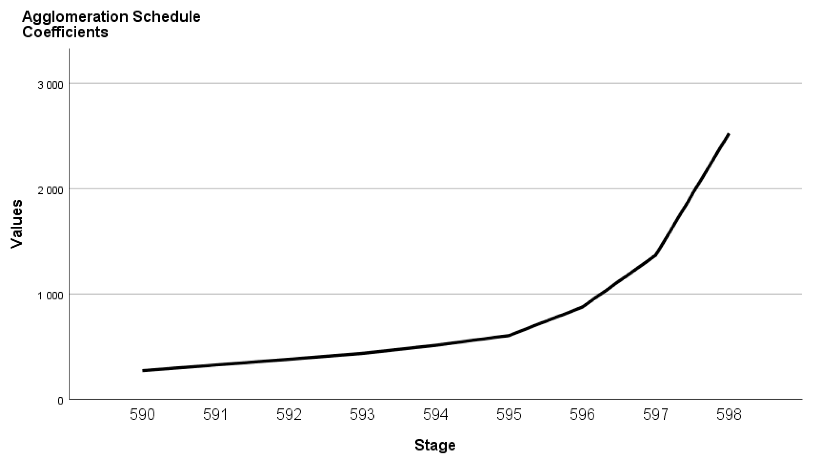
During conducting the Ward method, the groups that increase the standard deviation within the cluster the least are aggregated (
Table 5). There is a big jump when merging the last two clusters (the coefficient increasing from 1368.282 to 2527.559). The increase in coefficients during the previous merger can also be considered significant (coefficients: stage 596: 875,907 and stage 597.: 1,368,559). Based on the calculation, two or three clusters can be formed.
The increase in coefficients is also represented in
Figure 4. The horizontal axis shows the number of merging steps (Stage), while the vertical axis shows the Values (coefficients). Larger fractures can be observed on the graph, which can be considered as an elbow criterion. Based on the elbow criterion, we examined the two- and three-cluster solutions. The characterization of the clusters should first be done based on the variables applied for cluster analysis. Clusters can be interpreted based on cluster centroids (Means). Means were compared using analysis of variance, because the dependent variables are metric. Standard deviation values provide information on the extent to which homogeneous groups have been created.
Based on the two-cluster solution, the Std. deviation of AS_1 is quite large (1.90597), suggesting the weakness of group homogeneity (
Table A2—in the
Appendix A). In the case of the three-cluster solution, we can see homogeneous groups (
Table 6), since the Std. deviations have decreased compared to the two-cluster solution. Based on this, we chose a three-cluster solution.
Starting from the three-cluster solution, socio-demographic variables (gender, generation) and a variable showing the evaluation of sustainability attitudes were included in the typology, which was not used in the cluster analysis but may specify the characteristics of each cluster.
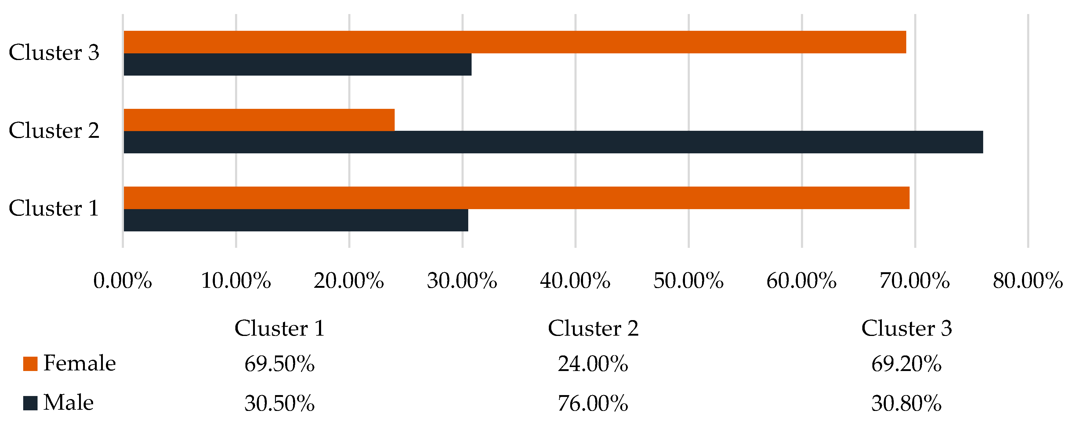
According to genders, the first and the third clusters are dominated by female respondents (
Figure 5). The second cluster has the highest proportion of male respondents (76.0%). To determine the correlation between variables, the χ2 test was performed.
Pearson’s Chi-Square Test (
Table A3—in the
Appendix A) shows that the observed value of the indicator is 2.909, which, even when examined at the bilateral significance level of 0.573 (ASYMP. SIG. (2-sided)), exceeds the theoretical threshold, i.e., the significance level is lower than the selected significance level of 0.05. Consequently, we reject that there is no correlation between the two variables. Based on the Likelihood Ratio, the relationship is significant (0.460 > 0.005), so the gender distribution correlates with the clusters formed.
According to generation variable, the dominance of the Z and Y generation respondents can be observed in all clusters. Therefore, we examined how the distribution of these two age groups changes within the clusters (
Figure 6). We can see that in the first cluster the ratio of the two age groups is quite balanced, and the role of the Z generation is slightly larger. The second cluster shows the dominance of the Y generation age group, while the third cluster shows a large potency of the Z generation.
By analysing the correlation between the variables, the observed value of the Pearson Chi-Square (
Table A4—in the
Appendix A) index is 4.456, which, even when tested at the bilateral significance level of 0.924 (ASYMP. SIG. (2-sided)), exceeds the theoretical threshold, i.e., the significance level is lower than the selected significance level of 0.05. In this case we also reject the null hypothesis that there is no correlation between the two variables. Based on the Likelihood Ratio, the relationship is significant (0.939 > 0.005), and so the age distribution is also correlated with the clusters formed.
In the first and third clusters, the importance of sustainability is below the mean value (
Table 7), but in the second cluster, we can see a much higher value (Mean: 6.3695) compared with TOTAL values (Mean: 5.0101). Based on Std. Deviation, groups can be considered relatively homogeneous (values below 2.).


