Abstract
Photovoltaic (PV) cell (PVC) modeling predicts the behavior of PVCs in various real-world environmental settings and their resultant current–voltage and power–voltage characteristics. Focusing on PVC parameter identification, this study presents an enhanced particle swarm optimization (EPSO) algorithmto accurately and efficiently extract optimal PVC parameters. Specifically, the EPSO algorithm optimizes the minimum mean squared error between measured and estimated data and, on this basis, extractsthe parameters of the single-, double-, and triple-diode models and the PV module. To examine its effectiveness, the proposed EPSO algorithm is compared with other swarm optimization algorithms. The effectiveness of the proposed EPSO algorithm is validated through simulation. In addition, the proposed EPSO algorithm also exhibits advantages such as an excellent optimization performance, a high parameter estimation accuracy, and a low computational complexity.
1. Introduction
Fossil fuels are one of the energy sources that can best accommodate human needs. Due to their low cost, high efficiency, and ease of transportation, fossil fuels have gained tremendous popularity around the globe, which has resulted in an increase in their use [1]. Despite their advantages, fossil fuels also inevitably have shortcomings [2,3]. A myriad of factors, such as excess air pollution, global warming, and the depletion of energy sources, have precipitated a global effort to develop various renewable energy sources [4], including solar energy, wind energy, hydropower, biomass energy, hydrogen and fuel cells, and geothermal energy [5,6].Of renewable energy sources, solar energy is most suitable for pure power generation on a global scale thanks to the ease of installation of its required devices and itshigh power-generation output and efficiency. Photovoltaic (PV) technology has also been designated as a focus of research by researchers and enterprises. A satisfactory PV cell (PVC) and component model is indispensable for enhancing PV system performance. There are two steps involved in PV modeling based on measured current I and voltage V data, namely, (1) mathematical modeling and (2) model parameter identification [7]. A number of models have been proposed to show the behavior of PVCs. The single-diode (SD), double-diode (DD), and triple-diode (TD) models are most frequently used [8,9,10,11]. It is necessary to accurately estimate five, seven, and ten parameters for the SD, DD, and TD models, respectively. Accurate parameter estimation can improve not only the performance of a PVC but also its control quality. To estimate PVC model parameters, equation-based analytical methods have been proposed [12,13]. These methods determine the parameters of a PVC model by solving a system of transcendental equations. Due to the nonlinear problem associated with PVC models, these methods need to simplify the unknown parameters or assume that some parameters are constants. While analytical methods only involve simple and fast calculations, their estimation accuracy is low due to assumption errors and parameter elimination. Numerical methods are used to estimate PVC model parameters by fitting the points on PV characteristic curves [14,15,16]. Compared to analytical methods, numerical methods are able to produce relatively accurate estimates. However, numerical methods involve complex calculations, and their estimation accuracy and convergence are overly reliant upon the initial value, whereasthe selection of a suitable initial value remains a difficulty. As a result, convergence of numerical methods cannot be guaranteed. PV parameter identification is a dimensionless multimodal problem. Swarm intelligence (SI) algorithms have demonstrated an exceeding performance for similar problems. Based on an overview of the available literature, the particle swarm optimization (PSO), differential evolution (DE), and artificial bee colony (ABC) algorithms are currently the most popular SI optimization algorithms [10,17,18,19,20]. Inspired by natural phenomena, these algorithms first randomly generate an initial value and subsequently use a repeated process to describe the variation in the fitness function of the problem with parameters. This process is repeated continuously until the fitness function meets the preset termination conditions, at which point satisfactory optimization results are obtained. However, these algorithms are not perfect and have their respective shortcomings. To prevent “precocity”, the DE algorithm requires a large swarm size, which results in a long computational time and affects the optimization results. The ABC algorithm is slow in convergence and imbalanced between exploration and development. The PSO algorithm is prone to falling into local optima and has a poor global optimization performance. This is because the PSO algorithm depends upon artificially preset control parameters and a single iterative updating equation. Nevertheless, compared to many other SI algorithms, the PSO algorithm is the least complex computationally and is highly capable of searching for local optimal solutions.In view of this, in this study, an adaptive adjustment strategy for control parameters is adopted to alter the motion of particles and allow them to move toward the optimal solutionsto improve the optimization ability of the PSO algorithm. Finally, the enhanced PSO (EPSO) algorithm is employed to optimize the PVC model parameters.
The remainder of this article is organized as follows. Section 2describes the problem from an optimization perspective. Section 3presentsthe EPSO algorithm (Section 3.1) andproposes an objective function for addressing PVC model parameter identification and an implementation process based on the EPSO algorithm (Section 3.2). In Section 4, the effectiveness of the proposed algorithm is demonstrated using numerical simulation. Finally, this study is summarized in Section 5.
2. Description of the Problem
2.1. SD Model
Figure 1 shows the SD PVC model (Rsh is the parallel shunt resistance of the diode, and Rs is the divider resistance of the PVC). The output I of the PVC is calculated using Equation (1).
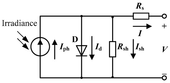
Figure 1.
Equivalent circuit for the single-diode model.
In Equation (1), is the current generated by solar illumination, is the current that passes through the diode, and is the current that passes through Rsh that reflects the cut-off of the p–n junction of the PVC. and are calculated using Equations (2) and (3), respectively.
In Equations (2) and (3), kB is the Boltzmann constant, T is the temperature of the PVC, q is the absolute value electric charge of electrons, a is the nonideal coefficient of the backward compound diode, V is the output voltage of the PVC, and Isd is the backward saturation current of the diode.
Let be the PVC model parameters to be optimized.
2.2. DD Model
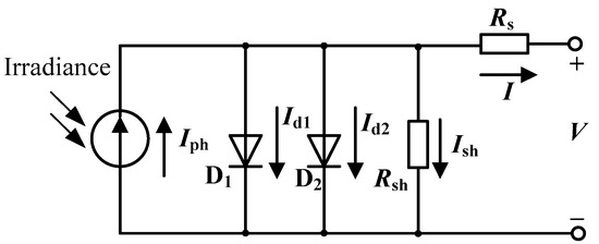
Figure 2.
Equivalentcircuit for the double-diode model.
According to the Shockley equation, and in the above equation are calculated using Equations (5) and (6), respectively.
In Equations (5) and (6), and are the diffusion and saturation currents, respectively, and and are the ideal coefficients of the diffusion and compound diodes, respectively.
Let be the DD model parameters to be optimized.
2.3. TD Model
Figure 3 shows the TD PVC model. The output I of the PVC is calculated using Equation (7).
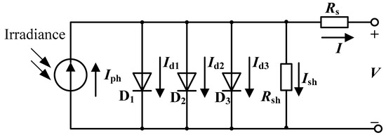
Figure 3.
Equivalentcircuit for the three-diode model.
According to Khanna et al. [10], , , and in the above equation are calculated using Equations (8)–(10), respectively.
Based on Equations (8)–(10), Rs is no longer considered to remain unchanged as the load I changes; instead, it is considered to be a variable parameter, the value of which depends upon the changes in I. To determine Rs, it is necessary to determine its relationship with I, i.e., to calculate Rso and K.
Let be the TD model parameters to be optimized.
2.4. PV Module Model
A PV module is composed of PVCs connected in parallel or in series. Figure 4 shows an equivalent SD circuit of a PV module. The output I of the PV module is calculated using Equation (11).

Figure 4.
Equivalent circuit for the PV module.
In Equation (11), and are the numbers of PVCs connected in parallel and series, respectively. Let be the model parameters to be optimized.
3. Materials and Methods
3.1. EPSO Algorithm
PSO is a swarm-based optimization technique proposed by Kennedy and Eberhart, who were inspired by social behaviors related to swarms (e.g., bird swarms). A particle swarm is composed of a large number of particles. Each particle represents a possible solution to the optimization task and attempts to search for an optimal location by flying in a multidimensional space. In the optimization process, each candidate solution is determined by two vectors, namely, a location vector and a speed vector, in the multidimensional search space. Each particle in the swarm is updated based on the abovementioned attributes. The speed and location of each particle are updated using Equations (12)–(14), respectively. Figure 5 shows the PSO process (the arrowed solid and dotted lines represent one iteration and multiple iterations, respectively).
where l = 1, 2, …, Np (Np is the particle swarm size), d = 1, 2, …, D (D is the dimension of the optimal solution), k = 1, 2, …, kmax (kmax is the maximum number of iterations), denotes the optimal solution for the lth particle up to the present, denotes the overall optimal solution for the particles up to the present, r1 and r2 are random numbers between −1 and 1, and c1 and c2 are cognitive and social parameters, respectively. The following values are required: c1 + c2= 0.4, , and .
Figure 5.
Particle’smovement of original PSO algorithm.
It is well known that the PSO algorithm is prone to falling into local optima. To overcome this disadvantage, the mechanism in Figure 6 is adopted in this study to improve the convergence speed and global optimization performance of the PSO algorithm. The improved PSO algorithm is referred to as the EPSO algorithm. The following section describes the EPSO algorithm.
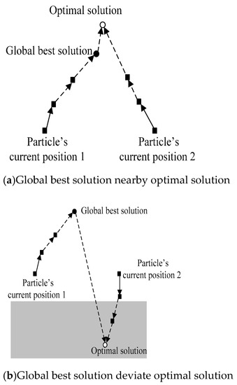
Figure 6.
Particle’smovement of enhanced PSO algorithm.
Initialization. As with all the swarm-based optimization algorithms, swarm initialization is a vital task for the EPSO algorithm because it affects the convergence speed and the quality of the ultimate solution. In the absence of prior knowledge, random number generation is a method commonly used to create an initial swarm. Thus, as discussed by Wang [17], an opposition-based learning method can be employed to obtain a more suitable initial candidate solution, even if no prior knowledge of the solution is available. Equation (15) shows the swarm initialization used in this study.
where rand is a random number between −1 and 1, and are the maximum and minimum values of the candidate solution in the dth dimension, respectively, and is the initial value.
Particle motion update. In this study, Equations (16) and (17) are used to describe the updating of particle motions.
In Equations (16) and (17), k is the number of iterations, ls is a number randomly selected from the range of [1 Np], which must differ from l (i.e., ls≠l), , , and are the increments in each iteration, and , , and are the iteration step sizes corresponding to , , and , respectively. The adaptive update strategy described in Equations (18)–(20) is adopted in this study.
where is generated within the range of [μF, 0.1] based on the Cauchy distribution function, and μF is updated using Equation (19) (the initial value of μF is set to 0.5).
where c is a constant factor (), and is the Lehmer mean that has successfully allowed the objective function to obtain a further optimized set, which is calculated using Equation (20).
where is the further optimized set that is successfully obtained by the objective function, and is the ith element in .
After a new candidate solution is generated, it is evaluated by the particle. The performance of the new candidate solution is compared with that of the old candidate solution. If the quality of the new optimal solution is the same as or better than that of the old optimal solution, the individual optimum is replaced by the new optimal solution; otherwise, the old optimal solution is preserved. If the number of times when the candidate solution cannot be further improved reaches the preset value, the particle location is discarded and Equation (21) is used to generate a new location for the discarded particle.
where is the upper limit number of cycles when the candidate solution cannot be further improved, and is the counter for the number of times when the location of the lth particle is not improved.
The adaptive update strategy described in Equations (18)–(20) is based on an optimized objective function and offers notable guidance. It is hoped that this adaptive update strategy, combined with Equations (16), (17), and (21), can prevent the PSO algorithm from falling into “precocity,” allow it to obtain a global optimal solution, and improve its convergence speed.
3.2. PVC Model Parameter Identification Based on The EPSO Algorithm
The main objective of PVC model parameter identification is to search for optimal values for the unknown parameters to minimize the difference between measured and calculated I data. Forthe SD, DD, and TD models and a PV module, the difference between the measured and estimated I data of each pair is defined by Equations (22)–(25), respectively. The overall difference is quantified using the mean squared error (MSE) in Equation (26).
where t = 1, 2, …, tmax (tmax is the time-domain sampling point).
Parameter identification is a process that minimizes the MSE between measured and calculated data by adjusting the model parameters. Manifestly, the smaller is, the more accurate the model is. In this study, the code of the PVC parameters is treated as a candidate solution θ, and the EPSO algorithm is employed to calculate the minimum value of each of Equations (22)–(26). Algorithm 1 summarizes the pseudocode of the implementation of the EPSO algorithm for PVC parameter identification. Figure 7 shows the flowchart of PVC parameter identification using the EPSO algorithm.
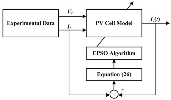
Figure 7.
Overview for parameters estimation of PV Cell models using EPSO algorithm.
| Algorithm 1. Pseudocodeof parameter identification for a solar cell using EPSO. |
 |
4. Simulation Experiments
This section presents a series of simulation experiments conducted to evaluate the performance of the algorithm proposed in this study. The data used in Experiments 1, 2, and 3 were obtained by testing commercially available RTC France silicon PVCs under standard conditions(irradiance: 1000 W/m2; temperature: 33 °C) by T.Easwarakhanthan [21,22,23]. A DPL Photowatt-PWP201 PV module composed of 36 polycrystalline silicon cells connected in series [24] was used in Experiment 4. The data used in Experiment 4 were obtained at an irradiance of 1000 W/m2 and a temperature of 45°C.To better examine the effectiveness of the parameter identification algorithm proposed in this study, the experimental results were compared with those obtained using the PSO algorithm [10], an improved PSO (IPSO) algorithm [20], the DE algorithm [19], and the ABC algorithm [18]. Equations (27)–(31) show the control parameter settings for the EPSO, PSO, IPSO, DE, and ABC algorithms, respectively. Table 1 summarizes the computational load of each algorithm. Table 2 summarizes the value ranges of the PVC parameters to be identified. All the experiments were conducted on the same hardware (dual Intel Core i-9700 3.0 GHz central processing unit; 16 GB of memory). Please note that the simulation results are the average values obtained from 20 independent operations [25].

Table 1.
Operation requirements of different swarm optimization algorithms.
Table 2.
Upper and lower range of the solar cell parameters.
4.1. Experiment 1 SD Model
The five SI algorithms were used to identify the parameters of the SD model. Figure 8 shows the convergence curve of each algorithm. Table 3 summarizes the convergence value and running time of each algorithm. To quantitatively evaluate the estimation performance of each algorithm, Equations (32) and (33) were used to evaluate the estimation results. Figure 9 and Table 4 show the comparison of the current estimates given by the algorithms. Figure 10 shows the powerP–V characteristic curves of the SD model calculated using the various algorithms.
where t = 1, 2, …, tmax, is the relative error of the estimated current, and is the operator for calculating the absolute value.
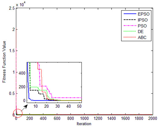
Figure 8.
J(α) evolution of different algorithm for the single-diode model.
Table 3.
J(α)and cost time of different swarm optimization algorithms for the single-diode model.
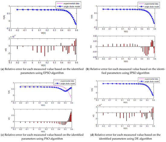
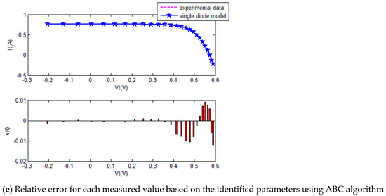
Figure 9.
The comparison of the results of five methods for the single-diode model.
Table 4.
Curve fitting results of different method for the single-diode model.
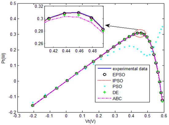
Figure 10.
Measured voltage vs. power of five algorithm for the single-diode model.
The convergence curves of the various algorithms in Figure 8 were plotted based on the average values of obtained from 20 independent operations. Evidently, the EPSO algorithm converged faster than the other algorithms. A comparison of the algorithms in terms of the convergence values and computational times is presented in Table 3. The PSO algorithm had the shortest computational times but the worst convergence values. The EPSO and DE algorithms exhibited the same convergence values for the SD model, whereas the computational times of the DE algorithm were nearly five times those of the EPSO algorithm. In addition, it is worth noting that the convergence values of the EPSO algorithm were the lowest of all the algorithms used to identify the parameters of the single-diode model. This finding further demonstrates that the EPSO algorithm outperformed the other algorithms in terms of convergence. A comparison of the I–V characteristic curves in Figure 9, the P–V characteristic curves in Figure 10, and the output I (Ier) values in Table 4 show that the I–V and P–V characteristic curves and the Ier values of the PVCs estimated by the proposed algorithm were closer to the measured data. This finding suggests that the EPSO-based PVC parameter identification algorithm has a higher identification accuracy.
4.2. Experiment 2 DD Model
The five SI algorithms were used to identify the parameters of the DD model. Figure 11 shows the convergence curve of each algorithm. Table 5 summarizes the convergence value and running time of each algorithm. Equations (32) and (33) were used to quantitatively evaluate the current estimates. Figure 12 and Table 6 show the current estimates. Figure 13 shows the P–V characteristic curves of the DD model calculated using the various algorithms.
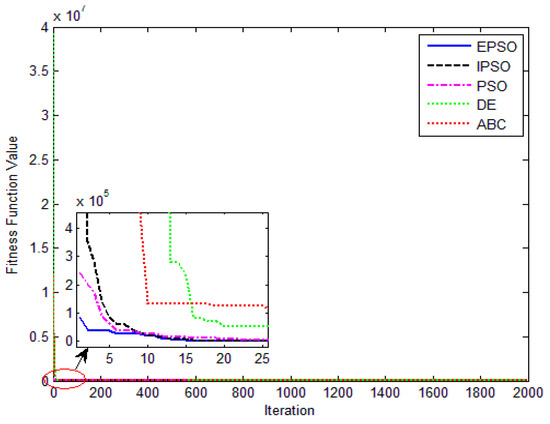
Figure 11.
J(α) evolution of different algorithm for the double-diode model.
Table 5.
J(α) and cost time of different swarm optimization algorithms for the double-diode model.
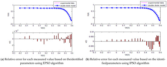
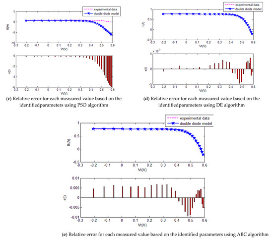
Figure 12.
The comparison of the results of five methods for the double-diode model.
Table 6.
Curve fitting results of different method for the double-diode model.
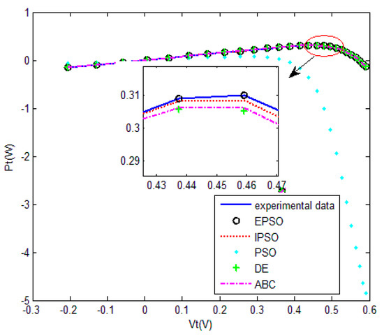
Figure 13.
Measured voltage vs. power of five algorithm for the double-diode model.
The convergence curves of the various algorithms in Figure 11 were plotted based on the average values of obtained from 20 independent operations. Evidently, the EPSO algorithm converged fastest. A comparison of the algorithms in terms of the convergence values and computational times is shown in Table 5,where the PSO algorithm had the shortest computational times but the worst convergence values. The computational times of the PSO algorithm were nearly three times those of the EPSO algorithm. In addition, it is worth noting that the convergence values of the EPSO algorithm were the lowest of all the algorithms used to identify the parameters of the double-diode model. This finding further demonstrates that the EPSO algorithm outperformed the other algorithms in terms of convergence. A comparison of the I–V characteristic curves in Figure 12, the P–V characteristic curves in Figure 13, and the output I (Ier) values in Table 6 show that the I–V and P–V characteristic curves and the Ier values of the PVCs estimated by the proposed algorithm were closer to the measured data.
4.3. Experiment 3 TD Model
The five SI algorithms were used to identify the parameters of the TD model. Figure 14 shows the convergence curves. Table 7 summarizes the convergence value and running time of each algorithm. Figure 15 and Table 8 show the current estimates. Figure 16 shows the P–V characteristic curves of the TD model calculated using the various algorithms.
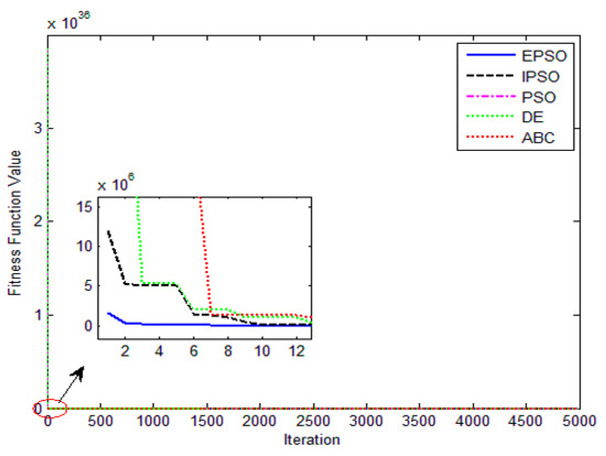
Figure 14.
J(α)evolution of different algorithm for the triple-diode model.
Table 7.
J(α) and cost time of different swarm optimization algorithms for the triple-diode model.
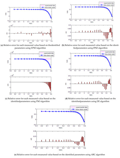
Figure 15.
The comparison of the results of five methods for the triple-diode model.
Table 8.
Curve fitting results of different method for the triple-diode model
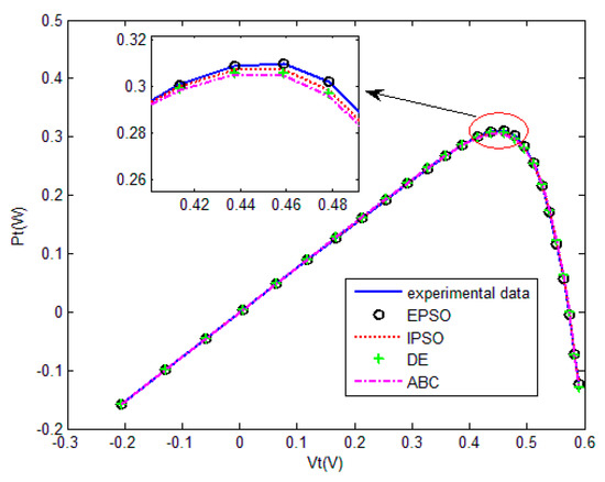
Figure 16.
Measured voltage vs. power of five algorithm for the triple-diode model.
The convergence curves of the various algorithms in Figure 14 were plotted based on the average values of obtained from 20 independent operations. Obviously, the EPSO algorithm converged faster than the other algorithms. A comparison of the algorithms in terms of the convergence values and computational times are presented in Table 7. The PSO algorithm had the shortest computational times but the worst convergence values, whereas the computational times of the ABC algorithm were nearly six times those of the EPSO algorithm. In addition, it is worth noting that the convergence values of the EPSO algorithm were the lowest of all the algorithms used to identify the parameters of the single-diode model. This finding further demonstrates that the EPSO algorithm outperformed the other algorithms in terms of convergence. A comparison of the I–V characteristic curves in Figure 15, the P–V characteristic curves in Figure 16, and the output I (Ier) values in Table 8 show that the I–V and P–V characteristic curves and the Ier values of the PVCs estimated by the proposed algorithm were closer to the measured data.
4.4. Experiment 4PV Module Model
The five SI algorithms were used to identify the parameters of the Photowatt-PWP201 PV module model. Figure 17 shows the convergence curves. Table 9 summarizes the convergence value and running time of each algorithm. Figure 18 and Table 10 show the current estimates. Figure 19 shows the P–V characteristic curves of the PV module calculated using the various algorithms.
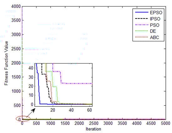
Figure 17.
J(α) evolution of different algorithm for the PV module.
Table 9.
J(α) and cost time of different swarm optimization algorithms for the PV module.
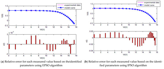
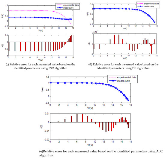
Figure 18.
The comparison of the results of five methods for the PV module.
Table 10.
Curve fitting results of different method for the PV module.
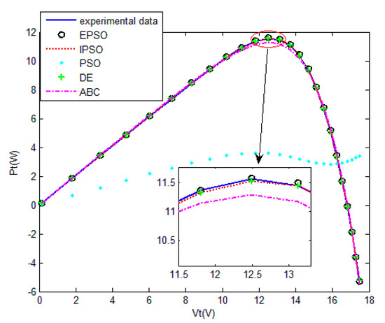
Figure 19.
Measured voltage vs. power of five algorithm for the PV module.
The convergence curves of the various algorithms in Figure 17 were plotted based on the average values of obtained from 20 independent operations. Evidently, the EPSO algorithm converged faster than the other algorithms. A comparison of the algorithms in terms of the convergence values and computational times in Table 9 shows the following. The PSO algorithm had the shortest computational times but the worst convergence values. The EPSO and DE algorithms exhibited the same convergence values for the the PV module, whereas the computational times of the DE algorithm were over five times those of the EPSO algorithm. In addition, it is worth noting that the convergence values of the EPSO algorithm were the lowest of all the algorithms used to identify the parameters of each model. This finding further demonstrates that the EPSO algorithm outperformed the other algorithms in terms of convergence. A comparison of the I–V characteristic curves in Figure 18, the P–V characteristic curves in Figure 19, and the output I (Ier) values in Table 10, show that the I–V and P–V characteristic curves and the Ier values of the PVCs estimated by the proposed algorithm were closer to the measured data. This finding suggests that the EPSO-based PVC parameter identification algorithm has a higher identification accuracy and the other algorithms.
5. Conclusions
The maindifficultyin accurately modeling a PVC is the lack of accurate parameter information that describes the characteristics of the PVC. This study presents an EPSO algorithm equipped with an effective update mechanism to accurately and efficiently extract PVC model parameters. To better examine its effectiveness, the EPSO algorithm was compared with other SI optimization algorithms. In addition, the quality of the identified parameters was also evaluated. The results show that the I–V and P–V characteristics calculated using the EPSO algorithm agreed satisfactorily with the test data. Moreover, the EPSO algorithm was also found to outperform the other swarm optimization algorithms.
Funding
This research was funded by National Natural Science Foundation of China under Grant No.51879118, High-Level Talent Training Project in The Transportation Industry under Grant No.2019-014, Natural Science Foundation of Fujian Province under Grant No.2020J01688, Foundation of Fujian Education Committeeof China for New Century Distinguished Scholars under Grant No. B17159, Scientific Research Foundation of Key Laboratory of Fishery Equipment and Engineering, Ministry of Agriculture of the People’s Republic of China under Grant No.2016002 and 2018001, Scientific Research Foundation of Artificial Intelligence Key Laboratory of Sichuan Province under Grant No.2017RYJ02, and Scientific Research Foundation of Jiangsu Key Laboratory of Power Transmission & Distribution Equipment Technology under Grant No. 2017JSSPD01.
Institutional Review Board Statement
The study was not involve humans or animals.
Informed Consent Statement
The study was not involve humans or animals.
Data Availability Statement
The data used to support the findings of this study are available from the corresponding author upon request.
Conflicts of Interest
The authors declare no conflict of interest.
References
- Femia, N.; Petrone, G.; Spagnuolo, G.; Vitelli, M. Power Electronics and Control Techniques for Maximum Energy Harvesting in Photovoltaic Systems; CRC Press: Boca Raton, FL, USA, 2012. [Google Scholar]
- Batzelis, E.I.; Kampitsis, G.E.; Papathanassiou, S.A.; Manias, S.N. Direct MPP Calculation in Terms of the Single-Diode PV Model Parameters. IEEE Trans. Energy Convers. 2015, 30, 226–236. [Google Scholar] [CrossRef]
- Chin, V.J.; Salam, Z.; Ishaque, K. Cell modelling and model parameters estimation techniques for photovoltaic simulator application: A review. Appl. Energy 2015, 154, 500–519. [Google Scholar] [CrossRef]
- Jin, T.; Kim, J. A comparative study of energy and carbon efficiency for emerging countries using panel stochastic frontier analysis. Sci. Rep. 2019, 9, 6647. [Google Scholar] [CrossRef]
- Ridha, H.M.; Gomes, C.; Hazim, H.; Ahmadipour, M. Optimal Design of Standalone Photovoltaic System Based on Multi-Objective Particle Swarm Optimization: A Case Study of Malaysia. Processes 2020, 8, 41. [Google Scholar] [CrossRef]
- Mohammed, R.H.; Gomes, C.; Hizam, H. Multiple scenarios multi-objective salp swarm optimization for sizing of standalone photovoltaic system. Renew. Energy 2020, 153, 1330–1345. [Google Scholar]
- Ram, J.P.; Babu, T.S.; Dragicevic, T.; Rajasekar, N. A new hybrid bee pollinator flower pollination algorithm for solar PV parameter estimation. Energy Convers. Manag. 2017, 135, 463–476. [Google Scholar] [CrossRef]
- Tsai, H.-L. Insolation-oriented model of photovoltaic module using Matlab/Simulink. Sol. Energy 2010, 84, 1318–1326. [Google Scholar] [CrossRef]
- Saloux, E.; Teyssedou, A.; Sorin, M. Explicit model of photovoltaic panels to determine voltages and currents at the maximum power point. Sol. Energy 2011, 85, 713–722. [Google Scholar] [CrossRef]
- Khanna, V.; Das, B.K.; Bisht, D.; Vandana; Singh, P. A three diode model for industrial solar cells and estimation of solar cell parameters using PSO algorithm. Renew. Energy 2015, 78, 105–113. [Google Scholar] [CrossRef]
- Montano, J.; Tobón, A.; Villegas, J.P.; Florez, M.D. Grasshopper optimization algorithm for parameter estimation of photovoltaic modules based on the single diode model. Int. J. Energy Environ. Eng. 2020, 11, 367–375. [Google Scholar] [CrossRef]
- Lun, S.-X.; Du, C.-J.; Yang, G.-H.; Wang, S.; Guo, T.-T.; Sang, J.-S.; Li, J.-P. An explicit approximate I–V characteristic model of a solar cell based on padé approximants. Sol. Energy 2013, 92, 147–159. [Google Scholar] [CrossRef]
- Liu, S.; Shu, S.X.; Chao, C.J. A new explicit I-V model of a solar cell based on Taylor’s series expansion. Sol. Energy 2013, 94, 221–232. [Google Scholar]
- Yetayew, T.T.; Jyothsna, T.R. Parameter extraction of photovoltaic modules using Newton Raphson and simulated annealing techniques. In Proceedings of the 2015 IEEE Power, Communication and Information Technology Conference (PCITC), Bhubaneswar, India, 15–17 October 2015; pp. 229–234. [Google Scholar]
- Ghani, F.; Fernandez, E.F.; Almonacid, F. The numerical computation of lumped parameter values using the multi-dimensional Newton-Rapson method for the characterization of a multi-junction CPV module using the five-parameter approach. Sol. Energy 2017, 149, 302–313. [Google Scholar] [CrossRef]
- Tossa, A.K.; Soro, Y.; Azoumah, Y.; Yamegueu, D. A new approach to estimate the performance and energy productivity of photovoltaic modules in real operating conditions. Sol. Energy 2014, 110, 543–560. [Google Scholar] [CrossRef]
- Wang, R.J. Application of Artificial Bee Colony; Publishing House of Electronics Industry: Beijing, China, 2016. [Google Scholar]
- Oliva, D.; Cuevas, E.; Pajares, G. Parameter identification of solar cells using artificial bee colony optimization. Energy 2014, 72, 93–102. [Google Scholar] [CrossRef]
- Chellaswamy, C.; Ramesh, R. Parameter extraction of solar cell models based on adaptive differential evolution algorithm. Renew. Energy 2016, 97, 823–837. [Google Scholar] [CrossRef]
- Nunes, H.G.G.; Pombo, J.A.N.; Mariano, S.J.P.S. A new high performance method for determining the parameters of PV cells and modules based on guaranteed covergence particle swarm optimization. Appl. Energy 2018, 211, 774–791. [Google Scholar] [CrossRef]
- Kenndy, J.; Eberhart, R. Particle swarm optimization. In Proceedings of the IEEE International Conference on Neural Networks, Perth, Australia, 27 November–1 December 1995; pp. 1942–1948. [Google Scholar]
- Wang, R.; Zhan, Y.; Haifeng, Z. A Class of Sequential Blind Source Separation Method in Order Using Swarm Optimization Algorithm. Circuits Syst. Signal Process. 2015, 35, 3220–3243. [Google Scholar] [CrossRef]
- Easwarakhanthan, T.; Bottin, J.; Bouhouch, I.; Boutrit, C. Nonlinear Minimization Algorithm for Determining the Solar Cell Parameters with Microcomputers. Int. J. Sol. Energy 1986, 4, 1–12. [Google Scholar] [CrossRef]
- Luque, A.; Hegedus, S. Handbook of Photovoltaic Science and Engineering; John Wiley & Sons: New York, NY, USA, 2010. [Google Scholar]
- DPL Energy Tech. Co., Ltd. The Data of Solar Cells. Available online: http://www.dpl-energy.com (accessed on 27 August 2020).


Publisher’s Note: MDPI stays neutral with regard to jurisdictional claims in published maps and institutional affiliations. |
© 2021 by the author. Licensee MDPI, Basel, Switzerland. This article is an open access article distributed under the terms and conditions of the Creative Commons Attribution (CC BY) license (http://creativecommons.org/licenses/by/4.0/).