
Whose Happiness in Which Cities? A Quantile Approach


School of Geography, Environment and Earth Sciences, Victoria University of Wellington, Wellington 6140, New Zealand
Sustainability 2021, 13(20), 11290; https://doi.org/10.3390/su132011290
Submission received: 6 May 2021
/
Revised: 9 September 2021
/
Accepted: 22 September 2021
/
Published: 13 October 2021
(This article belongs to the Special Issue Happy and Healthy Cities)
Abstract
:The proposition that living in the largest urban agglomerations of an advanced economy reduces the average wellbeing of residents is known as the urban wellbeing paradox. Empirical tests using subjective wellbeing have produced mixed results and there are two reasons for being cautious. Firstly, the default reliance on the conditional mean can disguise uneven effects across the wellbeing distribution. Secondly, relying on respondents to define their settlement size does not ensure a consistent measure of the agglomeration. I therefore apply quantile regression to the life satisfaction and happiness measures of wellbeing as collected by the 2018 European Social Survey (ESS9) and employ a consistent local labour market-based definition of agglomeration—The Functional Urban Area (FUA). I compare three countries as proof of concept: one with a known strong negative (respondent defined) agglomeration effect (Austria), one with a slight negative effect (Czech Republic), and one where living in the main agglomeration is positively associated with average wellbeing (Slovenia). The uneven wellbeing effect of living in the largest agglomeration in each country raises questions about who benefits in which cities.
1. Introduction
Of particular interest in wellbeing studies is the way in which people’s attributes interact with their place of residence to affect their subjective wellbeing [1,2,3,4,5]. One such thesis is that average wellbeing rises with urban residence in developing countries but falls with residence in the largest urban agglomerations of developed economies, a phenomenon known as the urban wellbeing paradox. In addition to its distributional implications this spatial patterning is of interest because, if sustained, continued growth of the agglomeration would further reduce the likelihood of wellbeing rising-independent of the failure of growth to alter people’s social rank [6,7].
The following paper is guided by two questions. The first asks whether those living within the largest urban centres of developed countries in Europe do in fact return lower average levels of wellbeing—hypothesis 1 (H1). The second asks whether the influence of residence within the agglomeration is evenly felt across the wellbeing distribution (H2).
The study makes two contributions. The first is to offer partial support for H1 by showing that the majority of the nearly thirty countries covered by the European Social Survey 2018 do still report lower levels of wellbeing in their so called ‘Big Cities’ compared to the rest of the country. The second is to reject H2 by showing that the effect of agglomeration on the mean of wellbeing masks considerable heterogeneity across the wellbeing distribution of each of the three main cities.
2. Materials and Methods
Urbanisation remains a primary instrument in the quest for economic growth and on those grounds alone one would expect residence in successively larger and richer urban clusters to be associated with higher levels of subjective wellbeing. While higher wellbeing is typical of cities in developing countries [8], it is not necessarily the case in developed economies where, “the urban happiness advantage is less and sometimes negative in countries at the top of the happiness distribution” [9] (Figure 1.2). Instead of average wellbeing rising with the increased specialisation that urban size allows, average wellbeing is actually lower in many if not all of these largest urban centres [2] (pp. 790–791). As others have reflected, such “cities provide sought-after resources, but we pay a price: the relative unhappiness of city life” [10] (p. 11).
The term ‘urban paradox’ has been used in the above context to refer to the fact that urban wealth is not adequately translated into job creation [11] (p. 191). In this paper I focus on the related urban wellbeing paradox, which refers to the lower average subjective wellbeing inside the major urban agglomeration of the country.
The statistical association between subjective wellbeing and urban settlement has now received attention worldwide [8,9] particularly in Europe: Norway [12,13], Sweden [14], Finland [5,15], the United Kingdom [16,17,18,19,20], Ireland [21], Germany [22,23], Switzerland [24], Italy [25,26], Spain [27], Romania [28,29] and, most recently, Slovakia [30]. While many European studies offer empirical support for the paradox others draw attention to the highly conditional nature of the proposition. Notable by its absence in this line up is France (although see [31,32,33]). At the same time, several studies have addressed variations in subjective wellbeing across Europe as a whole, by country, NUTS (Nomenclature des Unités territoriales statistiques) regions or urban area. Examples include [10,34,35,36,37,38,39,40,41,42,43,44].
Although a pan-European pattern of urbanisation has developed with a core of high population density stretching from London through the Ruhr Valley to Northern Italy, the history and the current economic and institutional structure of individual countries retains a considerable hold on the way country populations are distributed across their respective urban hierarchies. I draw on the 29 countries surveyed in the ninth 2018 wave of the European Social Survey (ESS9) as listed in Table 1. There is a marked variation in their populations ranging from Germany with close to 82.3 million (in 2018) to Iceland with less than half a percent of that number (0.32 million); in fact, 25 of the 29 countries in the ESS9 had less than half the population of Germany. There is no apparent relationship between their level of urbanisation and their population size.
The three countries used as case studies in this paper come from each third of the population size distribution. Appearing in bold in Table 1 they are Czech Republic (10.6 million), Austria (8.7 million) and Slovenia (2 million). Columns 3 and 4 carry the urban and rural populations as defined separately by each country. The urbanisation rates of the three case studies range from 54.5 percent in Slovenia to 58.3 percent in Austria and 73.8 percent in Czech Republic.
The European Social Survey is one of several publicly available surveys used to investigate subjective wellbeing within and between European countries, its primary attraction being its large sample size and 11-point scaling of the wellbeing variables as well as its rich range of explanatory variables—over 150 questions collected from almost 30 countries every second year. Of immediate relevance are the responses to two subjective wellbeing questions. The first is the life satisfaction question: “All things considered, how satisfied are you with your life as a whole nowadays? Please answer using this card, where 0 means extremely dissatisfied and 10 means extremely satisfied”. Refusal and ‘do not know’ were also options (B27, Card 11).
The second is the happiness question which asks: “Taking all things together, how happy would you say you are? Please answer using this card, where 0 means extremely unhappy and 10 means extremely happy. Refusal and ‘do not know’ were also options, (C1, Card 19).
Life satisfaction is a cognitive, reflective measure [45,46] whereas the happiness question elicits a measure of affect or mood. Both variables have been widely used and scrutinised [47,48]. Although they assume similar distributions in aggregate several studies have documented their weak correlation at the level of the individual [49,50,51]. Although the two instruments are not specifically designed to pick up eudaimonic features of wellbeing [52], the high ends of both life satisfaction and happiness have been found to be highly correlated with flourishing [53].
Proponents of the urban wellbeing paradox argue that citizens report lower average levels of subjective wellbeing in their largest most populous urban settlement. However, until recently, few surveys including the ESS have attempted to capture the actual location of the respondent beyond recording the NUTS regions in which they are resident (see Appendix A). NUTS regions carry only approximate information about their level of urbanisation and while they may correspond to particular ‘cities’ (such Wein in Austria), this correspondence is not consistent across countries. Instead, the ESS have asked respondents to classify their domicil as either a Big City, its suburbs or outskirts, a Town or a small city, a Country Village, or a Farm or Home in the countryside (ESS: question F14, Card 38).
Given my focus on urban agglomeration I have grouped the first two and last two domicil categories to create a three-category profile. Table 2 shows how the proportions living in the Big Cities and Suburbs range from 40.1 in Czechia, 31.5 in Austria and 24.8 percent in Slovenia.
As subjective judgements, there is plenty of room for the ESS9 respondent’s choice of domicil to pass through personal, cultural and historical filters before being expressed. However any comparison of domicils across countries requires we make the grand assumption that respondents interpret each category consistently from one country to another (so that a Big City means the same thing in the UK as it does in Iceland for example). A further problem in using these categories to define urbanisation is that they are not geographically bounded. Big Cities are identified by respondents at a variety of locations in most European countries. Despite this lack of precision, respondent defined settlement categories have been employed by several students of the urban wellbeing paradox as I illustrate in Appendix A.
The above reservations notwithstanding, and in the absence of an alternative, I have undertaken an initial bivariate test of the agglomeration effects on subjective wellbeing based on the ESS domicil using Equation (1).
where is the measure of wellbeing returned by the ith respondent living in the gth country and is the binary indicator of the defined agglomeration (1 for inside and 0 for outside). The defined agglomeration in the first application of Equation (1) this case is the Big City of which there are several in most countries. The α and β are parameters to be estimated and is the standard error term.
I applied Equation (1) using designated sample survey weights for each of the 29 countries [54]. I then ranked the countries according to the size of their estimated agglomeration parameter . The result in Figure 1 shows that in more than half of the countries (17 out of 29) the residents of the Big Cities had an average life satisfaction below the rest of their country. However, as Figure 1 shows, there is a wide spread above and below the dotted line of no difference (0). The rankings when happiness is used as a measure of wellbeing are very similar.
The evidence in Figure 1 is a challenge to the proponents of the urban wellbeing paradox. However, Equation (1) is not a very rigorous test because the paradox thesis only applies to a country’s largest urban complex. In order to specify a more appropriate measure of agglomeration in the following case studies I replace respondents’ subjective identification of their domicil by the objectively defined Functional Urban Area (FUA) which consists of “a densely inhabited city and a less densely populated commuting zone whose labour market is highly integrated with the city” [55,56].
By tracing the full extent of the spatially integrated housing, labour and consumption markets the FUA recognises not only the influence market size has on specialisation and productivity but also the range of ways the urban complex can influence the life satisfaction and happiness of its residents. By bringing smaller towns and villages into its orbit the Functional Urban Area also addresses the problem of small nearby centres ‘borrowing size’ in ways which blur the behavioural consequences of agglomeration [57].
By the end of September 2021 FUAs had been constructed for 24 of the 29 countries in Figure 1 and the three case studies used in this paper are confined to that subset. I begin with Austria, which according to Figure 1, registers the most marked negative effect of Big City residence, then Czech Republic which sits midway up the ranked distribution and then Slovenia where the Big City effect on wellbeing is positive.
3. Results
There is no automatic linking of residence in the FUA with responses the ESS collects on individuals and, until such connections are set up, we have to rely on linking through their NUTS region. To illustrate, Austria is divided into the nine NUTS 2 regions shown in the lower map of Figure 2. Vienna is the only ‘large metropolitan area’ defined as such by the Austrian FUA classification (upper map showing the core plus commuting zones of each FUA). It contains 2.78 million of the country’s 8.75 million people, 63 percent of whom live in the core of the urban region. Vienna has its own NUTS2 region (AT13, Wein) but its Functional Urban Area spreads considerably wider covering most of those living in AT12 as well as AT13 two thirds of whom classify their domicil as a Big City or ‘Suburbs or outskirts of Big City’.
In order to assess how sensitive the two wellbeing measures are to alternative definitions of agglomeration I estimate Equation (1) using five separate definitions. These are constructed by interacting the ESS9 domicil classification with the FUA. In the first definition Big City = 1 if respondents say they live in a Big City and 0 otherwise. Under the second definition Big City Sub = 1 if ESS9 respondents live in either the country’s Big City or its suburbs or outskirts, and 0 otherwise. Thirdly, Vienna City = 1 if they reside within Vienna FUA and say they live in a Big City and 0 otherwise. Fourthly, Vienna Sub = 1 if respondents reside within the Big City or suburbs of the Vienna FUA. Finally, Vienna FUA = 1 if respondents are resident within AT12 or AT13 and 0 otherwise.
Table 3a shows that living in urban areas has a negative effect on life satisfaction in Austria regardless of which definition of agglomeration is used (sample sizes are in parentheses). However, the results for the Big City and Big City and Suburbs categories illustrate the way the negative effect on wellbeing diminishes as urban density falls. The lowest mean life satisfaction is recorded by those who define their domicil as the Big City (regardless of where they live within the country)—at just over one half of a unit lower than those living in the other domicils, column 1 ( = −0.520). The reduction is only slightly lower if the definition is extended to include the suburbs as shown in column 2 (−0.449). The negative effect of residing in Austria’s FUA therefore supports my first hypothesis, H1, as it relates to both life satisfaction and happiness.
The association between agglomeration and happiness is not a simple replication of the life satisfaction experience. When it comes to living in Vienna City, the negative association with the short term measure of affect or happiness is considerably more marked (−0.538 **). Compared to the set of all Big Cities in Austria the difference is sustained as Vienna City is expanded to include its suburbs and further to the full FUA. This stronger negative effect of agglomeration on happiness is reflected in the larger share of the variation accounted for by the FUA in the happiness case; R2 = 0.026 > 0.016.
Despite decades of research, the reasons for the lower life satisfaction and happiness in the largest urban centres of many developed economies remain opaque and one possible explanation may have to do with the common reliance on the average person, on the mean of the respective wellbeing distribution. While the standard deviation and associated measures of wellbeing inequality have been addressed in other contexts (as reviewed in [58]) they have rarely featured in discussions of the urban wellbeing paradox (although see [8]).
3.1. The Wellbeing Distribution
The distribution of life satisfaction inside the Vienna FUA has a survey weighted mean life satisfaction mean of 7.65 (SE = 0.09, SD = 1.77) compared to 8.11 (SE = 0.06, SD = 1.78) in the rest of Austria. The picture is very similar in the case of happiness (7.58 < 8.12). The spread of the two distributions is similar. In both cases the smoothed (kernel) density plot inside Vienna FUA sits to the left of those living outside the FUA as shown in panel a of Figure 3. Their re-expression as quantile plots in panel b of Figure 3 highlights the relationship between life satisfaction scores on the Y axis and their corresponding quantiles on the X axis.
There are various reasons why living within a country’s major agglomeration might be associated with lower average wellbeing although there is little consensus in the literature as noted above. Some may have to do with the objective characteristics of the urban settlement itself in [59], but as Ala-Mantila et al. note, the spatial attributes are often overshadowed by the social connection variables [5]. Partly for this reason, the following regression models only control for the personal characteristics of those completing the ESS9.
3.2. A Multivariate Test
There is a broad consensus about the way personal attributes raise or lower average levels of wellbeing [60]. In order to control for the selection of people into the main FUA of a country I add four standard categories of covariates: demographics (D), main activity (V), human capital (H), and social capital (S). The variables W and A refer to wellbeing and agglomeration as defined in Equation (1) and the g country subscript is now implicit.
The parameter β retains its interpretation as the agglomeration effect, the vector λ carries the influence of age, sex and birthplace and η the impact of being engaged in paid work (or study), unemployment (or sickness), retirement or working in the community (including housework and other activities). The human capital vector carries the effect of self-assessed physical health, the highest level of education attained and how well respondents say they are coping on their current income. The social capital vector recognises the wellbeing influence of social engagement, trust, being religious and personal security (feeling safe walking alone in their area at night).
Age is the only continuous variable and it has been centred so that the mean of each country’s sample equals 0. Except for being resident in the main FUA and being unemployed, all binary predictors have been positively coded so that 1 is associated with higher wellbeing. For example, females return a higher mean life satisfaction than males in Austria and therefore females in that country have been coded 1 and males are coded 0. The constant therefore refers to those of mean age whose other attributes, including location, are coded 0.
Table 4 lists the sample means of the above variables in Austria along with their estimated standard deviation, minimum and maximum values. The table begins with the two subjective wellbeing variables. Since the rest are binary variables their means can be read as proportions. For example, the proportion of the Austrian population living in the Vienna Functional Urban Area is 40 percent.
As Table 5 shows, adding the above covariates to the base model of Equation (1) has limited impact on the negative effect of living within the Vienna FUA. In the case of life satisfaction, the agglomeration coefficient only falls from −0.461 in model 1 to −0.352 in model 7 with all covariates present. In no model does the variance inflation factor exceed 1.5 and in most models was less than 1 indicating low levels of multicollinearity.
The results in Table 5a are quite consistent with the majority of wellbeing functions estimated in the literature. Being born in the country typically raises wellbeing, unemployment lowers it significantly, and being in good health raises it. Having a tertiary qualification usually has no effect in such equations whereas coping on current income raises wellbeing. All the social engagement variables raise wellbeing: being married, sociable, trusting, religious and feeling safe walking alone at night.
Similar results are apparent in the case of happiness, Table 5b. The estimated agglomeration effect on happiness falls from −0.537 with no covariates to −0.497 when all are present. While residence within a denser more crowded environment of larger cities may lower the quality of everyday sensory experience there may also be longer term advantages (employment, social contacts, etc.) which may account for the weaker, less negative, agglomeration effect on life satisfaction as also reflected in its lower R2 = 16.1% < 23.1%.
Each of the results in Table 5 relate to the way the average of the life satisfaction and happiness measures falls with residence in the Vienna FUA. However, the mean is only a partial description of the wellbeing distribution. Economists have long recognised the importance of examining measures of central tendency and dispersion in order to understand income inequality and poverty and regression but studies of subjective wellbeing have continued to rely heavily on estimating effects on the conditional mean. This is changing however and, as Ifcher and Zarghamee have argued out, “Given that the entire distribution of subjective wellbeing merits study it is important to study wellbeing inequality (dispersion) as well as mean wellbeing.” [61] (pp. 225–226).
3.3. Heteroscedasticity
One of the notable features of the relationship between subjective wellbeing and many of its key determinants is the presence of heteroscedasticity, the tendency of the variance in wellbeing to rise or fall with the value of its separate arguments. For example, both mean life satisfaction and happiness fall as the ability to cope on current income declines but the conditional distribution of wellbeing also becomes more unequal as the ability to cope falls. Similar changes in the conditional distribution of wellbeing are observed when controlling for physical health, trust and feelings of personal security as well as levels of social engagement. With the exception of age and tertiary education all the statistical tests for homoscedasticity in model 7 of Table 5a are rejected (although the assumption of homoscedasticity is violated in fewer variables when happiness is used as the dependent variable).
Least squares regression for a response Y and a predictor X models the conditional mean E[Y|X], but it does not capture the conditional variance Var[Y|X], let alone the conditional distribution of Y given X. As such the conditional mean function, E(y|x), only provides a partial view of the relationship. Unlike the OLS case, the quantile regression model does not depend on distributional assumptions of the error term, rather it allows for individual heterogeneity because the slope parameters differ along the quantiles [62] As such the quantile model provides information about the relationship between the outcome y and the regressors x at several different points in the conditional distribution of y [63] (p. 211). While the alternative robust OLS model would rely on the conditional median, the median is only one of the quantiles of interest.
The qth quantile regression estimator minimises over the objective function.
where 0 < q < 1. I use βq rather than β to make it clear that β is estimated at different quantiles q [63] (pp. 211–234). If q = 0.8 for example, much more weight is placed on prediction for observations with y ≥ x’ β than for observations with y ≤ x’ β.
As Graham and Nikolova point out in their study:
“Quantile regressions have several informational and methodological advantages. First, from a policy perspective, it may be important to understand the distribution’s extremes in order to know whether particular policies (e.g., enhancing capabilities through universal education) are equally relevant for the happiest and unhappiest individuals. Second, from a normative point of view, some policies may have a small positive effect on the majority but still be morally problematic if they create disproportionate gains or losses for a minority…Third, methodologically, estimating means across heterogeneous populations may seriously under- or over-estimate the impacts or even fail to identify some effects”[64] (p. 166)
Brought to the attention of wellbeing researchers by Hohl [65], the quantile model has only been applied in a handful of wellbeing studies beginning most notably with Binder and Coad [66]. Several studies followed: [64,67,68,69,70,71,72]. None have addressed the urban wellbeing paradox although a study modelling inequalities in household consumption in Vietnam [73] and the variation in Cantril Ladder scores in Colombia [74] have addressed urban-rural differences.
The estimated associations between residence within the Vienna FUA and life satisfaction at successive quantiles of its distribution are given in the top row of coefficients in Table 6. The estimates each register the effect of residence within Vienna FUA at successive quantiles of the life satisfaction and happiness distributions, Q05 through Q80.
Successive estimates of the agglomeration parameter in the first row of Table 6a,b are graphed in Figure 4a,b. The horizontal lines in the graphs are the OLS point estimates and confidence intervals—which do not vary with the quantile. In Figure 4a they correspond to −0.378 in the Vienna FUA row of model 7 of Table 5a (life satisfaction) and to −0.497 from model 7 in Table 5b (happiness). Both indicate that living within the Vienna FUA had a significant negative effect on the mean of both wellbeing distributions. The solid black line in Figure 4a,b show that the negative effect of living within the agglomeration was least marked among those with low wellbeing but becomes more marked among those with higher wellbeing. Curiously in this Austrian case, the most marked negative reaction to living within Vienna FUA was found among the very group for whom agglomeration was expected to yield disproportionate benefits—those with high wellbeing.
In order to test the statistical significance of the differences across row 1 of Table 6a,b, and hence across the deciles of Figure 4a,b, I applied a Wald test comparing the agglomeration effect returned by the lowest (Q05) and highest (Q80) deciles. The test of no difference was rejected (F(1, 2435) = 2.96, prob > F = 0.086). However, as Figure 4a suggests, the closer any successive pair of quantiles the lower the chance of rejection. For example, the estimated coefficients on Q10 vs. Q80 falls to F(1, 2435) = 6.52 prob > F = 0.011, and the difference between pair Q15 vs. Q75 is even weaker at F(1, 2435) = 1.17 prob > F = 0.280.
Repeating the same tests on the happiness estimates graphed in Figure 4b reveal a stronger, more significant difference between the extremes Q05 vs. Q80 F(1, 2431) = 9.41, prob < F = 0.0022 and again at Q10 vs. Q80 (F1, 2431) = 2.75 prob > F = 0.097. The happiness of those with the lowest wellbeing living in the Vienna FUA is well above the OLS mean, and those with the highest wellbeing decile is well below. Even though the agglomeration effect is only significantly different when comparing pairs of deciles at the extremes the downward trend in both Figure 4a,b suggests a more general negative effect.
The remaining results in the remaining rows of Table 6 replicate findings reported in several previous applications of the quantile model to life satisfaction, namely that coping on current income, being in good health, marriage and the suite of social engagement predictors, including trust in others, matter most among those with the lowest life satisfaction and happiness. A comparison across the columns of any row shows that individuals weight their attributes and capabilities differently depending on their position in the wellbeing distribution and in this application the weight of these arguments decline at successively higher deciles.
In summary, the purpose of this first of three case studies has been to illustrate an alternative approach to testing the urban wellbeing paradox both in terms of the statistical model and the way agglomeration is defined empirically. The particularly strong negative effect of agglomeration on the conditional mean of the two wellbeing measures has been noted in the case of Austria on previous occasions (e.g., [34]). However, my application has three novel features. The first has been to recognise the persistent heteroscedasticity present in both wellbeing equations and how this can be exposed by applying the quantile model. Secondly, I have argued the case for using the objectively defined measure of a country’s major agglomeration, its largest FUA. Thirdly I have shown that the life satisfaction and happiness models, while replicating each other in many respects, also differ in instructive ways when it comes to interpreting the effect of agglomeration on wellbeing. In addition to these three advances there is a fourth which may be the most salient and that lies in recognising the strong influence the country itself has on the agglomeration effect. As the Gallup World Poll data suggest there is a very strong, positive linear correlation between a country’s average wellbeing (Cantril Life Ladder) and the average of its cities [8] (pp. 58–59, Figures 3.3 and 3.4). However, on closer inspection the relationship may not be so simple as the second and third case studies show.
3.4. Czech Republic and Slovenia
The detailed results of applying the same OLS and quantile regression models to Czech Republic and Slovenia are reported in Supplements 1 and 2. The focus here is on the conclusions, the way in which residence in these two other main agglomerations, Prague FUA and Ljubljana FUA impact different quantiles of their wellbeing distributions. Figure 5 is a graphical reproduction of the first line of coefficients in each of four quantile regression results (Tables S1.4a,b and S2.4a,b) using a common scale on the Y axis to facilitate comparison.
The heteroscedasticity with respect to the agglomeration variable is immediately apparent in all four cases of Figure 5. Far from matching the OLS mean (dashed line) as the assumption of homoscedasticity would imply, the two countries both exhibit systematic departures. However, the effects differ by country. Residence in the Prague FUA appears to enhance the wellbeing of those in the first half decile (Q05) of the Czech Republic sample but the advantage declines at successively higher levels of wellbeing. In contrast living in the Ljubljana FUR raises both life satisfaction and happiness of the Slovenian sample except for the lower quartiles with the positive effect rising with wellbeing. In other words, those with high wellbeing benefit most from living in Ljubljana, most notably when it comes to happiness.
4. Discussion
The urban paradox rests on an apparent contradiction between those living in the most heavily populated urban places of a country whose collective higher productivity promotes economic growth and their lower average levels of wellbeing. So far, students of this paradox have simply documented the way the largest urban agglomerations in developed economies have returned lower wellbeing and I have repeated their thesis here as H1. Using the ESS9 Big City measure I have shown that while the paradox appears to hold in the majority of countries in Europe, the negative sign is by no means universal and the magnitudes differ considerably as shown in Figure 1. One of the reasons could be the heterogeneity of effect across the wellbeing distribution and a second could be the lack of a common measure of agglomeration. I have therefore applied a quantile regression model using a uniform measure of agglomeration, the Functional Urban Area (FUA).
The standard test of the paradox has been based simply on the difference in average wellbeing inside and outside the largest agglomeration of a country. My primary concern has been the possibility that the negative impact of living in the country’s largest FUA may be unevenly distributed across the country’s wellbeing distribution, H2, i.e., that those with low (or high) wellbeing might differ significantly from the average.
A possible extension would be to explicitly address why the quantile effects of agglomeration differ from country to country. Nguyen et al.’s 2007 application of the counterfactual decomposition [73] introduced by Machado and Mata [75] and applied by Albrecht et al. [76] is a possible future step as is the decomposition method based on RIF regressions [77].
The above exploration only characterised the residence by its presence. A useful second extension would be to replace the single agglomeration dummy with its characteristics given that location-specific factors have been found to also impact life satisfaction, e.g., [5,21,78]. A third extension would be to recognise that the quantile effect of living within the FUA may not be constant across all types of resident, a feature which could be identified by interacting quantile effects with personal attributes.
5. Conclusions
My aim in exploring the uneven effects of living in a country’s largest agglomeration has been to raise questions about the distributional consequences of the urban paradox. The interim results above suggest that residence in the main agglomeration makes unhappy people happier in some countries and happy people less happy in others. If it turns out that this variability applies across Europe then not only is the consistency of the sign of the mean effect in doubt but so is the homogeneity of effect.
Moreover, the implications may not end with the distributional consequences of differential urban growth. I have suggested that if the major metropolitan centres in developed economies are associated with lower wellbeing net in-migration to these centres will lower the country’s average subjective wellbeing over and above the Easterlin effect [6]. There may be less reduction in average wellbeing with growth if residence in the largest centres raises the wellbeing of those in the lower quartiles of the wellbeing distribution (the Austrian and Czech Republic cases) but greater reduction if residence in the largest centres further lowers the wellbeing of those in the lower quantiles as in the Slovenian case.
I can only speculate on the possible reasons for these city and country differences at this stage as this study is a proof of concept only. As the project is extended to more countries one may want to identify both the country and city characteristics likely to be associated with the separate positive and negative slopes at different quantiles of the country’ wellbeing distribution.
Supplementary Materials
The following are available online at https://www.mdpi.com/article/10.3390/su132011290/s1, Figure S1.1.: The Functional Urban Region classification of Czech Republic, Figure S1.2.: The density and quantile plots of life satisfaction inside and outside the Prague FUA. Czech Republic, 2018, Figure S2.1.: The Functional Urban Region classification of Slovenia, Figure S2.2.: The density and quantile plot of life satisfaction inside and outside the Ljubjlana FUA. Slovenia, 2018, Table S1.1.: Mean life satisfaction and happiness associations with five measures of agglomeration. Czech Republic, 2018, Table S1.2.: Variables used in the models of subjective wellbeing. Czech Republic, 2018, Table S1.3.: OLS estimates of association between agglomeration and life satisfaction and happiness. Czech Republic, 2018, Table S1.4.: Quantile regression of life satisfaction on the Prague FUA and covariates. Estimates table. Czech Republic, 2018, Table S2.1.: Mean life satisfaction and happiness associations with five measures of agglomeration. Slovenia, 2018, Table S2.2.: Variables used in the models of subjective wellbeing. Slovenia, 2018, Table S2.3.: OLS estimates of association between agglomeration and life satisfaction. Slovenia 2018, Table S2.4.: Quantile regression of life satisfaction on the Ljubljana FUR and covariates. Estimates table. Slovenia, 2018.
Funding
No external funding was sought for this research.
Institutional Review Board Statement
Not applicable.
Informed Consent Statement
Please consult the European Social Survey. In accordance with the ESS ERIC Statutes (Article 23.3), the ESS ERIC subscribes to the Declaration on Professional Ethics of the International Statistical Institute. For details of their ethnic procedures: https://www.europeansocialsurvey.org/.
Data Availability Statement
The survey data used to document the experience of the three countries was drawn from the publically available European Social Survey 2018. Standard coding was applied using Stata 15. The models in Table 6, Table S1.4 and S2.4 were fit using qreg and sqreq and the quantile regression graphics were generated through grqreg in Stata15. The confidence intervals reflect the method applied in sqreq which obtains an estimate of the VCE via bootstrapping.
Acknowledgments
I wish to acknowledge the valuable comments of the three referees on the original paper submitted to this Special Issue. A draft of the paper was also presented to the GLO/EHERO session on Happiness Economics II at the International Society for Quality-of-Life Studies 2021 Virtual Conference on Friday 27 August 2021. I wish to thank my discussant Martijn Hendriks for several very helpful suggestions not all of which could be addressed in this paper. Comments from other participants were also appreciated. As author I remain solely responsible for any errors.
Conflicts of Interest
The author declares no conflict of interest.
Appendix A. Wellbeing and Agglomeration Criteria Affect Urban Rankings
The rankings of countries on the basis of their agglomeration effect are very sensitive to the wellbeing criteria and the bounding of their agglomeration. For example, an application of the Cantril Ladder ‘life evaluation’ question on smaller country samples from the World Gallup Poll aggregated over the four years 2014–2018 based on residents assessment of their settlement type produced a reverse ranking of the three case studies to those in Figure 1: Vienna 6.998 on the 0–10 scale, ranked 29th, Prague 6.620, 44th and Ljubljana 6.178, 69th [8] in Figure 3.1 (pp. 52–53).
Both the ESS and World Gallup Poll are based on interviews. As explained in [9] p. 11, the Gallup Poll produces what Dijstra and Papdmitriou refer to as “perceived levels of urbanisation” [56] because they rely on the respondents themselves to decide which urban or rural area category they belong to. Those responding to the World Gallup Poll are asked to characterise their place of residence as a rural area or on a farm, a small town or village, a large city, a suburb of a large city (or refuse), in a classification very similar to several of the European surveys. Only the USA cities used in the Gallup Poll were based on their FUA.
Shucksmith used a similar classification scheme employed by the EQLS European Quality of Life Survey (2003) inviting respondents to put the area in which they live into one of four categories ranging from ‘open countryside’ to ‘city or city suburb’. They then collapsed these four categories into two, combining ‘open countryside’ and ‘village/small town’ for the rural category and ‘medium-to-large town’ with ‘city or city suburb’ for the urban. Their EQLS data, “did not support the contention that quality of life, indicated by degree of life satisfaction and happiness, is higher in rural areas.” [38] (p. 1283).
In another study, Sorensen used the European Values Study (EVS) size based classification of settlements (How many inhabitants live in the town/the place where you live now?) and drew the same conclusions:
“Thus, the results still suggest that dwellers in city areas possess lower life satisfaction than dwellers in rural areas regardless of whether they belong to the richest, the intermediate or the poorest group of EU member countries”. “What causes the higher life satisfaction in rural areas therefore remains not fully explained” and “it would be worth investigating whether rural–urban differences in subjective well-being are linked to the notion … that for reasons related to job and education some urban dwellers have been ‘forced’ to live in urban areas even though this is not their preferred type of location.”[39] (p. 1459)
Unlike the Gallup Poll, EQLS and EVS, the World Values Survey relies on interviewers rather than the respondents to classify the place of residence. They do so using eight size categories ranging from <2 k to >500 k as explained in [79]. A further survey, The Flash Eurobarometer 2015, Quality of life in European cities (No 419), based their definition of urban on an administrative definition which, as they note, could stretch the city far beyond its boundaries and a ‘greater city’ was defined for these cases [59].
In 2018 an objective measure of urban was introduced. Created by a coalition of international organizations (the EU, FAO, ILO, OECD, UN-Habitat and the World Bank), the United Nations-endorsed a Degree of Urbanisation variable as a single global method for classifying what constitutes a city, an urban area or a rural area in any part of the world. The varying definitions possible is nicely illustrated in the case of Dublin in https://ec.europa.eu/eurostat/web/cities/spatial-units. This schema will allow subscribers to overlay the interview geotags against this geospatial layer providing Gallup data subscribers with an unprecedented opportunity to explore the effect urbanicity has on several of Gallup’s core World Poll variables such as happiness.
In the 2020 World Happiness Report De Neve et al. drew on the World Gallup Poll in concluding that cities strongly reflect subjective wellbeing levels of their country, higher in less developed countries and similar in developed countries [8]. However, their analysis does not constitute a test of the urban wellbeing paradox as such for that would require comparing the relative subjective wellbeing of a country’s largest city or urban complex with the rest of the country. Urban agglomerations are likely to be under bounded when defined by respondents and, as such, fail to capture the full size commensurate with the labour and local consumption markets which give rise to their greater specialisation and higher productivity. Applications of the FUA criteria to the next Gallup World Poll should therefore allow a more refined test of the urban wellbeing paradox.
References
- Neira, I.; Bruna, F.; Portela, M.; García-Aracil, A. Individual Well-Being, Geographical Heterogeneity and Social Capital. J. Happiness Stud. 2018, 19, 1067–1090. [Google Scholar] [CrossRef]
- Morrison, P.S. Wellbeing and the region. In Handbook of Regional Science, 2nd ed.; Fischer, M.M., Nijkamp, P., Eds.; Springer: Berlin, Germany, 2020; pp. 780–798. [Google Scholar]
- Helliwell, J.F. How’s life? Combining individual and national variables to explain subjective well-being. Econ. Model. 2003, 20, 331–360. [Google Scholar] [CrossRef] [Green Version]
- Lee, S.Y.; Kim, R.; Rodgers, J.; Subramanian, S. Associations between subjective wellbeing and macroeconomic indicators: An assessment of heterogeneity across 60 countries. Wellbeing Space Soc. 2020, 1, 100011. [Google Scholar] [CrossRef]
- Ala-Mantila, S.; Heinonen, J.; Junnila, S.; Saarsalmi, P. Spatial nature of urban well-being. Reg. Stud. 2018, 52, 959–973. [Google Scholar] [CrossRef]
- Easterlin, R. Does economic growth improve the human lot? Some empirical evidence. In Nations and Households in Economic Growth: Essays in Honor of Moses Abramovitz; David, P.A., Reder, M.W., Eds.; Stanford University Press: Palo Alto, CA, USA, 1974; pp. 89–125. [Google Scholar]
- Easterlin, R.A. A puzzle for adaptive theory. J. Econ. Behav. Org. 2005, 56, 513–521. [Google Scholar] [CrossRef]
- De Neve, J.-E.; Krekel, C. Cities and happiness: A global ranking and analysis. In World Happiness Report 2020; Helliwell, J., Layard, R., Sachs, J.D., de Neve, J.-E., Eds.; Sustainable Development Solutions Network: New York, NY, USA, 2020; pp. 46–65. [Google Scholar]
- Burger, M.; Morrison, P.S.; Hendricks, M.; Hoogerbrugge, M. Urban-rural happiness differentals across the world. In World Happiness Report 2020; Helliwell, J., Ed.; Sustainable Development Solutions Network: New York, NY, USA, 2020; pp. 67–94. [Google Scholar]
- Okulicz-Kozaryn, A.; Mazelis, J. Urbanism and happiness: A test of Wirth’s theory of urban life. Urban. Stud. 2016, 55, 349–364. [Google Scholar] [CrossRef] [Green Version]
- OECD. Trends in Urbanisation and Urban. Policies in Oecd Countries: What Lessons for China? OECD: Paris, France, 2010. [Google Scholar]
- Cramer, V.; Torgersen, S.; Kringlen, E. Quality of Life in a City: The Effect of Population Density. Soc. Indic. Res. 2004, 69, 103–116. [Google Scholar] [CrossRef]
- Mouratidis, K. Compact city, urban sprawl, and subjective well-being. Cities 2019, 92, 261–272. [Google Scholar] [CrossRef]
- Gerdtham, U.-G.; Johannesson, M. The relationship between happiness, health, and socio-economic factors: Results based on Swedish microdata. J. Socio-Econ. 2001, 30, 553–557. [Google Scholar] [CrossRef] [Green Version]
- Morrison, P.S.; Weckroth, M. Human values, subjective well-being and the metropolitan region. Reg. Stud. 2018, 52, 325–337. [Google Scholar] [CrossRef]
- Ballas, D.; Tranmer, M. Happy People or Happy Places? A Multilevel Modeling Approach to the Analysis of Happiness and Well-Being. Int. Reg. Sci. Rev. 2012, 35, 70–102. [Google Scholar] [CrossRef]
- Ballas, D. Exploring the geography of happiness and well-being in Britain. In Proceedings of the ERSA 2008. 48th European Congress of the regional Science Association International, Liverpool, UK, 27–31 August 2008. [Google Scholar]
- Smart, E. Well-Being in London: Measurement and Use. GLA Econ. 2012, 35, 1–22. [Google Scholar]
- Dunlop, S.; Davies, S.; Swales, K. Metropolitan misery: Why do Scots live in ‘bad places to live’? Reg. Stud. Reg. Sci. 2016, 3, 379–398. [Google Scholar] [CrossRef]
- Hand, C. Spatial influences on domains of life satisfaction in the UK. Reg. Stud. 2019, 54, 802–813. [Google Scholar] [CrossRef]
- Brereton, F.; Clinch, J.P.; Ferreira, S. Happiness, geography and the environment. Ecol. Econ. 2008, 65, 386–396. [Google Scholar] [CrossRef]
- Botzen, K. Social Capital and Economic Well-Being in Germany’s Regions: An Exploratory Spatial Analysis. Region 2016, 3, 1–24. [Google Scholar] [CrossRef]
- Vatter, J. Well-being in Germany: What explains the regional variation? In SOE Papers on Multidisciplilnary Panel Data Research No 435; SOEP The German Socio-Economic Panel Study at DIW: Berlin, Germany, 2012. [Google Scholar]
- Frey, B.S.; Stutzer, A. Happiness, Economy and Institutions. Work. Pap. Ser. Inst. Empir. Res. Econ. 2020, 110, 913–938. [Google Scholar] [CrossRef]
- Lenzi, C.; Perucca, G. Subjective well-being over time and across space. Thirty years of evidence from italian regions. Sci. Reg. 2019, 18, 611–632. [Google Scholar] [CrossRef]
- Rampichini, C.; Schifini, D.; Andrea, S. A hierarchical ordinal probit model for the analysis of life satisfaction in Italy. Soc. Indic. Res. 1998, 44, 41–69. [Google Scholar] [CrossRef]
- González, E.; Cárcaba, A.; Ventura, J. The Importance of the Geographic Level of Analysis in the Assessment of the Quality of Life: The Case of Spain. Soc. Indic. Res. 2011, 102, 209–228. [Google Scholar] [CrossRef]
- Lenzi, C.; Perucca, G. Life satisfaction in Romanian cities on the road from post-communism transition to EU accession. Region. 2016, 3, 1–22. [Google Scholar] [CrossRef]
- Lenzi, C.; Perucca, G. Urbanisation and Life Satisfaction: Evidence from EU Cities; Milan, Italy, 2016; Unpublished manuscript. [Google Scholar]
- Želinský, T.; Hudec, O.; Mojsejová, A.; Hricová, S. The effects of population density on subjective well-being: A case-study of Slovakia. Socio-Econ. Plan. Sci. 2021, 101061. [Google Scholar] [CrossRef]
- Senik, C. Is man doomed to progress? J. Econ. Behav. Org. 2008, 68, 140–152. [Google Scholar] [CrossRef] [Green Version]
- Senik, C. The French unhappiness puzzle: The cultural dimension of happiness. J. Econ. Behav. Org. 2014, 106, 379–401. [Google Scholar] [CrossRef] [Green Version]
- Brulé, G.; Veenhoven, R. Freedom and happiness in nations: Why the Finns are happier than the French. Psychol. Well-Being 2014, 4, 17. [Google Scholar] [CrossRef] [Green Version]
- Piper, A.T. Europe’s Capital Cities and the Happiness Penalty: An Investigation Using the European Social Survey. Soc. Indic. Res. 2015, 123, 103–126. [Google Scholar] [CrossRef] [Green Version]
- Pittau, M.G.; Zelli, R.; Gelman, A. Economic Disparities and Life Satisfaction in European Regions. Soc. Indic. Res. 2009, 96, 339–361. [Google Scholar] [CrossRef] [Green Version]
- Okulicz-Kozaryn, A. Income and Well-being Across European Provinces. Soc. Indic. Res. 2011, 106, 371–392. [Google Scholar] [CrossRef]
- Okulicz-Kozaryn, A. Geography of European Life Satisfaction. Soc. Indic. Res. 2011, 101, 435–445. [Google Scholar] [CrossRef]
- Shucksmith, M.; Cameron, S.; Merridew, T.; Pichler, F. Urban–Rural Differences in Quality of Life across the European Union. Reg. Stud. 2008, 43, 1275–1289. [Google Scholar] [CrossRef]
- Sorensen, J.F.L. Rural–Urban Differences in Life Satisfaction: Evidence from the European Union. Reg. Stud. 2014, 48, 1451–1466. [Google Scholar] [CrossRef]
- Lenzi, C.; Perucca, G. Are urbanized areas source of life satisfaction? Evidence from EU regions. Pap. Reg. Sci. 2016, 97, S105–S122. [Google Scholar] [CrossRef]
- Requena, F. Rural–Urban Living and Level of Economic Development as Factors in Subjective Well-Being. Soc. Indic. Res. 2015, 128, 693–708. [Google Scholar] [CrossRef]
- Aslam, A.; Corrado, L. No Man is an Island: The Inter-Personal Determinants of Regional Well-Being in Europe; CWPE 0717; Cambridge University: Cambridge, UK, 2007. [Google Scholar]
- Aslam, A.; Corrado, L. Is the grass always greener on the other side? Assessing the determinants of individual well-being across europe. ERSA 2008. In Proceedings of the 48th European Congress of the Regional Science Association International, Liverpool, UK, 27–31 August 2008. [Google Scholar]
- Aslam, A.; Corrado, L. The geography of well-being. J. Econ. Geogr. 2012, 12, 627–649. [Google Scholar] [CrossRef]
- Diener, E.; Inglehart, R.; Tay, L. Theory and Validity of Life Satisfaction Scales. Soc. Indic. Res. 2013, 112, 497–527. [Google Scholar] [CrossRef]
- Diener, E.D.; Emmons, R.A.; Larsen, R.J.; Griffin, S. The satisfaction with life scale: A measure of life satisfaction. J. Personal. Assess. 1985, 49, 71–76. [Google Scholar] [CrossRef]
- Cheung, F.; Lucas, R. Assessing the validity of single-item life satisfaction measures: Results from three large samples. Qual. Life Res. 2014, 23, 2809–2818. [Google Scholar] [CrossRef] [PubMed] [Green Version]
- Bruni, L.; Porta, P.L. Handbook of Research Methods and Applications in Happiness and Quality of Life; Edward Elgar: Cheltenham, UK, 2016. [Google Scholar]
- Peiró, A. Happiness, satisfaction and socio-economic conditions: Some international evidence. J. Socio-Econ. 2006, 35, 348–365. [Google Scholar] [CrossRef]
- Headey, B.; Kelley, J.; Wearing, A. Dimensions of mental health: Life satisfaction, positive affect, anxiety and depression. Soc. Indic. Res. 1993, 29, 63–82. [Google Scholar] [CrossRef]
- Morrison, P.S. Subjective wellbeing and the city. Soc. Policy J. N. Z. 2007, 31, 74–103. [Google Scholar]
- Huppert, F.A.; So, T.T.C. Flourishing Across Europe: Application of a New Conceptual Framework for Defining Well-Being. Soc. Indic. Res. 2013, 110, 837–861. [Google Scholar] [CrossRef] [Green Version]
- Clark, A.; Senik, C. Is happiness different from flourishing? Cross-country evidence from the ess. Rev. D’économie Polit. 2011, 121, 17–34. [Google Scholar] [CrossRef] [Green Version]
- Kaminska, O. Guide to Using Weights and Sample Design Indicators with ESS Data; Institute for Social and Economic Research, University of Essex: Colchester, UK, 2020; pp. 1–13. [Google Scholar]
- Dijkstra, L.; Poelman, H.; Veneri, P. The EU-OECD Definition of A Functional Urban Area; OECD: Paris, France, 2019. [Google Scholar]
- Dijkstra, L.; Papadimitriou, E. Using a new global urban-rural definition, called the degree of urbanisation, to assess happiness. In World Happiness Report; Helliwell, J., Ed.; Sustainable Development Solutions Network: New York, NY, USA, 2020. [Google Scholar]
- Lenzi, C.; Perucca, G. Not too close, not too far: Urbanisation and life satisfaction along the urban hierarchy. Urban. Stud. 2020. [Google Scholar] [CrossRef]
- Dickinson, P.R.; Morrison, P.S. Aversion to Local Wellbeing Inequality is Moderated by Social Engagement and Sense of Community. Soc. Indic. Res. 2021, 1–20. [Google Scholar] [CrossRef]
- Moeinaddini, M.; Asadi-Shekari, Z.; Aghaabbasi, M.; Saadi, I.; Shah, M.Z.; Cools, M. Applying non-parametric models to explore urban life satisfaction in European cities. Cities 2020, 105, 102851. [Google Scholar] [CrossRef]
- Sarracino, F. Determinants of subjective well-being in high and low income countries: Do happiness equations differ across countries? J. Socio-Econ. 2013, 42, 51–66. [Google Scholar] [CrossRef]
- Ifcher, J.; Zarghamee, H. Inequality of Happiness: Evidence of the Compression of the Subjective-Wellbeing Distribution with Economic Growth. Inequal. Growth Patterns Policy 2016, 1, 225–249. [Google Scholar] [CrossRef] [Green Version]
- Koenker, R.; Bassett, G. Regression quantiles. Econometrica 1978, 46, 33–49. [Google Scholar] [CrossRef]
- Cameron, C.A.; Trivedi, P.K. Microeconomics Using Stata; Stata Press: College Station, TX, USA, 2010. [Google Scholar]
- Graham, C.; Nikolova, M. Bentham or Aristotle in the Development Process? An Empirical Investigation of Capabilities and Subjective Well-Being. World Dev. 2014, 68, 163–179. [Google Scholar] [CrossRef] [Green Version]
- Hohl, K. Beyond the Average Case: The Mean Focus Fallacy of Standard Linear Regression and the Use of Quantile Regressions for the Social Sciences; Methodology Institute, London School of Economics: London, UK, 2009. [Google Scholar]
- Binder, M.; Coad, A. From Average Joe’s happiness to Miserable Jane and Cheerful John: Using quantile regressions to analyze the full subjective well-being distribution. J. Econ. Behav. Org. 2011, 79, 275–290. [Google Scholar] [CrossRef]
- Binder, M.; Freytag, A. Volunteering, subjective well-being and public policy. J. Econ. Psychol. 2012, 34, 97–119. [Google Scholar] [CrossRef]
- Budría, S. Are Relative-Income Effects Constant Across the Well-Being Distribution? J. Happiness Stud. 2013, 14, 1379–1408. [Google Scholar] [CrossRef] [Green Version]
- Yuan, H.; Golpelwar, M. Testing Subjective Well-Being from the Perspective of Social Quality: Quantile Regression Evidence from Shanghai, China. Soc. Indic. Res. 2013, 113, 257–276. [Google Scholar] [CrossRef]
- Lamu, A.N.; Olsen, J.A. The relative importance of health, income and social relations for subjective well-being: An integrative analysis. Soc. Sci. Med. 2016, 152, 176–185. [Google Scholar] [CrossRef] [PubMed] [Green Version]
- Hand, C. Do the arts make you happy? A quantile regression approach. J. Cult. Econ. 2017, 42, 271–286. [Google Scholar] [CrossRef]
- D’Ambrosio, C.; Jäntti, M.; Lepinteur, A. Money and Happiness: Income, Wealth and Subjective Well-Being. Soc. Indic. Res. 2019, 148, 47–66. [Google Scholar] [CrossRef]
- Nguyen, B.T.; Albrecht, J.W.; Vroman, S.B.; Westbrook, M.D. A quantile regression decomposition of urban–rural inequality in Vietnam. J. Dev. Econ. 2007, 83, 466–490. [Google Scholar] [CrossRef] [Green Version]
- Burger, M.; Hendriks, M.; Ianchovichina, E. Happy but Unequal: Differences in Subjective Well-Being across Individuals and Space in Colombia. Appl. Res. Qual. Life 2021, 1–45. [Google Scholar] [CrossRef]
- Machado, J.A.; Mata, J. Counterfactual decomposition of changes in wage distributions using quantile regression. J. Appl. Econom. 2005, 20, 445–465. [Google Scholar] [CrossRef] [Green Version]
- Albrecht, J.; Björklund, A.; Vroman, S. Is There a Glass Ceiling in Sweden? J. Labor Econ. 2003, 21, 145–177. [Google Scholar] [CrossRef] [Green Version]
- Becchetti, L.; Massari, R.; Naticchioni, P. The drivers of happiness inequality: Suggestions for promoting social cohesion. Oxf. Econ. Pap. 2014, 66, 419–442. [Google Scholar] [CrossRef]
- Morrison, P.S. Local Expressions of Subjective Well-being: The New Zealand Experience. Reg. Stud. 2011, 45, 1039–1058. [Google Scholar] [CrossRef]
- Okulicz-Kozaryn, A.; Valente, R.R. Urban unhappiness is common. Cities 2021, 118, 103368. [Google Scholar] [CrossRef]
Figure 1.
The comparative effect of Big City residence on mean life satisfaction across the 29 countries in the ESS9 2018. Source: ESS9. Survey weights applied. Note: The rankings remain similar when suburbs are added to Big City as in column 2 of Table 2.
Figure 1.
The comparative effect of Big City residence on mean life satisfaction across the 29 countries in the ESS9 2018. Source: ESS9. Survey weights applied. Note: The rankings remain similar when suburbs are added to Big City as in column 2 of Table 2.
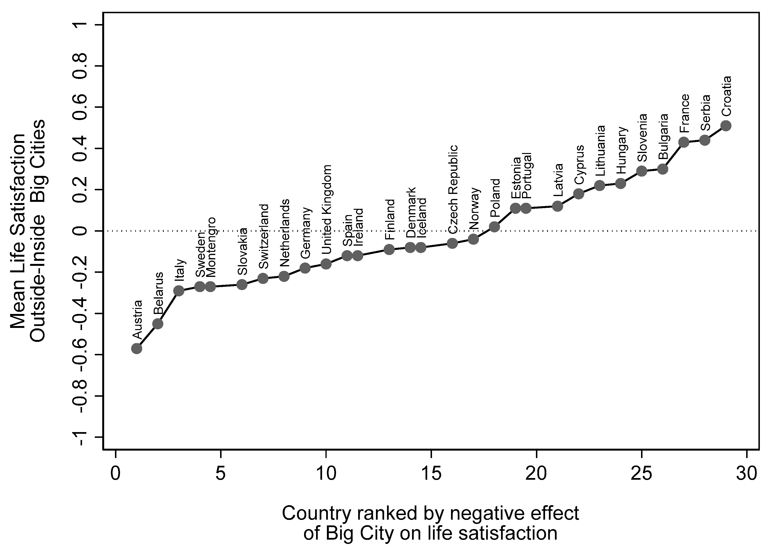
Figure 2.
The Functional Urban Area and NUTS2 classification of Austria. Source: [email protected]. January 2019, https://ec.europa.eu/eurostat/data/database. (Last accessed 29 September 2021).
Figure 2.
The Functional Urban Area and NUTS2 classification of Austria. Source: [email protected]. January 2019, https://ec.europa.eu/eurostat/data/database. (Last accessed 29 September 2021).
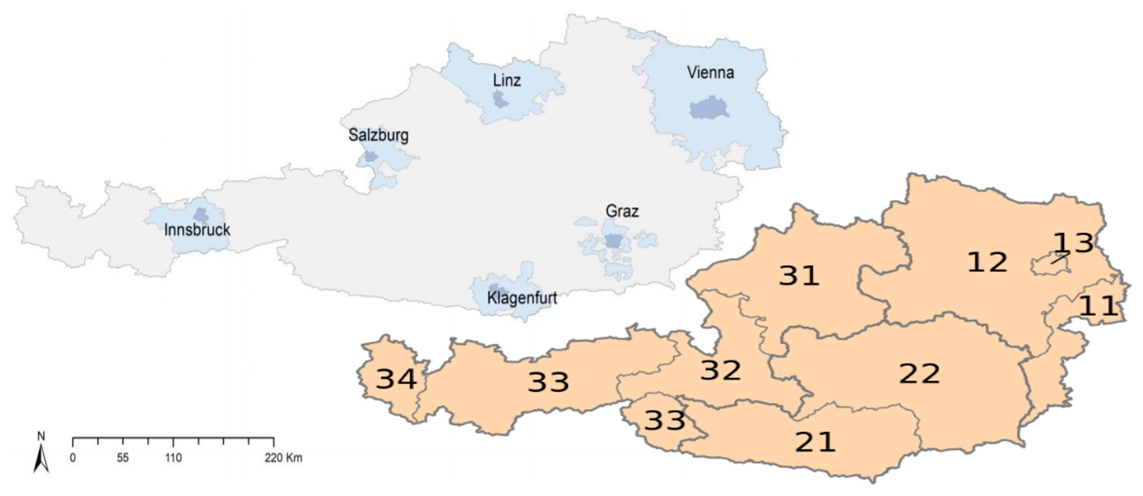
Figure 3.
The density and quantile plots of life satisfaction inside and outside the Vienna FUA. Austria, 2018. Source: ESS9. Note: The dotted vertical line in panel b identifies the bottom 10 percent of the life satisfaction distribution within the Vienna FUA. These approximately 97.3 (n = 0.10 × 973) individuals have a score of 5 or less on the 0 to 10 life satisfaction scale. The bottom ten percent living outside the Vienna FUA (n = 0.10 × 1526 = 152.6) have a score of just above 5.5 or less on the Y scale. The scores associated with the remaining quantiles can be read off the quantile plot accordingly.

Figure 4.
The differential influence of residence in the Vienna FUA at successive deciles of the life satisfaction and happiness. Austria, 2018. Source: ESS9.
Figure 4.
The differential influence of residence in the Vienna FUA at successive deciles of the life satisfaction and happiness. Austria, 2018. Source: ESS9.

Figure 5.
The differential influence of residence in the Prague and Ljubljana FUAs at successive deciles of life satisfaction and happiness. Czech Republic and Slovenia, 2018. Source: ESS9.
Figure 5.
The differential influence of residence in the Prague and Ljubljana FUAs at successive deciles of life satisfaction and happiness. Czech Republic and Slovenia, 2018. Source: ESS9.


Table 1.
Urbanisation in Europe. Countries surveyed in the European Social Survey in 2018 (ESS9) sorted by population size (‘000).
Table 1.
Urbanisation in Europe. Countries surveyed in the European Social Survey in 2018 (ESS9) sorted by population size (‘000).
| 1 | 2 | 3 | 4 | 5 |
|---|---|---|---|---|
| Country | Population | Urban | Rural | Percent urban |
| Germany | 82,293 | 63,622 | 18,671 | 77.3 |
| United Kingdom | 66,574 | 55,521 | 11,052 | 83.4 |
| France | 65,233 | 52,476 | 12,757 | 80.4 |
| Italy | 59,291 | 41,763 | 17,528 | 70.4 |
| Spain | 46,397 | 37,267 | 9130 | 80.3 |
| Poland | 38,105 | 22,885 | 15,220 | 60.1 |
| Netherlands | 17,084 | 15,631 | 1454 | 91.5 |
| Czech Republic | 10,625 | 7841 | 2785 | 73.8 |
| Portugal | 10,291 | 6711 | 3580 | 65.2 |
| Sweden | 9983 | 8728 | 1255 | 87.4 |
| Hungary | 9689 | 6913 | 2776 | 71.4 |
| Belarus | 9452 | 7429 | 2023 | 78.6 |
| Serbia | 8762 | 4915 | 3847 | 56.1 |
| Austria | 8752 | 5102 | 3650 | 58.3 |
| Switzerland | 8544 | 6305 | 2239 | 73.8 |
| Bulgaria | 7037 | 5278 | 1759 | 75.0 |
| Denmark | 5754 | 5057 | 698 | 87.9 |
| Finland | 5543 | 4732 | 810 | 85.4 |
| Slovakia | 5450 | 2928 | 2522 | 53.7 |
| Norway | 5353 | 4403 | 950 | 82.2 |
| Ireland | 4804 | 3035 | 1769 | 63.2 |
| Croatia | 4165 | 2372 | 1793 | 56.9 |
| Lithuania | 2876 | 1947 | 930 | 67.7 |
| Slovenia | 2081 | 1135 | 946 | 54.5 |
| Latvia | 1930 | 1315 | 615 | 68.1 |
| Estonia | 1307 | 900 | 407 | 68.9 |
| Cyprus | 1189 | 794 | 395 | 66.8 |
| Montenegro | 629 | 420 | 209 | 66.8 |
| Iceland | 338 | 317 | 21 | 93.8 |
Source: United Nations, Department of Economic and Social Affairs, Population Division (2018). World Urbanization Prospects: The 2018 Revision, Online Edition.
Table 2.
Grouped domicils of countries surveyed by the European Social Survey in 2018 (ESS9), sorted alphabetically.
Table 2.
Grouped domicils of countries surveyed by the European Social Survey in 2018 (ESS9), sorted alphabetically.
| 1 | 2 | 3 | 4 | 5 |
|---|---|---|---|---|
| Country | Big City & Suburbs | Small Town | Country & Farm | Total |
| Austria | 31.5 | 24.6 | 43.9 | 100 |
| Belarus | 23.0 | 26.9 | 50.1 | 100 |
| Bulgaria | 37.6 | 30.2 | 32.2 | 100 |
| Croatia | 38.0 | 25.4 | 36.6 | 100 |
| Cyprus | 53.7 | 15.0 | 31.4 | 100 |
| Czech Republic | 40.1 | 30.6 | 29.3 | 100 |
| Denmark | 40.8 | 31.1 | 28.1 | 100 |
| Estonia | 39.3 | 32.6 | 28.1 | 100 |
| Finland | 35.4 | 31.3 | 33.3 | 100 |
| France | 31.1 | 34.7 | 34.3 | 100 |
| Germany | 31.4 | 35.8 | 32.8 | 100 |
| Hungary | 25.7 | 36.9 | 37.4 | 100 |
| Iceland | 35.8 | 43.1 | 21.1 | 100 |
| Ireland | 31.8 | 27.1 | 41.1 | 100 |
| Italy | 18.4 | 34.7 | 47.0 | 100 |
| Latvia | 28.1 | 31.9 | 40.1 | 100 |
| Lithuania | 26.3 | 30.0 | 43.7 | 100 |
| Montenegro | 27.8 | 47.8 | 24.4 | 100 |
| Netherlands | 27.6 | 27.0 | 45.4 | 100 |
| Norway | 32.0 | 32.6 | 35.4 | 100 |
| Poland | 22.5 | 33.2 | 44.3 | 100 |
| Portugal | 37.6 | 35.2 | 27.2 | 100 |
| Serbia | 43.6 | 20.8 | 35.6 | 100 |
| Slovakia | 26.6 | 24.8 | 48.6 | 100 |
| Slovenia | 24.8 | 22.3 | 53.0 | 100 |
| Spain | 25.1 | 30.2 | 44.8 | 100 |
| Sweden | 39.3 | 33.4 | 27.3 | 100 |
| Switzerland | 17.6 | 27.4 | 55.0 | 100 |
| United Kingdom | 29.5 | 45.4 | 25.2 | 100 |
Source: ESS9. Note: Austria GDP/capita 2018 $58,851; Czech Republic $42,425, Slovenia $40,144.
Table 3.
Mean life satisfaction and happiness associations with five measures of agglomeration. Austria, 2018. (a) Life satisfaction, (b) Happiness.
Table 3.
Mean life satisfaction and happiness associations with five measures of agglomeration. Austria, 2018. (a) Life satisfaction, (b) Happiness.
| (a) | |||||
| Agglomeration (n) | (1) | (2) | (3) | (4) | (5) |
| Big City (571) | −0.52 *** | ||||
| (0.136) | |||||
| Big City and Suburbs (788) | −0.449 *** | ||||
| (0.122) | |||||
| ViennaCity (410) | −0.517 *** | ||||
| (0.157) | |||||
| ViennaSub (545) | −0.475 *** | ||||
| (0.146) | |||||
| ViennaFUA (973) | −0.461 *** | ||||
| (0.108) | |||||
| Constant | 8.05 *** | 8.074 *** | 8.023 *** | 8.042 *** | 8.108 *** |
| (0.053) | (0.056) | (0.052) | (0.053) | (0.063) | |
| Observations | 2495 | 2495 | 2495 | 2495 | 2495 |
| R-squared | 0.016 | 0.014 | 0.013 | 0.013 | 0.016 |
| (b) | |||||
| (1) | (2) | (3) | (4) | (5) | |
| Big City | −0.481 *** | ||||
| (0.103) | |||||
| Big City and Suburbs | −0.428 *** | ||||
| (0.094) | |||||
| ViennaCity | −0.538 *** | ||||
| (0.117) | |||||
| ViennaSub | −0.504 *** | ||||
| (0.107) | |||||
| ViennaFUA | −0.537 *** | ||||
| (0.086) | |||||
| Constant | 8.021 *** | 8.047 *** | 8.008 *** | 8.03 *** | 8.119 *** |
| (0.046) | (0.048) | (0.045) | (0.046) | (0.053) | |
| Observations | 2490 | 2490 | 2490 | 2490 | 2490 |
| R-squared | 0.016 | 0.015 | 0.017 | 0.018 | 0.026 |
Source: ESS9 estimated with sample weights. Standard errors are in parentheses. *** p < 0.01, ** p < 0.05, * p < 0.1.
Table 4.
Estimated sample means of the variables used in the models of subjective wellbeing. Austria, 2018.
Table 4.
Estimated sample means of the variables used in the models of subjective wellbeing. Austria, 2018.
| Variable | Obs | Mean | Std. Dev. | Min | Max |
|---|---|---|---|---|---|
| How satisfied with life as a whole? | 2495 | 7.92 | 1.79 | 0 | 10 |
| How happy would you say you are? | 2490 | 7.90 | 1.63 | 0 | 10 |
| Inside Vienna FUA | 2499 | 0.40 | 0.50 | 0 | 1 |
| Age-centered | 2489 | 0 | 18.71 | −36.56 | 38.44 |
| Female | 2499 | 0.52 | 0.51 | 0 | 1 |
| Born in country | 2499 | 0.85 | 0.35 | 0 | 1 |
| Unemployed | 2497 | 0.05 | 0.22 | 0 | 1 |
| In good health | 2499 | 0.77 | 0.42 | 0 | 1 |
| Tertiary qualification | 2494 | 0.24 | 0.43 | 0 | 1 |
| Coping on income | 2470 | 0.85 | 0.35 | 0 | 1 |
| Legally married | 2499 | 0.51 | 0.50 | 0 | 1 |
| Sociable | 2499 | 0.68 | 0.47 | 0 | 1 |
| Trusting | 2497 | 0.54 | 0.50 | 0 | 1 |
| Religious | 2499 | 0.43 | 0.49 | 0 | 1 |
| Safe at night | 2499 | 0.85 | 0.35 | 0 | 1 |
Source: ESS9. Survey weights applied. Note: The variable labelled unemployed has been coded to also include those who are permanently sick or disabled. In good health includes those in good and very good health. Coping on current income refers to those who said they were either coping or living comfortably on their present income. Sociable refers to those who meet socially with friends, relatives, or work colleagues once a week or more. Trusting refers to those who answer 6–10 on the 0–10-point scale with respect to the statement ‘most people can be trusted (or you can’t be too careful in dealing with people)’. Religious identifies those who score between 6 and 10 on the 0–10 scale in response to the statement ‘Regardless of whether you belong to a particular religion, how religious would you say you are?’. Safe at night refers to those who answer very safe or safe in response to the question ‘How safe do you—or would you—feel walking alone in this area after dark?
Table 5.
OLS estimates of association between agglomeration and life satisfaction and happiness. Austria, 2018. (a) Life satisfaction, (b) Happiness.
Table 5.
OLS estimates of association between agglomeration and life satisfaction and happiness. Austria, 2018. (a) Life satisfaction, (b) Happiness.
| (a) | |||||||
| (1) | (2) | (3) | (4) | (5) | (6) | (7) | |
| Vienna FUA | −0.461 *** | −0.437 *** | −0.394 *** | −0.373 *** | −0.352 *** | −0.395 *** | −0.378 *** |
| Age-centered | −0.003 | −0.005 ** | 0.005 ** | 0.004 * | 0.005 ** | 0.003 | |
| Female | 0.267 *** | 0.185 ** | 0.181 ** | 0.181 ** | 0.184 ** | 0.237 *** | |
| Born in country | 0.714 *** | 0.591 *** | 0.495 ** | 0.486 ** | 0.271 | 0.295 * | |
| Unemployed | −1.76 *** | −1.45 *** | −1.46 *** | −1.038 *** | −1.042 *** | ||
| In good health | 1.132 *** | 1.149 *** | 0.993 *** | 0.88 *** | |||
| Tertiary qualification | −0.169 | −0.172 | −0.242 ** | ||||
| Coping on income | 1.155 *** | 1.085 *** | |||||
| Legally married | 0.232 ** | ||||||
| Sociable | 0.39 *** | ||||||
| Trusting | 0.213 ** | ||||||
| Religious | 0.188 * | ||||||
| Safe at night | 0.404 *** | ||||||
| Constant | 8.108 *** | 7.355 *** | 7.574 *** | 6.765 *** | 6.793 *** | 6.091 *** | 5.275 *** |
| Observations | 2495 | 2485 | 2483 | 2483 | 2478 | 2451 | 2449 |
| R-squared | 0.016 | 0.042 | 0.087 | 0.149 | 0.15 | 0.196 | 0.225 |
| (b) | |||||||
| (1) | (2) | (3) | (4) | (5) | (6) | (7) | |
| Vienna FUA | −0.537 *** | −0.527 *** | −0.494 *** | −0.475 *** | −0.483 *** | −0.507 *** | −0.497 *** |
| Age-centered | −0.007 *** | −0.009 *** | 0 | 0 | 0 | −0.003 | |
| Female | 0.184 ** | 0.122 | 0.118 | 0.118 | 0.13 * | 0.184 ** | |
| Born in country | 0.429 *** | 0.339 ** | 0.247 | 0.252 | 0.11 | 0.146 | |
| Unemployed | −1.271 *** | −0.981 *** | −0.979 *** | −0.68 *** | −0.663 *** | ||
| In good health | 1.068 *** | 1.06 *** | 0.944 *** | 0.839 *** | |||
| Tertiary qualification | 0.06 | 0.039 | −0.026 | ||||
| Coping on income | 0.867 *** | 0.789 *** | |||||
| Legally married | 0.325 *** | ||||||
| Sociable | 0.277 *** | ||||||
| Trusting | 0.228 *** | ||||||
| Religious | 0.116 | ||||||
| Safe at night | 0.315 *** | ||||||
| Constant | 8.119 *** | 7.657 *** | 7.815 *** | 7.052 *** | 7.043 *** | 6.508 *** | 5.81 *** |
| Observations | 2490 | 2480 | 2478 | 2478 | 2474 | 2447 | 2445 |
| R-squared | 0.026 | 0.043 | 0.071 | 0.137 | 0.137 | 0.169 | 0.197 |
Source: ESS9. Survey weights applied. *** p < 0.01, ** p < 0.05, * p < 0.1.
Table 6.
Quantile regression of life satisfaction and happiness on the Vienna FUA and covariates. Estimates table. Austria, 2018. (a) Life satisfaction, (b) Happiness.
Table 6.
Quantile regression of life satisfaction and happiness on the Vienna FUA and covariates. Estimates table. Austria, 2018. (a) Life satisfaction, (b) Happiness.
| (a) | |||||||||||
| (1) | (2) | (3) | (4) | (5) | (6) | (7) | (8) | (9) | (10) | ||
| Q05 | Q10 | Q15 | Q20 | Q30 | Q40 | Q50 | Q60 | Q70 | Q80 | ||
| Vienna FUA | −0.137 | 0 | −0.25 * | −0.2 * | −0.325 *** | −0.335 *** | −0.379 *** | −0.35 *** | −0.349 *** | −0.66 *** | |
| Age-centered | 0.007 | 0 | 0 | 0 | 0.003 | 0.005 ** | 0.004 * | 0.004 | 0.007 *** | 0.005 * | |
| Female | 0.144 | 0 | 0.25 * | 0.2 * | 0.16 * | 0.194 *** | 0.135 * | 0.09 | 0.089 | 0.034 | |
| Born in country | 1.072 *** | 1 *** | 0.75 *** | 0.8 *** | 0.463 *** | 0.404 *** | 0.222 * | 0.188 | 0.171 | −0.107 | |
| Unemployed | −1.885 *** | −2 *** | −2 *** | −1.8 *** | −1.859 *** | −1.281 *** | −1.292 *** | −0.806 *** | −0.664 *** | −0.65 *** | |
| In good health | 1.777 *** | 1.5 *** | 1.25 *** | 1 *** | 0.887 *** | 0.755 *** | 0.752 *** | 0.746 *** | 0.774 *** | 0.835 *** | |
| Tertiary qual. | −0.482 | −0.5 ** | −0.25 | −0.2 | −0.12 | −0.122 | −0.057 | −0.104 | −0.116 | −0.063 | |
| Coping on income | 1.921 *** | 2 *** | 1.25 *** | 1.2 *** | 1.043 *** | 0.773 *** | 0.664 *** | 0.692 *** | 0.664 *** | 0.524 *** | |
| Legally married | 0.691 *** | 0.5 *** | 0.5 *** | 0.4 *** | 0.362 *** | 0.326 *** | 0.301 *** | 0.202 ** | 0.24 *** | 0.126 | |
| Sociable | 0.468 * | 0.5 *** | 0.25 * | 0.4 *** | 0.445 *** | 0.435 *** | 0.412 *** | 0.336 *** | 0.288 *** | 0.223 ** | |
| Trusting | 0.763 *** | 0.5 *** | 0.5 *** | 0.6 *** | 0.368 *** | 0.262 *** | 0.139 * | 0.152 * | 0.068 | −0.019 | |
| Religious | 0.453 * | 0.5 *** | 0.25 * | 0.2 * | 0.209 ** | 0.181 ** | 0.17 ** | 0.158 * | 0.171 ** | 0.073 | |
| Safe at night | 0.705 ** | 1 *** | 0.75 *** | 0.6 *** | 0.347 *** | 0.373 *** | 0.364 *** | 0.304 *** | 0.301 *** | 0.092 | |
| Constant | −0.467 | 0.5 | 2.5 *** | 3 *** | 4.381 *** | 5.181 *** | 5.924 *** | 6.452 *** | 6.912 *** | 8.224 *** | |
| Observations | 2449 | 2449 | 2449 | 2449 | 2449 | 2449 | 2449 | 2449 | 2449 | 2449 | |
| (b) | |||||||||||
| (1) | (2) | (3) | (4) | (5) | (6) | (7) | (8) | (9) | (10) | ||
| Q05 | Q10 | Q15 | Q20 | Q30 | Q40 | Q50 | Q60 | Q70 | Q80 | ||
| Vienna FUA | −0.03 | −0.401 *** | −0.388 *** | −0.399 *** | −0.433 *** | −0.449 *** | −0.462 *** | −0.512 *** | −0.294 *** | −0.75 *** | |
| Age-centered | −0.007 | −0.002 | −0.003 | −0.003 | −0.002 | −0.004 * | −0.005 ** | −0.004 ** | −0.001 | 0 | |
| Female | 0.104 | 0.176 | 0.103 | 0.095 | 0.064 | 0.218 *** | 0.131 ** | 0.139 * | 0.097 | 0 | |
| Born in country | 0.785 ** | 0.555 ** | 0.649 *** | 0.559 *** | 0.242 * | 0.308 *** | −0.025 | −0.083 | −0.157 | 0 | |
| Unemployed | −0.993 ** | −0.826 ** | −1.083 *** | −1.327 *** | −1.195 *** | −0.811 *** | −0.882 *** | −0.754 *** | −0.453 ** | −0.25 | |
| In good health | 1.407 *** | 1.434 *** | 1.259 *** | 1.137 *** | 0.879 *** | 0.697 *** | 0.686 *** | 0.735 *** | 0.787 *** | 0.75 *** | |
| Tertiary qual | 0.052 | 0.178 | 0.149 | 0.114 | 0.032 | 0.064 | 0.063 | −0.01 | −0.02 | 0 | |
| Coping on income | 1.393 *** | 1.247 *** | 1.037 *** | 0.846 *** | 0.934 *** | 0.5 *** | 0.467 *** | 0.426 *** | 0.403 *** | 0.5 *** | |
| Legally married | 0.741 *** | 0.718 *** | 0.615 *** | 0.549 *** | 0.476 *** | 0.467 *** | 0.435 *** | 0.353 *** | 0.244 *** | 0.25 *** | |
| Sociable | 0.244 | 0.441 *** | 0.388 *** | 0.376 *** | 0.448 *** | 0.397 *** | 0.327 *** | 0.242 *** | 0.179 ** | 0.25 *** | |
| Trusting | 0.726 *** | 0.634 *** | 0.532 *** | 0.467 *** | 0.417 *** | 0.325 *** | 0.209 *** | 0.11 | 0.088 | 0 | |
| Religious | 0.674 *** | 0.39 *** | 0.244 ** | 0.35 *** | 0.087 | 0.178 ** | 0.133 * | 0.168 ** | 0.083 | 0 | |
| Safe at night | 0.704 ** | 0.529 *** | 0.471 *** | 0.552 *** | 0.218 ** | 0.387 *** | 0.452 *** | 0.436 *** | 0.394 *** | 0.25 ** | |
| Constant | 0.562 | 1.85 *** | 2.799 *** | 3.447 *** | 4.744 *** | 5.422 *** | 6.231 *** | 6.77 *** | 7.28 *** | 8 *** | |
| Observations | 2445 | 2445 | 2445 | 2445 | 2445 | 2445 | 2445 | 2445 | 2445 | 2445 | |
Source: ESS9. *** p < 0.01, ** p < 0.05, * p < 0.1.
Publisher’s Note: MDPI stays neutral with regard to jurisdictional claims in published maps and institutional affiliations. |
© 2021 by the author. Licensee MDPI, Basel, Switzerland. This article is an open access article distributed under the terms and conditions of the Creative Commons Attribution (CC BY) license (https://creativecommons.org/licenses/by/4.0/).
Share and Cite
MDPI and ACS Style
Morrison, P.S. Whose Happiness in Which Cities? A Quantile Approach. Sustainability 2021, 13, 11290. https://doi.org/10.3390/su132011290
AMA Style
Morrison PS. Whose Happiness in Which Cities? A Quantile Approach. Sustainability. 2021; 13(20):11290. https://doi.org/10.3390/su132011290
Chicago/Turabian StyleMorrison, Philip S. 2021. "Whose Happiness in Which Cities? A Quantile Approach" Sustainability 13, no. 20: 11290. https://doi.org/10.3390/su132011290
Note that from the first issue of 2016, this journal uses article numbers instead of page numbers. See further details here.