
Is Inflation Fiscally Determined?


Graduate School of Economics and Management, Tohoku University, Sendai 980-8576, Japan
*
Author to whom correspondence should be addressed.
Sustainability 2021, 13(20), 11306; https://doi.org/10.3390/su132011306
Submission received: 24 August 2021
/
Revised: 1 October 2021
/
Accepted: 4 October 2021
/
Published: 13 October 2021
(This article belongs to the Special Issue Fiscal Policy, the Theory and its Role in a Future Sustainable Economy Development)
Abstract
:This paper examines the relationship between fiscal policy and inflation for 44 countries, from 1960 to 2020. The study was conducted using a panel VAR approach while accounting for the difference in monetary policy frameworks and the levels of fiscal space across countries. Results suggest that budget deficits are less likely to cause inflation when monetary policy is based on inflation targeting. In contrast, they are inflationary in the group of countries with a poorly structured monetary policy (such as partially dollarized Latin American economies).
1. Introduction
In recent decades, many countries have attempted to bolster weak economic growth using fiscal policy. The resulting increase in public debt, macroeconomic imbalances, and, more particularly, effects on price levels are now a source of public concern. Nonetheless, the fears surrounding a burst of inflation resulting from high indebtedness is justifiable only if a verifiable relationship between inflation and fiscal policy exists.
The literature usually links inflation to monetary policy factors. For example, the monetarist view suggests that inflation is the result of too much money, chasing too few goods, and often emphasizes the importance of the demand for money, interest rates, and exchange rates. In general, the conduct of monetary policy is usually considered to be a major determinant of inflation dynamics and the primary explanation for the recent low levels of inflation. Fiscal determinacy of the price level, on the other hand, is based on the idea that governments running persistent deficits will eventually have to finance those deficits by creating money (seigniorage), thus producing higher inflation, especially when the GDP growth rate is below the interest rate (Sargent and Wallace [1]). The most popular works in this respect are those on the fiscal theory of the price level (FTPL). Nevertheless, prior empirical studies find little success in uncovering strong evidence for its validity or in deriving consistent results across advanced and developing economies.
We believe that the absence of conclusive empirical evidence in this area is partly because such studies rarely control the effects of monetary policy. The main hypothesis in this paper is that inflation is more likely to respond to fiscal policy measures when monetary policy is based on approaches that coincide with regimes of passive monetary policy/active fiscal policy. It is therefore important to account for the difference in monetary policy frameworks across periods and countries. In addition, we also attempt to explain why a closer relationship between inflation and fiscal deficits is more often seen in developing (rather than advanced) economies. We assume that this contrast could be explained by different debt repayment capacities and also control for this factor by including a measure of fiscal space in the analysis.
Based on a linearized equation derived from a government’s intertemporal budget constraint, the present study employs a panel vector auto-regression (PVAR) model to analyze a sample of 44 countries over the period 1960–2020. The panel approach presents several advantages over the more traditional country-by-country analysis. First, it provides estimates that reflect the common behavior of the sample while controlling for individual heterogeneity. Therefore, it offers a more general conclusion from the analysis than would be possible from a time-series approach. Second, the additional cross-sectional dimension allows for a gain in degrees of freedom (compared to time-series). Finally, the greater variability that characterizes panel data improves the efficiency of econometric estimates.
Our underlying theoretical model links the inflation rate to both fiscal and monetary policy variables, in addition to economic growth rates. Adopting both restricted and unrestricted PVAR approaches in the estimation, we analyze the changes in the response of inflation to fiscal variables based on the category of the monetary policy framework. The main findings indicate that fiscal variables are less likely to affect inflation when monetary policy is based on targets. In particular, inflation is less responsive to fiscal shocks (and interest rates shocks) in inflation targeting regimes. On the other hand, budget deficits are inflationary for the category of countries with a poorly structured monetary policy (such as partially dollarized Latin American countries). Finally, as opposed to monetary policy, the fiscal space level does not play a significant role in explaining the relationship between fiscal policy and inflation.
2. Literature Review
There are three broad approaches to link fiscal policy with inflation. The traditional approach is based on the government budget constraint, used first by Sargent and Wallace [1] to establish the link between fiscal policy and the price level. They derive the fiscal determinacy of prices from the government’s intertemporal budget constraint, expressed as
where is government expenditures on goods, services, and transfers at time t, is the tax revenue, is the interest rate, is interest-bearing debt, and is the stock of base or high-powered money. Thus, represents interest payments on total outstanding debt and denotes new issues of interest-bearing debt. Equation (1) shows that the government can fund its expenditures either through taxes, newly issued debt, or printing new currency ().
Based on Equation (1), Sargent and Wallace [1] provide an expression for the inflation rate that depends on the stock of interest-bearing government debt per capita, assuming that fiscal policy dominates monetary policy. That is, the fiscal authority sets its budget independently, announcing the current and future deficits and surpluses. The amount of revenue to raise is then determined based on these decisions. The monetary authority then finances the discrepancy between the revenue demanded by the fiscal authority and the number of bonds it can sell to the public with seigniorage. Leeper [2] defines this as an “active” fiscal policy and “passive” monetary policy scenario, where the fiscal authority’s actions constrain monetary policy, which simply reacts to government debt shocks. An important idea in this model is that, if the interest rates on bonds are higher than the economy’s growth rate, then the real stock of bonds will grow faster than the economy. However, as the demand for bonds places an upper limit on the stock of bonds, the government will eventually finance both the principal and the interest through seigniorage. In other words, the fiscal authority’s decisions can induce the printing of more money, and therefore inflation.
Most existing empirical studies on the fiscal determinacy of the price level use the government’s intertemporal budget constraint as the starting point to determine both the analytical approach and the explanatory variables. Some of these studies focus on the link between fiscal deficits and inflation, while others examine the relationship between fiscal surpluses and public debt, or use a different approach (see Table 1). However, most studies do not provide conclusive evidence for the existence of the fiscal determinacy of prices. For example, Catao and Terrones [3] and Fischer, Sahay and Végh [4] conclude that fiscal deficits are the main drivers of high inflation only for high-inflation developing countries. Bohn [5] and Bajo-Rubio, Díaz-Roldán and Esteve [6] follow a different approach, using the primary surplus and the debt-to-GDP ratio. Bajo-Rubio, Díaz-Roldán and Esteve [6] examine a sample of 11 EU countries, while Bohn [5] studies only the US. They conclude that the fiscal authority acts in a Ricardian fashion, as do Canzoneri, Cumby and Diba [7] and Creel and Le Bihan [8]. According to Sargent [9] (pp. 6–7), in a Ricardian regime, the issuing of additional interest-bearing government securities is always accompanied by a planned increase in explicit future tax collections, which is sufficient to repay the debt. In the second polar regime (non-Ricardian), additional interest-bearing government securities signify the government’s promise to eventually monetize the interest-bearing debt. In contrast to the aforementioned literature, Favero and Monacelli [10] show the presence of alternating Ricardian and non-Ricardian regimes.
A distinct strand in the theoretical literature, known as the FTPL, emerged based on the assumption of a dominant fiscal policy. The central equation of the FTPL is the government debt valuation equation, which sets the real value of government debt equal to the expected present value of future fiscal surpluses.
where is the one-period nominal debt issued at due at t, is the price level, is the real primary government surplus including seigniorage, and is the discount factor. Several papers provide derivations of this equation, such as Sims [11] and Woodford [12], Woodford [13]. The valuation equation is usually obtained from the intertemporal government budget constraint, with the government debt ( on the LHS) expressed in nominal terms and the present value of primary surpluses (RHS) in real terms. Cochrane [14] presents this relation as an asset pricing model based on a different logic. The underlying idea is that nominal debt, including the monetary base, is a claim on the government’s future primary surpluses (as a stock is a claim on future earnings). As the author argues, the market determines bond prices depending on bond yields and future streams of expected primary surpluses Cochrane [15].
Estimating Equation (2) provides a direct verification of the FTPL. However, this approach poses many challenges. First, the variable representing the present value of future primary surpluses would be hard to measure and analyze. Second, the choice of the discount rate would have a significant impact on the results. A change in inflation could reflect a change in the discount rate rather than a movement in fiscal variables (Cochrane [16]). Furthermore, inferring concrete policy implications from this formal expression is not straightforward. However, using a similar expression with alternative empirical approaches, some studies were able to confirm the validity of the FTPL (e.g., Loyo [17] and Tanner and Ramos [18] for Brazil or Fan and Minford [19] for the UK).
Another limit of the government’s valuation equation is the fact that it omits many important economic variables that play key roles in inflation dynamics. One example is the economic growth rate. As Sargent and Wallace [1] point out, the fiscal determinacy of prices occurs when the economic growth rate is below the interest rate. This condition cannot be verified through the valuation equation. Therefore, there is a need for a more comprehensive theoretical framework that incorporates assumptions that align more closely with actual economic dynamics.
Sims [20] suggests such a framework. It is a new-Keynesian-style model with long-term debt and sticky prices. One important implication of this model is that even in an active fiscal/passive monetary policy equilibrium, the monetary variables still have a powerful effect on both output and inflation. As discussed by Cochrane [15], the fiscal determinacy mechanism takes place in this framework through the transmission channel of bond prices. More precisely, when monetary policy produces high interest rates, the real value of government debt appears to be greater than its real market value for investors. Consequently, the demand for government debt increases at the expense of the demand for goods and services, which leads to lower aggregate demand, and thereby to lower prices.
More recently, Cochrane [21] studied the fiscal roots of inflation based on the following log linearized identity
where represents the market value of debt, is the nominal returns on the government debt portfolio with a maturity length of n, is the inflation rate, is GDP growth, is the real primary surplus, and is the discount rate for the terms on the RHS. An expression derived from this identity (see Appendix A) shows that unexpected inflation that is less than the unexpected nominal return on government bonds must equal the innovation in the present value of future surpluses to GDP. Therefore, it links the unexpected inflation rate to both the monetary and fiscal variables, in addition to GDP growth (included in the discount rate of the present value). Using US data on government bonds from Hall, Payne and Sargent [22]’s database, Cochrane reports that a positive monetary policy shock (defined as a shock to interest rates not accompanied by a movement in future primary surpluses) is super-Fisherian and raises inflation immediately. A negative fiscal shock (defined as a shock to future primary surpluses not accompanied by a movement in interest rates) induces protracted inflation. The disinflation resulting from a recessionary shock corresponds entirely to a decline in discount rates, leading to higher debt. In our study, we apply a similar approach based on different assumptions using panel data for 44 countries for the sample period 1960–2020. We also attempt to compare the findings across subsamples constructed based on monetary policy frameworks and the level of fiscal space.

Table 1.
Some empirical studies on the fiscal determinacy of the price level.
| Paper | Sample | Methodology | Conclusion |
|---|---|---|---|
| Catao and Terrones [3] | 107 countries over 1960–2001 | ARDL model | Inflation and fiscal deficits are only correlated in the case of high-inflation, developing economies |
| Bohn [5] | US data 1916–1995 | OLS regressions by periods and a non-linear model for PB (based on debt) | The fiscal authority acts in a Ricardian fashion (Primary Balance adjusts) |
| Bajo-Rubio et al. [6] | 11 EU countries 1970–2005 | Cointegration analysis, Granger causality tests | Weak evidence for FTPL (Ricardian or monetary dominant regime) |
| Canzoneri et al. [7] | postwar U.S. data 1951–1995 | VAR, IRF | Evidence of a Ricardian regime |
| Favero and Monacelli [10] | US 1960–2002 | Markov-switching regression methods | Alternated Ricardian and non-Ricardian regime |
| Tanner and Ramos [18] | Brazil 1991–2000 | VAR, IRF, and Granger causality tests | Fiscal dominance for the case of Brazil for some important periods |
| Creel and Le Bihan [8] | France, Germany, Italy, the UK, and the US data 1963–2001 | VAR, IRF (same approach as [7]), and separation between structural/cyclical PB | FTPL non-valid |
| Fan and Minford [19] | The UK in the 1970s | ARIMA model for inflation, ADF, and cointegration tests | Behavior of inflation can be explained by the FTPL (government expenditures) |
3. Theoretical Model
We follow Cochrane [21] in deriving a model of inflation that accounts for the effect of fiscal policy, in addition to two important determinants of inflation in theory: monetary policy (through the interest rate) and aggregate demand (through GDP growth). Nonetheless, we base our model on the intertemporal government budget constraint rather than using an asset pricing approach. In addition, we consider the stock of government debt instead of the market value of bonds (it is more challenging to empirically verify a model that includes bond prices for different maturities in a panel study due to the lack of data). Finally, we do not include money in the variable of government debt as this may generate a bias when studying the relationship between debt and inflation.
The model is derived from the following government intertemporal budget constraint:
where denotes the stock of government debt in nominal terms at time t, the nominal interest rate on government bonds, nominal government spending, and taxes. This relation states that the government finances its spending and interest payments through taxes or by issuing new debt. We can express the percent change in the value of the government bond portfolio by h such that . Then, Equation (4) becomes
where is the primary surplus at time t. The primary surplus is defined as the difference between government revenues and government expenditures, excluding interest payments. Since the change in public debt also depends on government bond yields, we assume that it can be expressed as a linear function of this variable, such that for a given coefficient k (). Then, we can write Equation (5) as
with being GDP growth, and rescaling by real GDP leads to
where and represent the terms and rescaled by GDP, respectively. This relation is equivalent to
Dividing this equation by yields
With inflation corresponding to and the output-adjusted real primary surplus being , we get
Considering real debt over GDP (= ),
Taking the logs and bringing inflation to the LHS, we obtain
In this equation, it appears that both fiscal and monetary policy, in addition to growth, affect the inflation level. Based on this model, we expect a positive relationship between inflation and public debt and a negative relationship between inflation and the primary balance. Moreover, we assume that inflation will have a positive response to interest rates. These expectations are consistent with the neo-Fisherian principle.
In addition, we expect a negative relationship between inflation and the GDP growth rate. This result contradicts the conventional Keynesian and neo-Keynesian frameworks, according to which this relation should be positive (the AD–AS model, Phillips Curve). However, this assumption is consistent with findings from several empirical studies and theoretical models. For example, Stockman [23] establishes that an increase in the inflation rate results in a lower steady-state output level by reducing the purchasing power of money balances and, thus, the demand for goods and capital (this model assumes that part of the investment project is financed through cash). Similarly, most money and endogenous growth models conclude that the inflation rate reduces both the return on capital and the growth rate in the long run (Arawatari, Hori and Mino [24], Vaona [25]). Empirically, several studies reveal an overall negative effect of inflation on growth and detect that this relationship is non-linear (e.g., Andres and Hernando [26], De Gregorio [27], Fischer [28], Gomme [29], Kormendi and Meguire [30]).
4. Data and Approach
Unlike previous studies that focus on a single country, we study the inflation-fiscal variables relationship using a PVAR model over a long period to draw more general conclusions. Equation (12) contains the key variables required for the analysis. We examine their relationship using a sample of 44 countries, from 1960 to 2020, selected based on data availability. The sample countries are listed in Appendix B and the data sources are defined in Appendix C. Yearly evolution of data shows that the level of indebtedness has overall been increasing over the recent years, especially in advanced economies. On the other hand, inflation levels became very low for all countries after 1995. Over the period of study, the highest inflation values are those of the 1970s for advanced economies and the 1980s or the beginning of the 1990s for emerging and developing economies.
From the evolution of primary balances of countries over the sample period, the following conclusions can be drawn. Countries with primary surpluses over most of the studied period include Norway, Denmark, Finland, Canada, and Switzerland. Some other countries only had surpluses over a limited time span; e.g., Mexico (1983–1997) and Chile (1987–1997, 2003–2008). Countries with long periods of deficits include Italy, Portugal, India, and Pakistan. In addition, the primary balance of all sample countries deteriorated after the 2008 crisis, and even more substantially after the COVID-19 outbreak.
Explanations for primary surpluses vary depending on countries and can be either due to the conduct of fiscal policy or to conjunctural factors. For instance, in the case of Norway, revenues from petroleum activities and the Government Pension Fund Global (GPFG) play an important role in balancing the government’s budget. In the case of Mexico, the improvement of the primary balance (that excludes debt servicing) in 1983 is mainly the result of both the debt restructuring program put in place after the 1982 debt crisis and the increase in oil output following heavy investments in this sector at the end of 1970s. On the other hand, the primary surplus of Chile in the 1990s can be explained by the prudent management of fiscal policy, high economic growth and privatization measures. The country’s finances were then significantly affected by the Asian crisis of 1997–1999. After 2003, the increase of surpluses reflects the success of the structural balance policy adopted by the country in 2000, based on the principle of setting a structural surplus goal (excluding temporary impacts of fluctuations in the business cycle and prices of commodities).
We further use the monetary policy classification compiled by Cobham [31] and data related to government revenues to determine the fiscal space level for the sample countries, as we explain in this section. The importance of accounting for monetary policy frameworks is justified by the common belief that the 1990s shift in monetary policy thinking by setting up rules or targets (money, credit, exchange rates, interest rates, and inflation) played a major role in controlling the inflation rate and addressing the dynamic inconsistency issue. A consensus in this literature is that commitment is a better policy because it generates lower average inflation in the long run (Barro and Gordon [32], Rogoff [33]). The gains from commitment are the direct consequence of the role of expectations in shaping economic conditions. More specifically, inflation targeting regimes are thought to contribute to lower inflation levels and higher monetary policy credibility.
We verify this assumption by applying Cobham [31]’s MPF classification to the sample. Cobham [31] defines an MPF as a combination of objectives, constraints, and conventions for monetary authorities. He distinguishes between different frameworks based on whether the monetary authorities publish targets for some objectives and whether such targets exist for monetary aggregates, exchange rates, inflation, and other variables. In this fashion, he identifies 32 different monetary policy frameworks, aggregated into 9 broad categories. Based on this classification and some slight adjustments, the dataset has been subdivided into the following groups:
- Exchange rate targets: the monetary authority intervenes to maintain the exchange rate at a particular level.
- Inflation targeting: this strategy relies on the use of inflation expectations to control the price level. It involves the announcement of numerical targets, accompanied by an institutional commitment to achieve these targets. Credibility and accountability of the monetary authority in that case are crucial to the conduct of monetary policy.
- Monetary targets: the monetary authority uses its instruments to achieve a target growth rate for a monetary aggregate that becomes the nominal anchor or intermediate target of monetary policy.
- Mixed targets: the monetary authority uses monetary targets and exchange rate fixes or targets, or three full targets (or fixes) (money, exchange rates, and inflation).
- Euro zone countries: Euro zone countries have been isolated in a separate group.
- Discretion: in that case, monetary policy is based on the ad hoc judgment of policymakers as opposed to the use of predetermined rules. The degree of effectiveness and coherence of the set of objectives and instruments in this case depends on the countries and periods. Moreover, most of the countries included in this category either do not have a significant use of foreign currency among residents or have substantially reduced this usage over the studied period.
- Poorly structured monetary policy: in this group, we isolate the countries characterized by a significant dollarization of the economy, and which either have no monetary policy framework (e.g., Panama) or use a poorly effective set of instruments or an incoherent mix of objectives over most of the sample period.
Data are available only for the period between 1980 and 2016. We therefore reduce the sample to this duration when including the MPF classification. The adjustments made to the classification of Cobham [31] are as follows: first the Euro zone countries classified in the group “No national framework” in Cobham [31] have been isolated in a separate group. Then fully dollarized economies (two countries classified in the group of “No national framework” in Cobham [31]) have been combined with highly dollarized economies with a poorly effective monetary policy (classified in the group of “unstructured discretion” in Cobham [31]) to form the group of “Poorly structured monetary policy”. By introducing the MPF classification, we assume that monetary policy would be considered as the main driver of inflation if the relationship between inflation and fiscal variables varies depending on the chosen framework. In that case, the relationship between fiscal policy and inflation would not be constant, but would depend on the strength of the relationship between monetary policy and inflation (case of an “active” monetary policy/“passive” fiscal policy).
An additional reason to account for the choice of MPFs is the fact that it affects the choice of the exchange rate regime, since the Mundell–Fleming trilemma implies the existence of a relationship between both decisions. For instance, countries with independent monetary authorities and open financial markets cannot opt for a fixed exchange rate regime. Similarly, more passive monetary policy frameworks are adopted in economies with exchange rate regimes based on “hard pegs”. As a result, the exchange rate pass-through to the price level may also vary depending on the MPFs. Generally, in the literature, pass-throughs are found to be lower in flexible exchange rate regimes (more commonly associated with the inflation targeting framework) (Ha, Stocker and Yilmazkuday [34]). Therefore, the choice of the MPF and its impact on exchange rate fluctuations could also affect inflation’s sensitivity to shocks.
In addition to MPFs, we also classify the sample countries by their fiscal space level (see definition in Heller [35]). We consider fiscal space to be an important factor because higher deficits are more likely to cause macroeconomic imbalances and disturbances in the price level when countries have a limited capacity to repay their debt and ensure sovereign solvency. The literature on fiscal space introduces many different measures. One frequent method is the “fiscal gap” approach, which is based on the difference between a given level of public debt or fiscal balance and a benchmark level considered as the sustainable level. Other studies (e.g., Auerbach and Gale [36], Buiter [37], Buiter, Corsetti and Roubini [38]) derive an index of fiscal sustainability based on the projections of future balances depending on the macroeconomic outlook and forecasts of the discount rate.
Aizenman and Jinjarak [39] suggest an alternative fiscal space measure called the “de facto fiscal space,” defined as the inverse of the number of tax-years needed to repay the debt. This ratio requires an estimate of the de facto tax base corresponding to the realized tax collection averaged across multiple years to smooth for business cycle fluctuations. We use a similar definition in this study. First, we calculate the ratio of public debt divided by total government revenues. This ratio reflects the number of years of revenue needed to repay the outstanding public debt on a given date. Then, we define fiscal space as the inverse of that ratio.
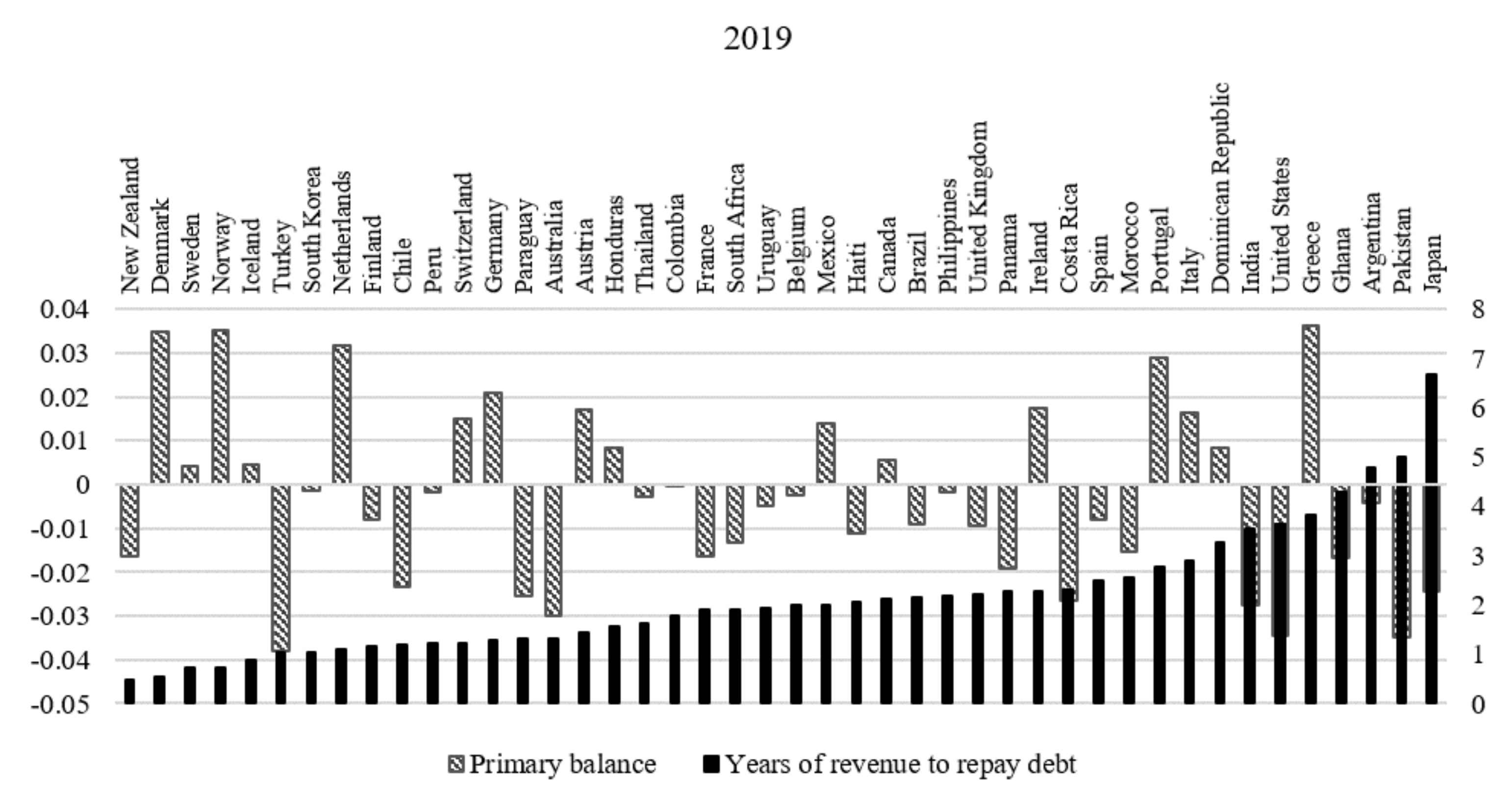
The data show the notable impact of the 2020 pandemic on fiscal space levels worldwide (Appendix D). In most countries, and especially in emerging economies, this impact is more significant than the one that resulted from fiscal stimulus measures implemented after the 2007 crisis. It should be noted that the lowest fiscal space measures for a given year do not necessarily coincide with the worst budget deficits. As shown in the Figure 1 below, both groups of countries running substantial budget deficits and those with high surpluses can have either low or high fiscal space levels. Appendix E shows the correlation coefficients between the primary balance and the inverse of the fiscal space ratio by country for different periods of time. This correlation varies over the sample period for each country. Still, we note that it tends to be more often negative and high in the recent two decades. This means that cases of countries with both high deficits and low fiscal space levels are more frequent in the recent period.
5. Econometric Methodology
After a correlation analysis (see following section), we estimate a PVAR model using the variables of Equation (12). The PVAR model is
where
and ,
where denotes the primary surplus over GDP, the log of public debt over GDP, the GDP growth rate, i the short-term interest rate, and the inflation rate. As we estimate the model based on panel data, we can interpret the vectors and as the stacked version of vectors and , respectively, where the index i indicates the different cross-sections (sample countries).
PVAR models are built on the same logic as standard time-series VARs and can be estimated using similar methods. However, they offer some key advantages over a time-series approach. First, PVAR models rely on the assumption that the cross-sectional units share the same underlying data generating process with common parameters across units. Thus, the obtained estimates reflect the common behavior of the group while controlling for individual heterogeneity. Second, the additional cross-sectional dimension is beneficial because it increases the degrees of freedom. In addition, panel data are characterized by a greater variability than time-series. Further, this variability improves the prospects of obtaining accurate estimates and the model is more likely to efficiently capture the relationships between macroeconomic variables.
The estimation of standard vector auto-regression (VAR) models in their reduced-form can be straightforwardly performed through ordinary least squares (OLS). However, the interpretation of the estimation results would be biased if the variables are correlated with each other (as is typically the case in macroeconomic models). Such correlation creates a dependence between the error terms across equations. Many techniques were developed to overcome this identification problem. One of them is the recursive VAR approach, and we apply this approach in the first step using a Cholesky decomposition of the covariance matrix, based on an active fiscal policy/passive monetary policy setting. The following ordering of the variables is used: the primary balance over GDP (most exogenous), public debt over GDP, GDP growth rate, short-term interest rates, and inflation (as in Equation (13)). We adopt this ordering because if fiscal policy is active, then the fiscal variables would be the most exogenous, and the short-term interest rate would, on the contrary, be more endogenous. In this setting, we expect that the dynamics affecting both the fiscal and monetary variables would lead to inflation fluctuations. We analyze this recursive VAR model based on variance decomposition.
Despite the advantages of the recursive approach, it is subject to the ordering problem. The chosen ordering determines which variables are contemporaneously unaffected by which other variables and it may not always be accurate. Therefore, we use other methods that address the endogeneity issue without relying on the recursive VAR restrictions. We first re-estimate the PVAR model based on the generalized method of moments (GMM) methodology suggested by Sigmund and Ferstl [40]. This approach is particularly useful to eliminate the Nickell bias (Nickell [41]) that arises when the demeaning process, which subtracts the individual’s mean values from the respective variables, induces a correlation between the error terms and regressors, thereby leading to inconsistent OLS estimates. Sigmund and Ferstl [40] provide an extension to Anderson and Hsiao [42] for the first-difference GMM estimator (also see Arellano and Bond [43], Holtz-Eakin, Newey and Rosen [44]) and also to the system GMM estimator of Blundell and Bond [45]. In the present paper, the first-difference GMM estimator is calculated for the model using one-period lags of the endogenous variables as instruments.
We analyze this unrestricted VAR model using generalized impulse response functions (GIRFs), as suggested by Pesaran and Shin [46]. The main advantage of this approach is that the response functions are not sensitive to the ordering of variables in the VAR model. In contrast to orthogonalized impulse response functions, the GIRF are unique and fully account for the historical patterns of correlations observed among the different shocks. However, because GIRFs provide only a statistical interpretation of the shocks and violate the assumptions required to analyze causal relationships (Kilian and Lütkepohl [47]), we choose to rely on both the restricted and unrestricted VAR approaches in order to ensure robustness.
6. Correlation Analysis
Table 2 reports the correlation coefficients between the main variables of the model for the whole sample. Interest rates and inflation have the highest correlation, which is positive (66%). Moreover, the inflation rate has weak correlations with the fiscal variables, while GDP growth is negatively correlated with public debt and positively with the primary balance.
These correlation coefficients differ significantly across monetary policy frameworks (Table 3). The highest correlation coefficient between inflation and the primary balance is 23% in the case of discretionary regimes. This category also shows the strongest correlation coefficient between inflation and interest rates (88%). In both cases, the relationship is positive. We see a negative relationship between the primary balance and inflation only in three cases: poorly structured monetary policy, mixed targets, and monetary targets. As opposed to other categories, regimes of mixed targets and monetary targets contain only a few observations (the mixed targets category applies to a few years in the 1980s for three countries (France, Germany, and Italy), while monetary targets apply to seven countries during the 1980s and the beginning of the 1990s). Finally, in the case of Euro zone countries, the correlation between inflation and interest rates is very high and positive, while the correlation between inflation and the primary balance is very low.
We then split the sample into two fiscal space categories based on the middle quantile. S1 is the subsample of higher fiscal space countries that require few years to repay their debt and S2 is the subsample of economies with lower fiscal space, which require many years to repay their debt. Table 4 provides the correlation coefficients for these two categories. The correlation coefficients between inflation and both the primary balance and public debt are very small for both subsamples. Conversely, the correlation between inflation and interest rates is positive and high.
7. Empirical Results
In this section, we estimate and analyze the dynamics within the PVAR model based on two approaches. In the first approach, we apply the Cholesky decomposition to impose a recursive structure on the model. Then, we conduct the estimation based on the OLS methodology and derive the forecast error variance decompositions. In the second approach, we relax the restrictions on the VAR model and re-estimate it using a GMM methodology. Then, we calculate the GIRFs for different shocks and the response of inflation for the whole sample. At this stage, we also compare the results across different monetary policy frameworks and different levels of fiscal space.
7.1. Recursive PVAR Model Estimation
7.1.1. Model OLS Estimates
Table 5 shows the reduced-form VAR estimates in addition to the contemporaneous coefficients of the structural model based on the recursive Cholesky orthogonalization. The relationship between fiscal variables appears to be weak in both the reduced-form model and the contemporaneous coefficients matrix. In contrast, the relationship between inflation and the short-term interest rate is highly statistically significant. Finally, we note that the sign of the contemporaneous coefficient of the interest rate in the inflation equation is negative.
7.1.2. Forecast Error Variance Decomposition
We use the previously described model and the recursive restrictions to estimate the contribution of each variable to the overall variation in inflation. The results of the forecast error variance decomposition of inflation (see Figure 2) clearly indicate that exogenous shocks to the interest rates or past inflation explain a significant share of the variation in inflation (between 32% at period 1 and 47% at period 20 for the interest rate and between 68% and 53% for past inflation). The impact of public debt on inflation is almost absent (around 0.22% on average). The share of shocks to the primary balance is also extremely small. Therefore, fiscal policy affects inflation but not to the same extent as monetary policy.
Using the same model to generate the forecast error variance decomposition of public debt (Figure 3), we find no evidence that inflation contributes to public debt (it reaches a maximum of 0.2%). Past debt (between 97% in period 1 and 76% in the last period) and a growing contribution of the primary balance (progressively reaching 22%) are the most significant contributors to debt variations. All other variables are insignificant. Interestingly, the variance decomposition of the one-period lagged public debt shows a more significant contribution of growth (close to 12% in the 20th period).
7.2. Unrestricted PVAR Model Estimation
7.2.1. GMM Estimates
We derive the first-difference GMM estimator, after applying forward orthogonal transformation to the data. The estimation results (Table 6) indicate that public debt, economic growth, interest rates, and inflation all have a significant autoregressive coefficient. Conversely, in the inflation equation, the only significant variable is the interest rate, with a high positive coefficient. The fiscal variables’ coefficients are not statistically significant.
7.2.2. GIRFs after Fiscal, Monetary, and Recessionary Shocks in the Whole Sample
We next examine the impact of shocks to different variables on inflation using the GIRFs. We first examine the effects of a fiscal policy shock, monetary policy shock, and recessionary shock on all variables, and then subsequently incorporate two additional elements that represent idiosyncratic characteristics: the monetary policy framework and the fiscal space level.
- Fiscal policy shocks
A positive one-standard deviation (SD)) innovation in the primary balance (Figure 4) generates a positive but small movement in growth and interest rates (less than 0.02 units). Public debt reacts negatively and significantly (reaching −0.08 on average after seven periods as the effect of fiscal surplus cumulates). Conversely, the response of inflation has a low statistical significance.
- Monetary Policy Shocks
A positive one-SD innovation in short-term interest rates (Figure 5) causes a positive and notable response in the inflation rate (almost a one-to-one response). Movements in the other variables are relatively smaller in magnitude. The reaction of primary balances and public debt is positive in the short run; however, the response of public debt eventually becomes negative, indicating the efficacy of the contractionary policy in reducing debt. Finally, as expected, GDP growth responds negatively and significantly.
- Recessionary Shocks
In the final step, we apply a negative shock to growth to determine the impact of a recessionary episode (Figure 6). Inflation responds negatively, although the response is not very significant. It quickly returns to its initial level, consistent with a Phillips curve, as the growth level also adjusts. The impacts on the primary balance and the interest rate are very small in magnitude with large confidence bands. Finally, public debt also responds positively and significantly, which is consistent with expectations from the model.
7.2.3. Inflation response by Monetary Policy Framework (GIRF)
We split the data using the MPF classification described previously. The findings indicate that the relationship between inflation and the primary balance is not uniform across monetary policy regimes (Figure 7). We see a significant and negative response in inflation only in the group of poorly structured monetary policy (and after the second quarter). The response of inflation in discretionary regimes is of a high magnitude, but with low statistical significance. The response in Euro zone countries is relatively significant, but very small and positive (suggesting that higher deficits are accompanied by low inflation). Finally, the response of inflation in other frameworks is extremely small in magnitude and not significant. On the other hand, we find a very strong and positive response of inflation to interest rate shocks in most regimes (Figure 8). Comparing the magnitude of inflation’s response across frameworks, we note the lowest values in inflation targeting regimes and in Euro zone countries.
The response of inflation to primary balance shocks in countries with a poorly structured monetary policy suggests that a policy that increases taxation or reduces government expenditure in this group would eventually lower inflation. However, this finding does not necessarily imply inflationary budget deficits as fiscal policy might have asymmetrical effects. We therefore apply a negative shock to the primary balance to verify the inflation response after a shock of the opposite sign. The results (Figure 9) confirm that inflation after a negative fiscal shock occurs only in the group with poorly structured monetary policy.
7.2.4. Inflation Response by Level of Fiscal Space (GIRF)
We illustrate the impulse response functions by fiscal space level after a positive shock to primary balances in Figure 10. The relationship between primary balances and inflation appears to be positive in the short run for high-fiscal-space countries. On the other hand, the immediate response of inflation in low-fiscal-space countries has low significance. After applying a negative shock to the primary balance, the response is insignificant in both cases (Figure 11). Conversely, the relationship between inflation and the short-term interest rate is strong and positive in both groups, as shown in Figure 12.
These results imply that the fiscal space level is not useful in explaining the relationship between the primary balance and inflation. This is unsurprising as both fiscal-space groups contain countries with very different characteristics (See Appendix E). Separating the countries in the low-fiscal space group based on their income level shows statistically insignificant responses; however, separating these countries based on monetary policy frameworks shows again a negative and significant relationship between the primary balance and inflation in the group of countries with a poorly structured monetary policy (Figure 13).
8. Discussion
8.1. Fiscal Policy and Inflation
Results of the empirical study suggest that the relationship between fiscal policy and the price level is weak. First, the forecast error variance decomposition shows almost no relationship between fiscal variables and inflation (Figure 2 and Figure 3). Second, the inflation response to movements in the primary balances for the whole sample is not statistically significant. This first conclusion is in line with the previous empirical literature (e.g., Bohn [5], Bajo-Rubio, Díaz-Roldán and Esteve [6], Canzoneri, Cumby and Diba [7]) that reported the prevalence of Ricardian regimes (because primary surpluses tend to adjust to changes in public debt). In terms of fiscal and monetary policies, the implications of this finding are straightforward: as the price level does not automatically adjust to increasing budget deficits, policy has to be conducted in a way that ensures fiscal solvency. This means that policymakers cannot choose arbitrary paths or rules for the budget and monetary policy instruments, while expecting that adjustments of the price level will ensure that governments meet their contractual debt obligations.
8.2. Monetary Policy and the Fiscal Determinacy of Prices
On the other hand, after controlling for monetary policy frameworks, we could find a significant relationship between primary balances and inflation in the case of economies with a poorly structured monetary policy. This implies that the existence of a relationship between fiscal policy and inflation depends on the conduct of monetary policy. Conversely, inflation was not found to be sensitive to fiscal policy for monetary policy frameworks based on targets. We especially noted that inflation is less sensitive to shocks to both the primary balance and interest rates in inflation targeting regimes (Figure 7, Figure 8 and Figure 9). This outcome is consistent with the widespread belief that the sensitivity of inflation to shocks decreases when central banks operate under commitment (e.g., Barro and Gordon [32], Kydland and Prescott [48]). The underlying justification of this belief is that, even if there is high fiscal stress, monetary policy is less likely to lose control of inflation if central banks firmly commit to a nominal anchor. In other words, there is no fiscal dominance.
The results of the present study corroborate the fact that a fiscal determinacy of the price level is more likely to occur in passive monetary policy regimes (countries following a poorly structured monetary policy over the sample period provide an example of such regimes). One important implication of this conclusion is that preserving price stability hinges on the choice of the MPF and can be more successfully achieved through commitment strategies than through poorly structured discretion. This motive of higher efficiency could be one of the reasons why many Latin American central banks have decided to adopt inflation targeting in the recent period. In fact, in the last five years, many of the economies included in the “poorly structured monetary policy” group have put in place measures to move towards inflation targeting regimes (e.g., Costa Rica, Honduras).
However, the lower effectiveness of monetary policy in the aforementioned group of countries could be, not just a fallout of the choice of the MPF, but also a result of the high level of dollarization. Policymakers face more challenges in conducting monetary policy when a foreign currency is used, partly because of the higher instability of money demand. In addition, when a significant share of financial intermediation is conducted in a foreign currency, central banks need to include this currency into analyses and decision-making in an appropriate way. Many previous studies have discussed the implications of dollarization on the effectiveness of monetary policy, although this literature is marked by some disagreement.
There is on the other hand more consensus on the fact that high dollarization levels are accompanied by a higher exchange rate pass-through effect to prices (e.g., Carranza et al. [49], Reinhart, Rogoff and Savastano [50]). With high pass-throughs, monetary rules face a significant trade-off between output volatility and the volatility of inflation (see Devereux [51]). In that case, flexible exchange rate rules are more helpful to stabilize the economy and reduce the balance-sheet effects of large depreciations, but they cause greater inflation instability. In addition, the use of a foreign currency tends to increase the volatility of the exchange rate (Calvo [52], Calvo and Végh [53]), which further exacerbates inflation’s sensitivity to external shocks.
Against this background, reducing the use of currency and asset substitution is important to ensure price stability in highly dollarized economies. This reduction can be achieved through regulatory measures (as was the case for Argentina through the compulsory conversion of dollar deposits to pesos) or indirectly through an improvement of the macroeconomic performance and the credibility of monetary policy, which would strengthen the confidence in the local currency. A more direct inference of the impact of de-dollarization on the fiscal determinacy of the price level and the effectiveness of monetary policy calls for further research, which could be undertaken in the future.
8.3. The Impact of Political and Financial Factors
In addition to the use of foreign currency, the impact of fiscal policy on the price level can also vary depending on other factors that affect the conduct of monetary policy and that could provide interesting extensions to the present study. These factors include, among others, the nature of political structures and institutions and the way they interact with central banks. This aspect is partially captured by measures of independence, which are usually proxied in the literature by indices constructed from different components, such as the conditions of appointment of the head of the central bank, the bank’s attributions in terms of policy formulation, objectives, conflict resolution, and limitations on lending to the public sector. Sometimes, the conditioning effects of democracy and the rule of law measures are also included.
Many previous studies have reported the presence of a negative correlation between indices of central bank independence and inflation (e.g., Crowe and Meade [54], Garriga and Rodriguez [55]). Therefore, this aspect could provide an alternative angle of analysis of the relationship between inflation and fiscal policy for our sample countries. For instance, using the dataset of Garriga and Rodriguez [55], it appears that Peru and Turkey are examples of countries from our sample with both high measures of central bank independence and low inflation (over the period 2000–2012). Both countries also exhibit low correlations between inflation and the primary balance during the same period. However, further investigation on this topic requires a thorough analysis of the different existing measures of independence and the factors they account for.
Indeed, defining the political factors that may affect monetary policy is not an easy task. This is one of the reasons why the concept of central bank independence in itself has been subject to criticism, especially after the 2007 financial crisis and quantitative easing policies. Moreover, a large share of this debate stems from the different views on how this concept should be defined, particularly the fact that central bank independence does not necessarily imply complete isolation from the government and the influence of the public sphere, although it implies insulation from short-term political pressures (such as government manipulation of inflation around election time, for example).
Finally, the size of financial markets is an additional element that could affect the action of fiscal policy on prices. As discussed by Woolley [56], broader financial markets help depoliticize monetary policy decisions as they increase the possibility of using open market operations. Larger and well-functioning sovereign bond markets are also important because of the role they play in funding fiscal policies and in determining the government bond yields that serve as a benchmark for different other assets. An in-depth analysis of the interaction between fiscal and monetary policy through bonds markets and how it affects prices is beyond the scope of this paper, but could provide an interesting extension to the present research.
9. Concluding Remarks
In this paper, we attempted to study the response of inflation to shocks to monetary and fiscal variables for a group of countries over the period 1960–2020, using a panel approach. Overall, we found little empirical support for a fiscal determinacy of the price level. Conversely, the choice of the monetary policy framework was found to have a significant impact on inflation’s sensitivity to shocks. While the recent pandemic has substantially affected budget deficits worldwide, the conclusions of the paper are not altered if the year 2020 is excluded from the study.
Finally, no empirical evidence was found for the importance of fiscal space in explaining the relationship between primary balances and inflation. This means that the different responses to inflation across countries do not result from the link between expectations of a future debt monetization (following a reduction in fiscal space) and price level instability. In other words, the price level’s response to fiscal policy is not driven by the perception of a government solvency, but rather explained by the factors discussed above.
Supplementary Materials
The following are available online at https://www.mdpi.com/article/10.3390/su132011306/s1.
Author Contributions
Conceptualization, J.N.; software, L.B.; formal analysis, L.B.; investigation, L.B.; data curation, L.B.; writing—original draft preparation, L.B.; writing—review and editing, J.N.; supervision, J.N.; funding acquisition, J.N. All authors have read and agreed to the published version of the manuscript.
Funding
This research was partially supported by the Tohoku Forum for Creativity via the thematic program “Environmental and Financial Risks”.
Institutional Review Board Statement
Not applicable.
Informed Consent Statement
Not applicable.
Data Availability Statement
The data presented in this study are available in the Supplementary Material.
Acknowledgments
We gratefully acknowledge the helpful comments from John H. Cochrane, Shin-Ichi Nishiyama, Ryuzo Miyao, Tsutomu Miyagawa, Ad Van Riet, Jaimie W. Lien, and Yang Li. This paper also benefited from comments by the seminar participants at the 5th HenU/INFER Workshop on Applied Macroeconomics, the 2019 spring meeting of the Japan Society of Monetary Economics, and the WEAI 94th annual conference.
Conflicts of Interest
The authors declare no conflict of interest.
Abbreviations
The following abbreviations are used in this manuscript:
| FTPL | Fiscal Theory of the Price Level |
| GIRF | Generalized Impulse Response Functions |
| IRF | Impulse Response Functions |
| MPF | Monetary Policy Framework |
| PVAR | Panel Vector Auto Regression |
| VAR | Vector Auto Regression |
Appendix A. A Brief Summary of the Model of Cochrane
The starting point of the model of Cochrane [21] is the following expression:
where denotes the time t price for bonds with maturity , the number of these bonds at time t−1 and non-interest-bearing money at time . The variable is the real primary surplus or deficit (excluding interest payments). This expression therefore indicates that money at the end of period t corresponds to money available from the previous period, plus the effects of bonds sales or purchases, less money soaked up by primary surpluses. Setting the nominal end-of-period market value of debt as follows
And the nominal return on the portfolio of government debt as
Shifting the time index forward in the above expression (A1) to , using the definition of the nominal return of the bonds portfolio and dividing by , the following expression is obtained
Taking logs
Setting and linearizing in terms of leads to the expression
where and (for , the expression becomes ).
Cochrane uses this identity to infer the value of from US bonds data. The analysis is on the other hand based on the following expressions derived from this same identity. First, a present value identity obtained by iterating forward
Second, an unexpected inflation identity obtained from time innovations defined as
Third, an expression that excludes the return on bonds from the LHS as follows
where is the rate of decline of the face value of debt with maturity j. All of these expressions imply the existence of a relationship between inflation, fiscal variables, GDP growth, and returns on bond portfolios. In particular, Equation (A3) indicates that a decline in the present value of surpluses (resulting from lower surpluses, lower GDP growth, or higher discount rates) corresponds to lower real market value of debt over GDP. At the same time, Equation (A4) implies that a reduction of the present value of future surpluses may be caused by unexpected inflation or negative returns on bonds. These negative returns can be explained by a decline in nominal long-term bond prices. Similarly, these two expressions can also be used to explain the mechanism by which changes in public debt or expected future surpluses can affect unexpected inflation.
Equation (A5) implies that a shock to the present value of future surpluses can lead to a drawn-out period of inflation that slowly devalues the outstanding of long-term bonds (on the condition that ). It also implies that a government that funds itself with near-perpetuities (case of ) can pay off its current debt while completely ignoring real interest rate variation. Finally, it shows that a rise in expected future inflation not accompanied by a change in the present value of surpluses results in a decline in current inflation (we can note the parallel with the “stepping on a rake” mechanism described in Cochrane [15] and Sims [20] by which an increase in interest rates by the monetary authority leads to a temporary decline in inflation, followed by higher future inflation).
Appendix B. Sample Countries
| Group | Countries | ||
| ADVANCED | Australia | Austria | Belgium |
| Canada | Denmark | Finland | |
| France | Germany | Greece | |
| Iceland | Ireland | Italy | |
| Japan | Netherlands | New Zealand | |
| Norway | Portugal | South Korea | |
| Spain | Sweden | Switzerland | |
| United Kingdom | United States | ||
| EMERGING AND MIDDLE-INCOME | Argentina | Brazil | Chile |
| Colombia | Costa Rica | Dominican Republic | |
| India | Mexico | Morocco | |
| Pakistan | Panama | Paraguay | |
| Peru | Philippines | South Africa | |
| Thailand | Turkey | Uruguay | |
| LOW-INCOME AND DEVELOPING | Ghana | Haiti | |
| Honduras | |||
Appendix C. A General Overview of Data
Based on the theoretical model, we use the following variables in the study:
- Level of Primary Balance/GDP (%): data for primary balances are retrieved from the dataset of Mauro et al. [57]. Missing data are completed from various databases, such as the OECD, the World Bank, and the MOxLAD database for Latin American economies, available online: http://moxlad.cienciassociales.edu.uy/en (last access on 31 May 2021).
- Log of public debt to GDP: we use the underlying dataset of the paper Mauro et al. (2013). Missing data are then completed from various sources, such as the website “tradingeconomics.com” and the database of Reinhart and Rogoff [58].
- GDP growth (%): data of GDP per capita are extracted from the World Bank database.
- Short term interest rates: data are collected from several sources, more specifically from the IFS, Eurostat, the OECD database, and in some cases from central banks’ websites.
- Inflation rate: data are calculated from the Consumer Price Index (with 2010 as the base year), taken from the World Bank database. Missing data are completed based on Reinhart and Rogoff [58].
Appendix D. Inverse of Fiscal Space Ratio (in Years): Descriptive Statistics by Country
| 2006 | 2010 | 2019 | 2020 | Average | Min | Max | Stand. Deviation | Number of Observations | |
| Advanced economies | 1.5 | 2.0 | 1.9 | 2.3 | 1.6 | 0.2 | 7.5 | 1.1 | 943 |
| Australia | 0.3 | 0.6 | 1.3 | 1.8 | 0.7 | 0.3 | 1.8 | 0.3 | 41 |
| Austria | 1.3 | 1.5 | 1.4 | 1.7 | 1.3 | 0.8 | 1.7 | 0.2 | 41 |
| Belgium | 1.8 | 1.9 | 2.0 | 2.3 | 2.2 | 1.6 | 2.8 | 0.3 | 41 |
| Canada | 1.7 | 2.1 | 2.1 | 2.8 | 1.9 | 1.2 | 2.8 | 0.3 | 41 |
| Denmark | 0.6 | 0.8 | 0.5 | 0.8 | 0.9 | 0.5 | 1.4 | 0.3 | 41 |
| Finland | 0.8 | 0.9 | 1.2 | 1.3 | 0.8 | 0.2 | 1.3 | 0.3 | 41 |
| France | 1.3 | 1.6 | 1.9 | 2.2 | 1.2 | 0.5 | 2.2 | 0.5 | 41 |
| Germany | 1.6 | 1.9 | 1.3 | 1.5 | 1.3 | 0.7 | 1.9 | 0.3 | 41 |
| Greece | 2.7 | 3.5 | 3.8 | 4.2 | 2.8 | 1.0 | 4.2 | 0.8 | 41 |
| Iceland | 0.6 | 2.3 | 0.9 | 1.9 | 1.2 | 0.6 | 2.5 | 0.5 | 41 |
| Ireland | 0.7 | 2.9 | 2.3 | 2.6 | 2.1 | 0.7 | 3.5 | 0.8 | 41 |
| Italy | 2.4 | 2.6 | 2.9 | 3.3 | 2.5 | 1.7 | 3.3 | 0.3 | 41 |
| Japan | 6.0 | 7.2 | 6.7 | 7.5 | 4.6 | 1.8 | 7.5 | 2.1 | 41 |
| Netherlands | 1.1 | 1.5 | 1.1 | 1.2 | 1.4 | 0.9 | 1.7 | 0.2 | 41 |
| New Zealand | 0.4 | 0.8 | 0.5 | 0.9 | 0.9 | 0.4 | 1.7 | 0.4 | 41 |
| Norway | 1.0 | 1.0 | 0.7 | 0.8 | 0.7 | 0.5 | 1.0 | 0.2 | 41 |
| Portugal | 1.6 | 2.3 | 2.8 | 3.1 | 1.8 | 0.7 | 3.1 | 0.7 | 41 |
| South Korea | 1.0 | 1.0 | 1.0 | 1.9 | 0.8 | 0.3 | 1.9 | 0.3 | 41 |
| Spain | 1.0 | 1.7 | 2.5 | 2.8 | 1.5 | 0.4 | 2.8 | 0.7 | 41 |
| Sweden | 0.8 | 0.8 | 0.7 | 0.8 | 0.9 | 0.6 | 1.3 | 0.2 | 41 |
| Switzerland | 2.0 | 1.6 | 1.2 | 1.3 | 1.5 | 0.8 | 2.2 | 0.4 | 41 |
| United Kingdom | 1.1 | 2.0 | 2.2 | 2.6 | 1.5 | 1.0 | 2.6 | 0.4 | 41 |
| United States | 1.8 | 3.1 | 3.6 | 4.2 | 2.3 | 1.3 | 4.2 | 0.7 | 41 |
| Emerging and Middle- income | 2.1 | 1.9 | 2.3 | 2.8 | 3.1 | 0.2 | 236.1 | 10.8 | 738 |
| Argentina | 2.7 | 1.5 | 4.8 | 3.1 | 2.5 | 0.5 | 8.1 | 1.5 | 41 |
| Brazil | 1.8 | 1.7 | 2.1 | 3.4 | 1.6 | 0.9 | 3.4 | 0.5 | 41 |
| Chile | 0.2 | 0.4 | 1.2 | 1.4 | 1.2 | 0.2 | 4.0 | 1.0 | 41 |
| Colombia | 1.3 | 1.4 | 1.8 | 2.4 | 11.3 | 0.6 | 236.1 | 44.4 | 41 |
| Costa Rica | 2.3 | 2.1 | 2.3 | 1.7 | 4.4 | 1.6 | 8.9 | 2.4 | 41 |
| Dominican Republic | 1.5 | 2.2 | 3.3 | 4.8 | 3.3 | 1.2 | 10.2 | 2.2 | 41 |
| India | 3.0 | 2.7 | 3.6 | 4.4 | 2.8 | 1.4 | 4.4 | 0.9 | 41 |
| Mexico | 1.8 | 1.8 | 2.0 | 1.7 | 2.2 | 1.5 | 3.7 | 0.6 | 41 |
| Morocco | 2.2 | 1.8 | 2.5 | 2.7 | 3.3 | 1.5 | 6.3 | 1.3 | 41 |
| Pakistan | 4.3 | 3.9 | 5.0 | 4.9 | 4.9 | 3.6 | 6.9 | 0.7 | 41 |
| Panama | 2.2 | 1.6 | 2.3 | 3.6 | 2.8 | 1.6 | 5.1 | 0.9 | 41 |
| Paraguay | 1.7 | 0.9 | 1.3 | 1.9 | 2.3 | 0.7 | 5.6 | 1.4 | 41 |
| Peru | 1.8 | 1.3 | 1.2 | 2.0 | 2.6 | 1.0 | 5.5 | 1.2 | 41 |
| Philippines | 3.4 | 3.9 | 2.2 | 3.0 | 3.6 | 2.1 | 6.6 | 1.0 | 41 |
| South Africa | 0.9 | 1.0 | 1.9 | 2.8 | 1.3 | 0.8 | 2.8 | 0.4 | 41 |
| Thailand | 2.0 | 2.1 | 1.6 | 2.4 | 1.8 | 0.2 | 3.4 | 0.8 | 41 |
| Turkey | 1.4 | 1.3 | 1.0 | 1.2 | 1.2 | 0.7 | 2.5 | 0.4 | 41 |
| Uruguay | 2.6 | 1.9 | 1.9 | 2.4 | 2.3 | 0.8 | 5.4 | 1.1 | 41 |
| Low-income developing | 2.2 | 1.5 | 2.6 | 3.3 | 4.8 | 0.8 | 35.0 | 5.0 | 123 |
| Ghana | 1.5 | 2.1 | 4.3 | 6.3 | 4.1 | 1.5 | 10.1 | 2.0 | 41 |
| Haiti | 3.6 | 1.2 | 2.1 | 1.7 | 7.2 | 0.8 | 35.0 | 7.6 | 41 |
| Honduras | 1.3 | 1.1 | 1.6 | 1.8 | 3.0 | 0.8 | 6.8 | 1.6 | 41 |
| Total | 1.8 | 1.9 | 2.2 | 2.6 | 2.4 | 0.2 | 236.1 | 7.1 | 1804 |
| Notes: fiscal space is defined as the sum of total government revenues divided by public debt. The inverse of this measure reflects the number of years of revenue needed to repay the outstanding of public debt at a given date. | |||||||||
Appendix E. Correlation Coefficients between the Primary Balance and the Inverse of the Fiscal Space Ratio (The Number of Years of Revenue Needed to Repay the Debt)
| Inverse of Fiscal Space Ratio (Average in Years) | Correlation Coefficient with Primary Balance | |||||||||
| 1980–2020 | 1980–1989 | 1990–1999 | 2000–2009 | 2010–2020 | 1980–2020 | 1980–1989 | 1990–1999 | 2000–2009 | 2010–2020 | |
| Advanced economies | 1.6 | 1.3 | 1.5 | 1.5 | 2.0 | −61% | 85% | −64% | −96% | −82% |
| Australia | 0.7 | 0.6 | 0.8 | 0.4 | 1.1 | −65% | 74% | −56% | −49% | −50% |
| Austria | 1.3 | 1.1 | 1.3 | 1.3 | 1.6 | −43% | −30% | −86% | −61% | −47% |
| Belgium | 2.2 | 2.3 | 2.6 | 2.0 | 2.0 | 54% | 85% | 49% | 9% | −65% |
| Canada | 1.9 | 1.5 | 2.1 | 1.8 | 2.2 | −27% | 22% | 18% | −36% | −86% |
| Denmark | 0.9 | 1.0 | 1.2 | 0.8 | 0.7 | 31% | 59% | −91% | −39% | −81% |
| Finland | 0.8 | 0.3 | 0.8 | 0.8 | 1.1 | −67% | −48% | −46% | −31% | −34% |
| France | 1.2 | 0.6 | 1.0 | 1.3 | 1.8 | −38% | −32% | 5% | −92% | −16% |
| Germany | 1.3 | 0.9 | 1.2 | 1.5 | 1.6 | −5% | 74% | −4% | −31% | −41% |
| Greece | 2.8 | 1.8 | 2.9 | 2.7 | 3.7 | 3% | −52% | 76% | −88% | 37% |
| Iceland | 1.2 | 0.8 | 1.2 | 1.1 | 1.6 | −61% | −38% | −32% | −78% | −63% |
| Ireland | 2.1 | 2.3 | 2.0 | 1.0 | 2.9 | −37% | 81% | −56% | −85% | −37% |
| Italy | 2.5 | 2.1 | 2.6 | 2.4 | 2.8 | 11% | 21% | −23% | −79% | 1% |
| Japan | 4.6 | 2.2 | 3.0 | 5.8 | 7.1 | −83% | 71% | −91% | −19% | −90% |
| Netherlands | 1.4 | 1.3 | 1.6 | 1.2 | 1.4 | −10% | 70% | −75% | −53% | −62% |
| New Zealand | 0.9 | 1.4 | 1.1 | 0.6 | 0.7 | −23% | −64% | −36% | −24% | −84% |
| Norway | 0.7 | 0.6 | 0.6 | 0.9 | 0.7 | 40% | 0% | −13% | 18% | −4% |
| Portugal | 1.8 | 1.2 | 1.4 | 1.5 | 2.8 | −19% | 82% | −27% | −65% | 52% |
| South Korea | 0.8 | 0.8 | 0.4 | 0.8 | 1.1 | −71% | −70% | −65% | −73% | −44% |
| Spain | 1.5 | 0.7 | 1.4 | 1.2 | 2.4 | −36% | 73% | 7% | −42% | 26% |
| Sweden | 0.9 | 0.9 | 1.1 | 0.9 | 0.8 | 8% | 30% | −20% | −14% | 4% |
| Switzerland | 1.5 | 1.3 | 1.7 | 1.9 | 1.1 | 0% | −69% | −1% | −81% | 27% |
| United Kingdom | 1.5 | 1.3 | 1.3 | 1.2 | 2.2 | −66% | 33% | −31% | −81% | −43% |
| United States | 2.3 | 1.7 | 2.1 | 2.0 | 3.4 | −71% | 1% | −80% | −97% | −60% |
| Emerging and Middle- income | 3.1 | 5.4 | 2.5 | 2.4 | 2.1 | −4% | −37% | 47% | −32% | −38% |
| Argentina | 2.5 | 2.5 | 1.6 | 3.5 | 2.3 | 16% | 14% | −82% | 18% | 6% |
| Brazil | 1.6 | 1.4 | 1.1 | 1.9 | 1.9 | −66% | −31% | 28% | −62% | −34% |
| Chile | 1.2 | 2.3 | 1.3 | 0.5 | 0.8 | 13% | 2% | 56% | −65% | −87% |
| Colombia | 11.3 | 42.0 | 0.8 | 1.5 | 1.7 | −1% | −26% | −50% | −69% | −67% |
| Costa Rica | 4.4 | 7.7 | 5.0 | 2.5 | 2.5 | 62% | 75% | 13% | −31% | 48% |
| Dominican Republic | 3.3 | 5.4 | 3.5 | 1.7 | 2.9 | 21% | 56% | 65% | −75% | −12% |
| India | 2.8 | 1.5 | 2.7 | 3.4 | 3.5 | 24% | −34% | 48% | −61% | −49% |
| Mexico | 2.2 | 2.7 | 2.4 | 2.1 | 1.9 | 66% | 77% | −21% | 57% | 54% |
| Morocco | 3.3 | 4.9 | 3.8 | 2.4 | 2.3 | −29% | 63% | 1% | −76% | 54% |
| Pakistan | 4.9 | 4.6 | 5.7 | 5.1 | 4.5 | 55% | −31% | 91% | 71% | −3% |
| Panama | 2.8 | 3.4 | 3.5 | 2.5 | 2.0 | 12% | −15% | −12% | −65% | −66% |
| Paraguay | 2.3 | 3.0 | 2.6 | 2.6 | 1.1 | 23% | 44% | 34% | −49% | −87% |
| Peru | 2.6 | 3.8 | 3.0 | 2.3 | 1.3 | −24% | −5% | −46% | −63% | −85% |
| Philippines | 3.6 | 4.3 | 3.3 | 4.0 | 3.0 | 31% | 80% | −17% | −18% | −53% |
| South Africa | 1.3 | 1.1 | 1.4 | 1.1 | 1.5 | −37% | 10% | −16% | 12% | −35% |
| Thailand | 1.8 | 1.9 | 0.7 | 2.5 | 1.9 | −44% | −8% | −59% | −57% | −59% |
| Turkey | 1.2 | 1.1 | 1.1 | 1.7 | 1.0 | 48% | −8% | 72% | 8% | −65% |
| Uruguay | 2.3 | 3.2 | 1.5 | 2.7 | 1.7 | 8% | 11% | 54% | 49% | 30% |
| Low-income developing | 4.8 | 5.2 | 8.1 | 3.7 | 2.2 | 33% | 87% | 21% | 39% | 0% |
| Ghana | 4.1 | 3.1 | 5.3 | 4.2 | 3.6 | 5% | 55% | −62% | 46% | 9% |
| Haiti | 7.2 | 9.1 | 13.9 | 4.8 | 1.6 | −7% | 56% | −17% | −5% | −12% |
| Honduras | 3.0 | 3.5 | 5.0 | 2.2 | 1.5 | 41% | 6% | −11% | −4% | −41% |
| Total | 2.4 | 3.2 | 2.4 | 2.0 | 2.1 | −3% | −28% | 10% | −18% | −41% |
References
- Sargent, T.; Wallace, N. Some unpleasant monetarist arithmetic. Fed. Reserve Bank Minneap. Q. Rev. 1981, 5, 1–17. [Google Scholar] [CrossRef]
- Leeper, E. Equilibria under ‘active’ and ‘passive’ monetary and fiscal policies. J. Monet. Econ. 1991, 27, 129–147. [Google Scholar] [CrossRef]
- Catao, L.; Terrones, M. Fiscal deficits and inflation. J. Monet. Econ. 2005, 52, 529–554. [Google Scholar] [CrossRef] [Green Version]
- Fischer, S.; Sahay, R.; Végh, C. Modern hyper-and high inflations. J. Econ. Lit. 2002, 40, 837–880. [Google Scholar] [CrossRef]
- Bohn, H. The behavior of US public debt and deficits. Q. J. Econ. 1998, 113, 949–963. [Google Scholar] [CrossRef]
- Bajo-Rubio, Ó.; Díaz-Roldán, C.; Esteve, V. Deficit sustainability and inflation in EMU: An analysis from the Fiscal Theory of the Price Level. Eur. J. Political Econ. 2009, 25, 525–539. [Google Scholar] [CrossRef] [Green Version]
- Canzoneri, M.; Cumby, R.; Diba, B. Is the price level determined by the needs of fiscal solvency? Am. Econ. Rev. 2001, 91, 1221–1238. [Google Scholar] [CrossRef] [Green Version]
- Creel, J.; Le Bihan, H. Using structural balance data to test the fiscal theory of the price level: Some international evidence. J. Macroecon. 2006, 28, 338–360. [Google Scholar] [CrossRef] [Green Version]
- Sargent, T. Beyond demand and supply curves in macroeconomics. Am. Econ. Rev. 1982, 72, 382–389. [Google Scholar]
- Favero, C.; Monacelli, T. Fiscal Policy Rules and Regime (in) Stability: Evidence from the US; IGIER Working Paper; Bocconi University: Milano, Italy, 2005. [Google Scholar]
- Sims, C. A simple model for study of the determination of the price level and the interaction of monetary and fiscal policy. Econ. Theory 1994, 4, 381–399. [Google Scholar] [CrossRef]
- Woodford, M. Monetary policy and price level determinacy in a cash-in-advance economy. Econ. Theory 1994, 4, 345–380. [Google Scholar] [CrossRef] [Green Version]
- Woodford, M. Price-level determinacy without control of a monetary aggregate. Carnegie-Rochester Conf. Ser. Public Policy 1995, 43, 1–46. [Google Scholar] [CrossRef] [Green Version]
- Cochrane, J. Money as stock. J. Monet. Econ. 2005, 52, 501–528. [Google Scholar] [CrossRef]
- Cochrane, J. Stepping on a rake: The fiscal theory of monetary policy. Eur. Econ. Rev. 2018, 101, 354–375. [Google Scholar] [CrossRef] [Green Version]
- Cochrane, J. The Fiscal Theory of the Price Level. Chicago Booth. 2019. Available online: https://faculty.chicagobooth.edu/john.cochrane/research/papers (accessed on 12 April 2019).
- Loyo, E. Tight Money Paradox on the Loose: A Fiscalist Hyperinflation; Harvard University: Cambridge, MA, USA, 1999. [Google Scholar]
- Tanner, E.; Ramos, A. Fiscal sustainability and monetary versus fiscal dominance: Evidence from Brazil, 1991–2000. Appl. Econ. 2003, 35, 859–873. [Google Scholar] [CrossRef]
- Fan, J.; Minford, P.; Ou, Z. The Fiscal Theory of the Price Level-Identification and Testing for the UK in the 1970s; Cardiff Economics Working Papers; Cardiff University: Cardiff, UK, 2013. [Google Scholar]
- Sims, C. Stepping on a Rake: The Role of Fiscal Policy in the Inflation of the 1970s. Eur. Econ. Rev. 2011, 55, 48–56. [Google Scholar] [CrossRef] [Green Version]
- Cochrane, J. The Fiscal Roots of Inflation. Working Paper. 2019. Available online: https://faculty.chicagobooth.edu/john.cochrane/research/ (accessed on 23 April 2019).
- Hall, G.; Payne, J.; Sargent, T. US Federal Debt 1776–1960: Quantities and Prices; New York University, Leonard N. Stern School of Business, Department of Economics: New York, NY, USA, 2018; Available online: http://www.tomsargent.com/research/US_Federal_Debt_Data.pdf (accessed on 10 October 2021).
- Stockman, A. Anticipated inflation and the capital stock in a cash in-advance economy. J. Monet. Econ. 1981, 8, 387–393. [Google Scholar] [CrossRef]
- Arawatari, R.; Hori, T.; Mino, K. On the nonlinear relationship between inflation and growth: A theoretical exposition. J. Monet. Econ. 2018, 94, 79–93. [Google Scholar] [CrossRef] [Green Version]
- Vaona, A. Inflation and growth in the long run: A New Keynesian theory and further semiparametric evidence. Macroecon. Dyn. 2012, 16, 94–132. [Google Scholar] [CrossRef] [Green Version]
- Kormendi, R.; Meguire, P. Macroeconomic determinants of growth: Cross-country evidence. J. Monet. Econ. 1985, 16, 141–163. [Google Scholar] [CrossRef]
- Fischer, S. The role of macroeconomic factors in growth. J. Monet. Econ. 1993, 32, 485–512. [Google Scholar] [CrossRef] [Green Version]
- Gomme, P. Money and growth revisited: Measuring the costs of inflation in an endogenous growth model. J. Monet. Econ. 1993, 32, 51–77. [Google Scholar] [CrossRef] [Green Version]
- De Gregorio, J. Economic growth in Latin America. J. Dev. Econ. 1992, 39, 59–84. [Google Scholar] [CrossRef]
- Andres, J.; Hernando, I. Inflation and Economic Growth: Some Evidence for the OECD Countries; Monetary Policy and The Inflation Process-BIS Conference Papers; Bank for International Settlements Monetary and Economic Department: Basel, Switzerland, 1997; pp. 364–383. [Google Scholar]
- Cobham, D. A Comprehensive Classification of Monetary Policy Frameworks for Advanced and Emerging Economies. MPRA Paper. 2018. Available online: https://mpra.ub.uni-muenchen.de/id/eprint/90141 (accessed on 14 August 2019).
- Barro, R.; Gordon, D. Rules, discretion and reputation in a model of monetary policy. J. Monet. Econ. 1983, 12, 101–121. [Google Scholar] [CrossRef] [Green Version]
- Rogoff, K. The optimal degree of commitment to an intermediate monetary target. Q. J. Econ. 1985, 100, 1169–1189. [Google Scholar] [CrossRef]
- Ha, J.; Stocker, M.; Yilmazkuday, H. Inflation and exchange rate pass-through. J. Int. Money Financ. 2020, 105, 102187. [Google Scholar] [CrossRef] [Green Version]
- Heller, M. Understanding Fiscal Space; Discussion Paper PDP/05/4; International Monetary Fund: Washington, DC, USA, 2005. [Google Scholar]
- Auerbach, A.; Gale, W. Tempting Fate: The Federal Budget Outlook; Brookings Institution: Washington, DC, USA, 2011; Available online: https://eml.berkeley.edu/~auerbach/temptingfate.pdf (accessed on 24 August 2021).
- Buiter, W. A guide to public sector debt and deficits. Econ. Policy 1985, 1, 13–61. [Google Scholar] [CrossRef]
- Buiter, W.; Corsetti, G.; Roubini, N. Excessive Deficits: Sense and Nonsense in the Treaty of Maastricht. Economic Policy 1993, 8, 57–100. [Google Scholar] [CrossRef] [Green Version]
- Aizenman, J.; Jinjarak, Y. De facto fiscal space and fiscal stimulus: Definition and assessment. Working paper 16539. Natl. Bur. Econ. Res. 2010. [Google Scholar] [CrossRef]
- Sigmund, M.; Ferstl, R. Panel Vector Autoregression in R with the Package Panelvar. SSRN Electron. J. 2017. [Google Scholar] [CrossRef]
- Nickell, S. Biases in dynamic models with fixed effects. Econometrica 1981, 49, 1417–1426. [Google Scholar] [CrossRef]
- Anderson, T.; Hsiao, C. Formulation and estimation of dynamic models using panel data. J. Econom. 1982, 18, 47–82. [Google Scholar] [CrossRef]
- Arellano, M.; Bond, S. Some tests of specification for panel data: Monte Carlo evidence and an application to employment equations. Rev. Econ. Stud. 1991, 58, 277–297. [Google Scholar] [CrossRef] [Green Version]
- Holtz-Eakin, D.; Newey, W.; Rosen, H. Estimating vector autoregressions with panel data. Econometrica 1988, 56, 1371–1395. [Google Scholar] [CrossRef]
- Blundell, R.; Bond, S. Initial conditions and moment restrictions in dynamic panel data models. J. Econom. 1998, 87, 115–143. [Google Scholar] [CrossRef] [Green Version]
- Pesaran, H.; Shin, Y. Generalized impulse response analysis in linear multivariate models. Econ. Lett. 1998, 58, 17–29. [Google Scholar] [CrossRef]
- Kilian, L.; Lütkepohl, H. Structural Vector Autoregressive Analysis; Cambridge University Press: Cambridge, UK, 2017; Available online: https://ideas.repec.org/b/cup/cbooks/9781107196575.html (accessed on 15 June 2021).
- Kydland, F.; Prescott, E. Rules rather than discretion: The inconsistency of optimal plans. J. Political Econ. 1977, 85, 473–491. [Google Scholar] [CrossRef] [Green Version]
- Carranza, L.; Galdon-Sanchez, J.; Gomez-Biscarri, J. Exchange rate and inflation dynamics in dollarized economies. J. Dev. Econ. 2009, 89, 98–108. [Google Scholar] [CrossRef] [Green Version]
- Reinhart, C.; Rogoff, K.; Savastano, M. Addicted to Dollars; Working Paper 10015; National Bureau of Economic Research Cambridge: Cambridge, MA, USA, 2003. [Google Scholar]
- Devereux, M. Monetary policy, exchange rate flexibility, and exchange rate pass-through. Revisiting The Case For Flexible Exchange Rates. In Proceedings of the Conference Held by the Bank of Canada, Ottawa, ON, Canada, 2–3 November 2000; pp. 47–82. [Google Scholar]
- Calvo, M.; Gramont, M. Currency Substitution in Developing Countries: An Introduction; Working Paper 92/40; International Monetary Fund: Washington, DC, USA, 1992. [Google Scholar]
- Calvo, G.; Végh, C. From currency substitution to dollarization and beyond: Analytical and policy issues. In Money, Exchange Rates, Output by G. Calvo; MIT Press: Cambridge, MA, USA, 1996; pp. 153–175. [Google Scholar]
- Crowe, C.; Meade, E. Central bank independence and transparency: Evolution and effectiveness. Eur. J. Political Econ. 2008, 24, 763–777. [Google Scholar] [CrossRef] [Green Version]
- Garriga, A.; Rodriguez, C. More effective than we thought: Central bank independence and inflation in developing countries. Econ. Model. 2020, 85, 87–105. [Google Scholar] [CrossRef]
- Woolley, J. Political factors in monetary policy. In The Political Economy of Monetary Policy: National and International Aspects; Hodgman, D.R., Ed.; Available online: https://www.bostonfed.org/-/media/Documents/conference/26/conf26.pdf#page=180 (accessed on 15 June 2021).
- Mauro, M.; Romeu, R.; Binder, M.; Zaman, M. A Modern History of Fiscal Prudence and Profligacy; Working Paper 13/5; International Monetary Fund: Washington, DC, USA, 2013. [Google Scholar]
- Reinhart, C.; Rogoff, K. This Time is Different: Eight Centuries of Financial Folly; Princeton University Press: Princeton, NJ, USA, 2009. [Google Scholar]
Figure 1.
Primary balance and fiscal space by country.


Figure 2.
Variance decomposition of inflation using Cholesky (d.f. adjusted) factors.

Figure 3.
Variance decomposition of public debt using Cholesky (df adjusted) factors.

Figure 4.
Response to a positive shock to the primary balance (with 95% confidence intervals).
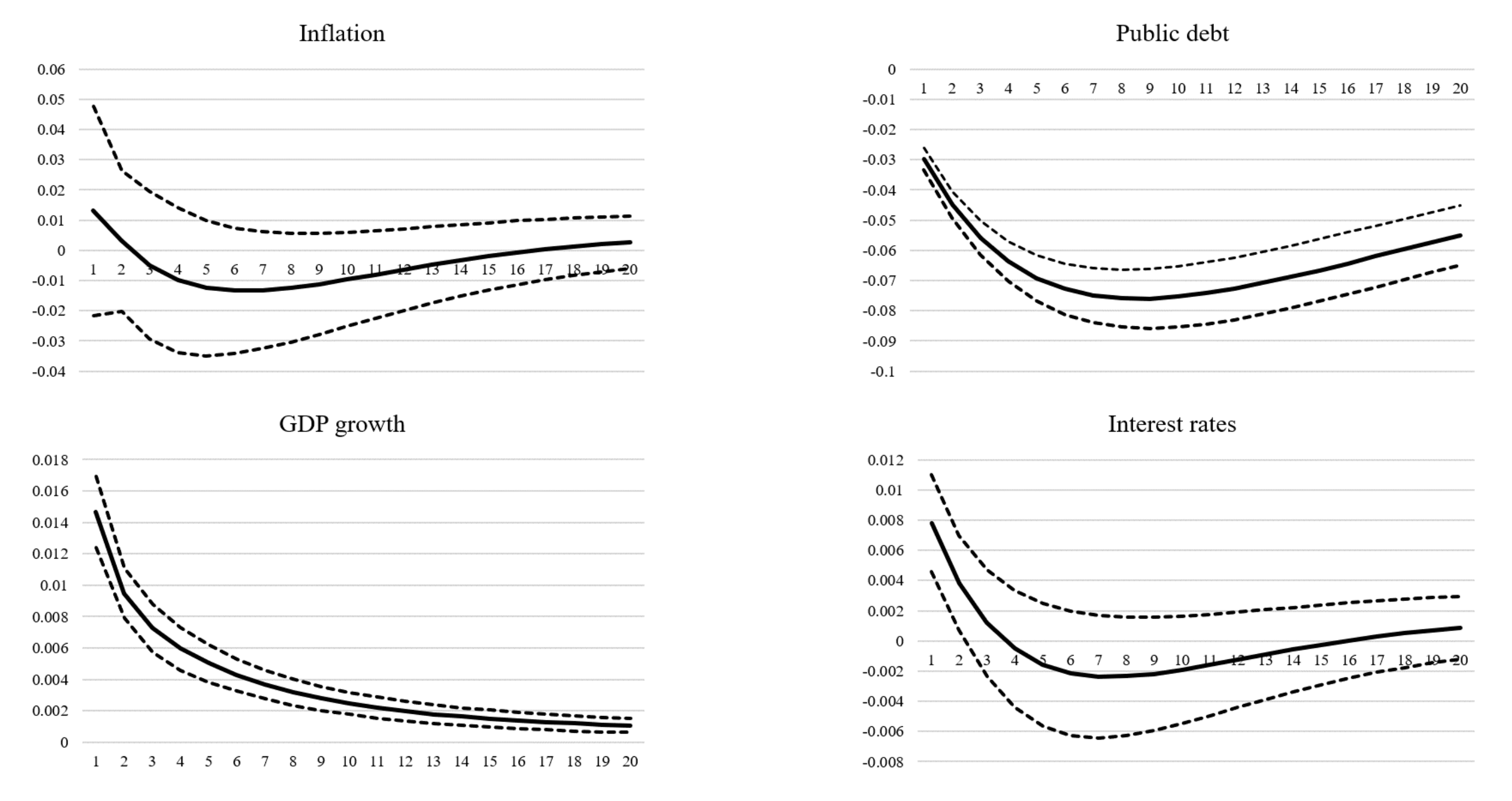
Figure 5.
Response to a positive shock to interest rates (with 95% confidence intervals).
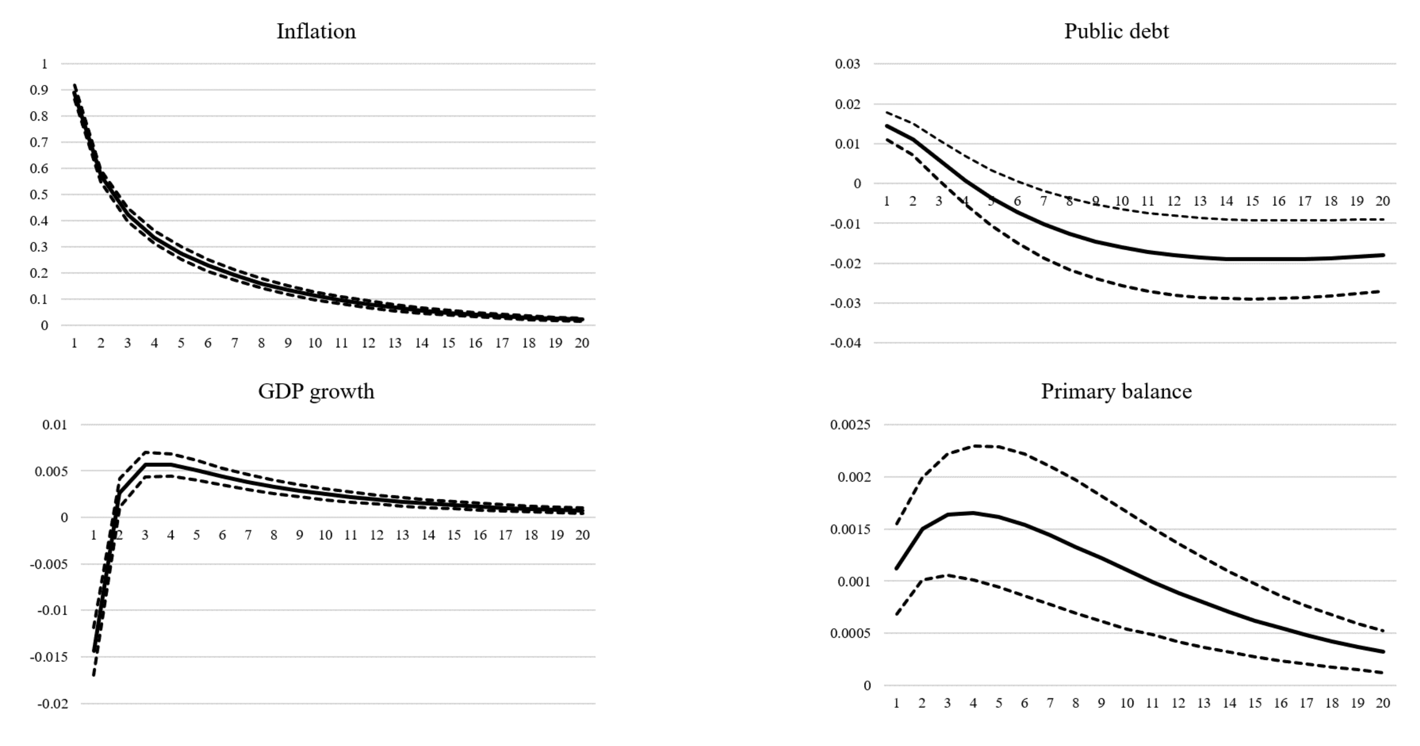
Figure 6.
Response to a negative shock to growth (with 95% confidence intervals).
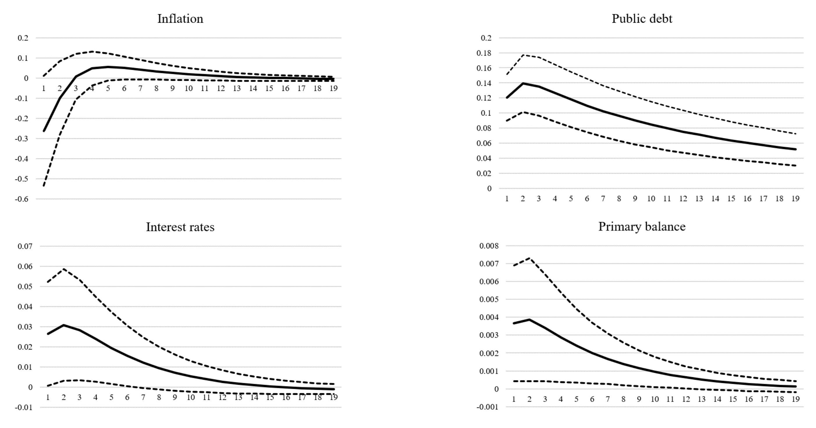
Figure 7.
Response of inflation to a positive shock to the primary balance by the monetary policy framework.
Figure 7.
Response of inflation to a positive shock to the primary balance by the monetary policy framework.
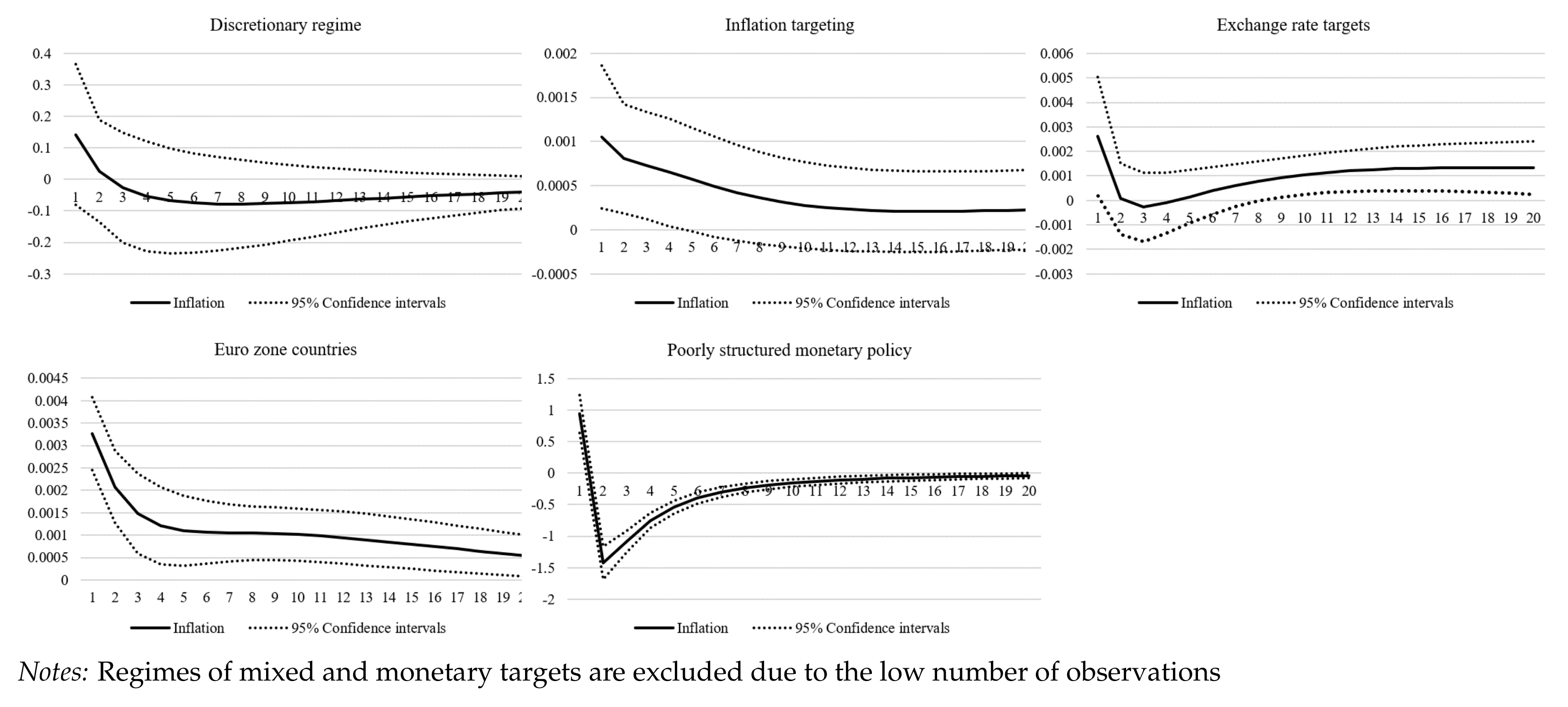
Figure 8.
Response of Inflation to a positive shock to interest rates by the monetary policy framework.
Figure 8.
Response of Inflation to a positive shock to interest rates by the monetary policy framework.
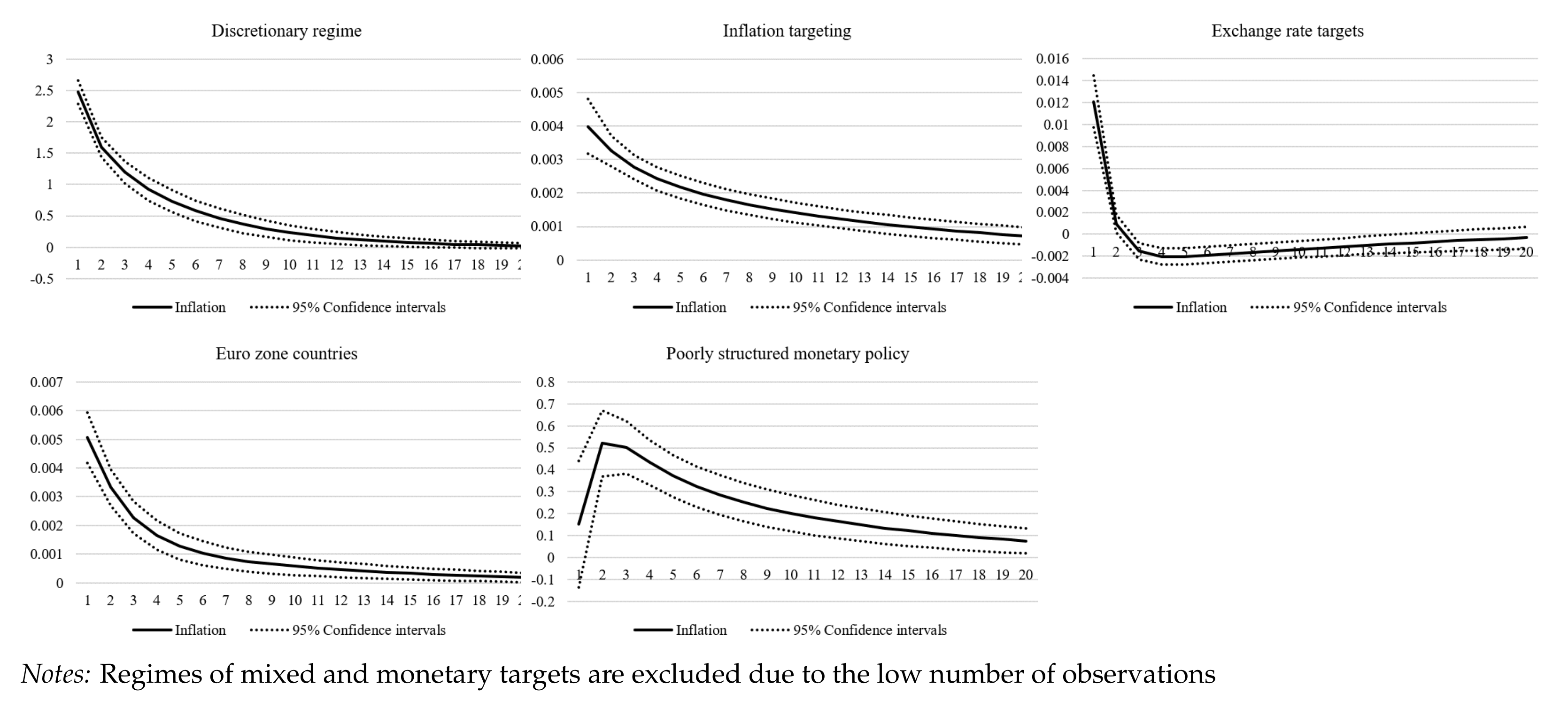
Figure 9.
Response of inflation to a negative shock to the primary balance by the monetary policy framework (with 95% confidence intervals).
Figure 9.
Response of inflation to a negative shock to the primary balance by the monetary policy framework (with 95% confidence intervals).
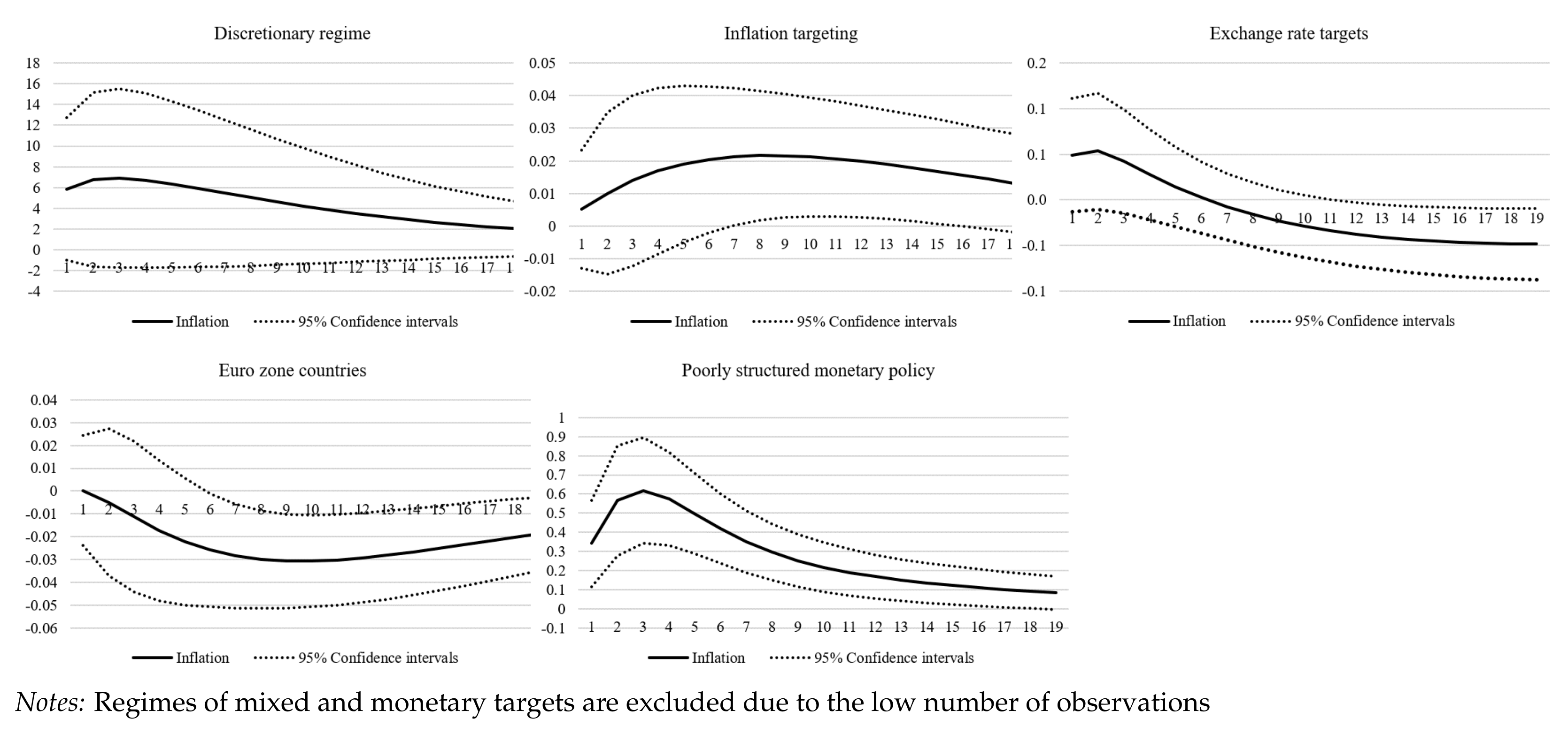
Figure 10.
Response of inflation to a one SD positive shock to the primary balance by the fiscal space group (with 95% confidence intervals).
Figure 10.
Response of inflation to a one SD positive shock to the primary balance by the fiscal space group (with 95% confidence intervals).
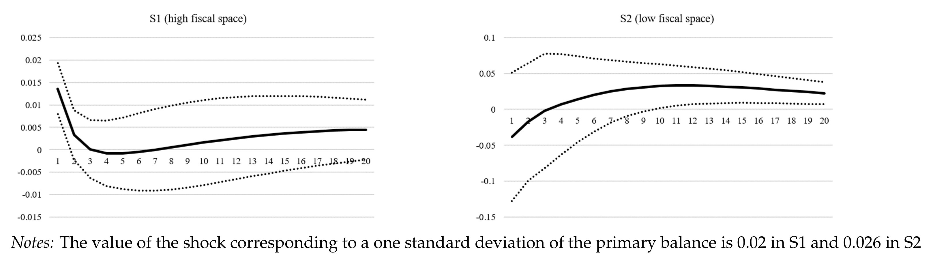
Figure 11.
Response of inflation to a one SD positive shock to interest rates by the fiscal space group (with 95% confidence intervals).
Figure 11.
Response of inflation to a one SD positive shock to interest rates by the fiscal space group (with 95% confidence intervals).
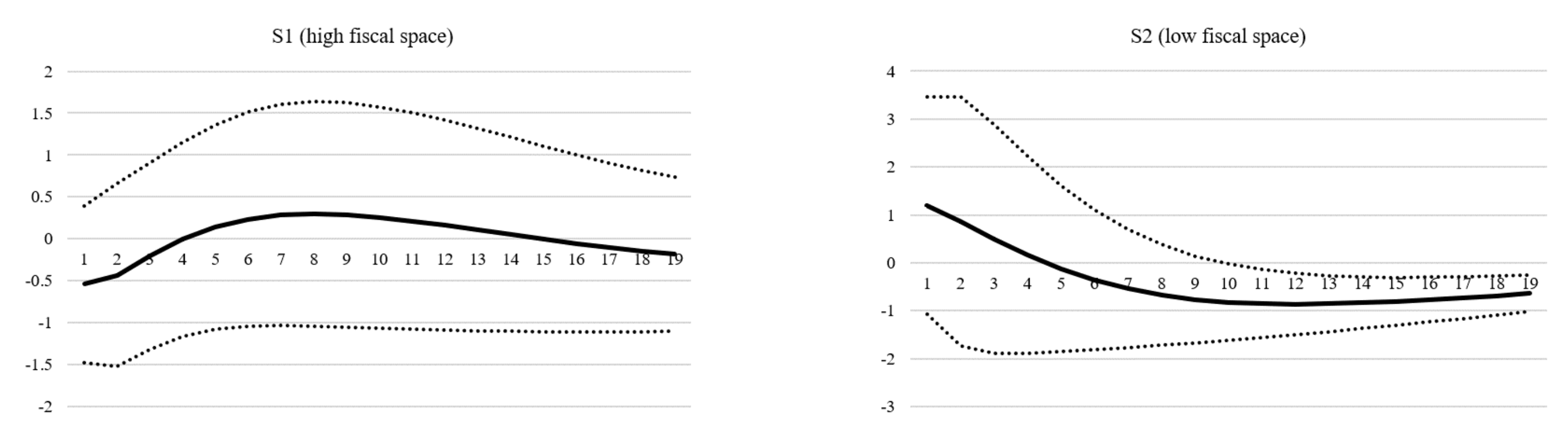
Figure 12.
Response of inflation to a negative shock to the primary balance by Fiscal space group (with 95% confidence intervals).
Figure 12.
Response of inflation to a negative shock to the primary balance by Fiscal space group (with 95% confidence intervals).

Figure 13.
Response of inflation to a shock to primary balances in low fiscal space countries (with 95% confidence intervals).
Figure 13.
Response of inflation to a shock to primary balances in low fiscal space countries (with 95% confidence intervals).
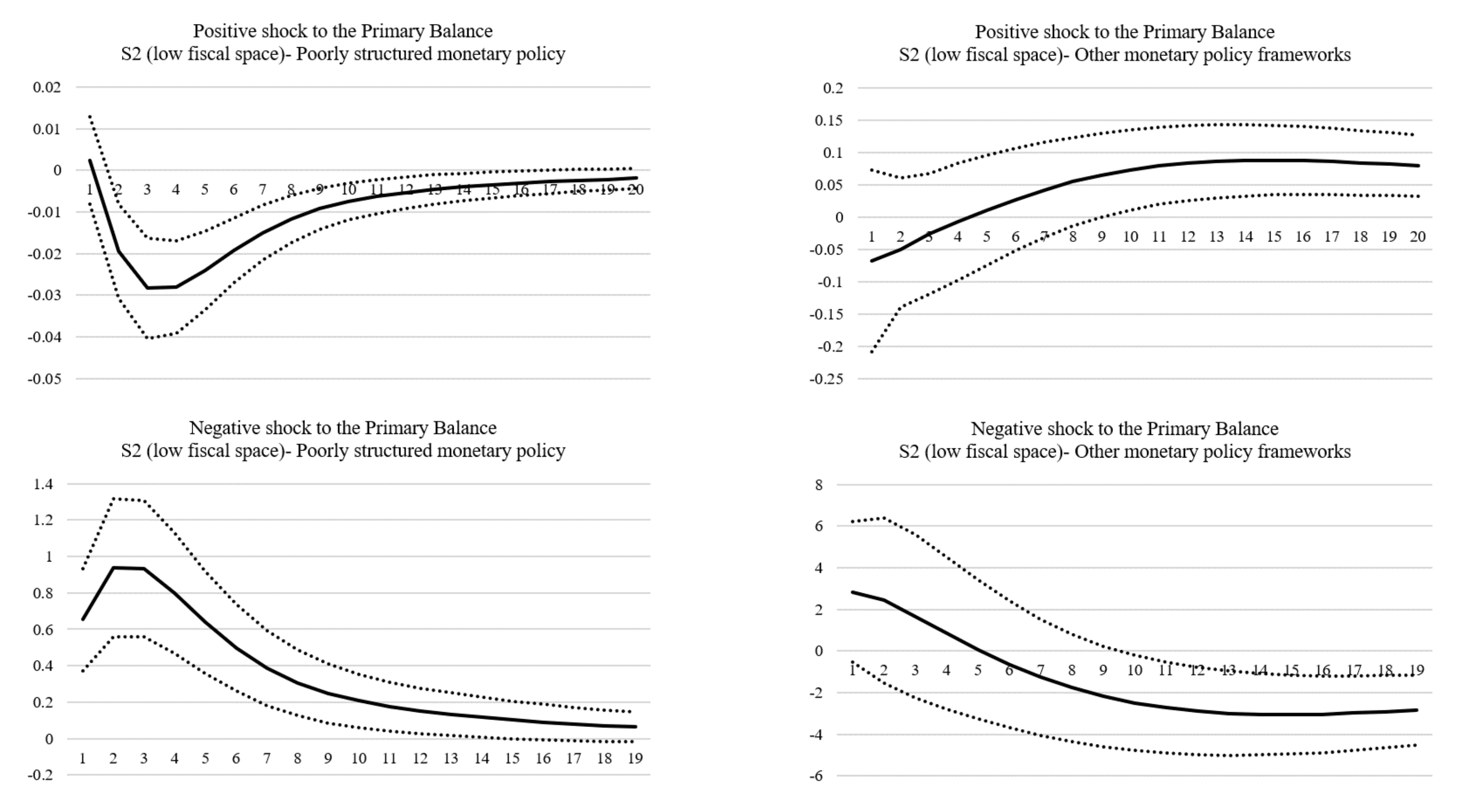
Table 2.
Correlation coefficients between the model’s main variables.
| i | |||||
| 100% | |||||
| −14% | 100% | ||||
| 2% | −1% | 100% | |||
| i | 6% | −2% | 66% | 100% | |
| 17% | −21% | 3% | 0% | 100% |
Notes: : primary surplus over GDP, : log of public debt over GDP, : inflation rate, i: short-term interest rate, : growth rate of GDP per capita.
Table 3.
Correlation coefficients of inflation with interest rates and the primary balance by monetary policy framework.
Table 3.
Correlation coefficients of inflation with interest rates and the primary balance by monetary policy framework.
| Correlation | Inflation and Interest Rates | Inflation and Primary Balance |
|---|---|---|
| Discretionary regimes | 88% | 23% |
| Inflation targeting (IT) | 40% | 8% |
| Exchange rate targets (ERTs) | 51% | 15% |
| Euro zone countries | 87% | 1% |
| Poorly structured monetary policy | 28% | −15% |
| Mixed targets | 85% | −30% |
| Monetary targets (MTs) | 75% | −16% |
Notes: classification of the sample by monetary policy framework is based on the database of Cobham [31]. The categories of “Mixed targets” and “Monetary targets” contain a small number of observations over the sample period.
Table 4.
Correlation coefficients of inflation with the fiscal variables and interest rates by fiscal space categories.
Table 4.
Correlation coefficients of inflation with the fiscal variables and interest rates by fiscal space categories.
| Correlation | S1 | S2 | Global |
|---|---|---|---|
| Inflation/primary balance | 5% | 2% | 2% |
| Inflation/public debt | −1% | −5% | −1% |
| Inflation/short-term interest rate | 90% | 59% | 66% |
Notes: S1: high fiscal space (50th upper percentile); S2: low fiscal space (50th lower percentile).
Table 5.
Panel VAR OLS estimation.
| Reduced-Form VAR | |||||
| i | |||||
| Lag 1 | 0.818 *** | −0.652 *** | 0.241 *** | −0.120 | −0.903 |
| (0.012) | (0.099) | (0.064) | (0.086) | (0.872) | |
| Lag 1 | 0.000 | 0.950 *** | 0.011 *** | −0.007 | −0.017 |
| (0.001) | (0.005) | (0.003) | (0.005) | (0.046) | |
| Lag 1 | −0.004 | −0.121 *** | 0.238 *** | −0.026 | 0.262 |
| (0.004) | (0.030) | (0.020) | (0.026) | (0.268) | |
| Lag 1 i | 0.003 | −0.04 ** | 0.035 *** | 0.879 *** | 1.905 *** |
| (0.002) | (0.017) | (0.011) | (0.014) | (0.147) | |
| Lag 1 | 0.000 | 0.003 | 0.000 | −0.010 *** | 0.313 *** |
| (0.000) | (0.003) | (0.002) | (0.002) | (0.022) | |
| Contemporaneous coefficients | |||||
| i | |||||
| 1 | 1.33 *** | −0.352 *** | −0.506 *** | 1.758 | |
| (0.157) | (0.098) | (0.139) | (1.184) | ||
| 0 | 1 | 0.229*** | −0.043 * | −0.148 | |
| (0.012) | (0.018) | (0.156) | |||
| 0 | 0 | 1 | 0.151 *** | −0.795 *** | |
| (0.028) | (0.239) | ||||
| i | 0 | 0 | 0 | 1 | −5.789 *** |
| (0.168) | |||||
| 0 | 0 | 0 | 0 | 1 | |
Notes: *** p < 0.001, ** p < 0.01, * p < 0.05. Standard errors in brackets : primary surplus over GDP, : log public debt/GDP, : growth rate, i: interest rate, : inflation rate. Contemporaneous coefficients obtained through Cholesky orthogonalization using the ordering of the variables that is displayed on the table.
Table 6.
Panel VAR GMM Estimation.
| i | |||||
| Lag 1 | 1.7114 | −0.8006 | 0.4023 | −0.4802 | −1.8017 |
| (2.0556) | (0.4349) | (0.3776) | (1.7175) | (1.2941) | |
| Lag 1 | −0.0277 | 0.9658 *** | −0.0108 | 0.0439 | 0.0446 |
| (0.0669) | (0.0272) | (0.0161) | (0.0664) | (0.1062) | |
| Lag 1 | −0.2952 | −0.0748 | 0.4232 * | 0.5708 | 0.5075 |
| (0.5773) | (0.1943) | (0.1873) | (0.7334) | (0.4981) | |
| Lag 1 i | 0.0054 | −0.0394 | 0.0232 | 0.7009 ** | 2.1820 * |
| (0.3989) | (0.0987) | (0.0873) | (0.2465) | (1.0212) | |
| Lag 1 | −0.0155 | 0.0052 | 0.0028 | 0.0197 | 0.3060 *** |
| (0.098) | (0.0169) | (0.0207) | (0.0444) | (0.0867) |
Notes: *** p < 0.001, ** p < 0.01, * p < 0.05. Standard errors in brackets : primary surplus over GDP, : log public debt/GDP, : growth rate, i: interest rate, : inflation rate. Forward orthogonal transformation is applied to the variables. Hansen test of overidentified restrictions: (1450) = 37.26, probability = 1.
Publisher’s Note: MDPI stays neutral with regard to jurisdictional claims in published maps and institutional affiliations. |
© 2021 by the authors. Licensee MDPI, Basel, Switzerland. This article is an open access article distributed under the terms and conditions of the Creative Commons Attribution (CC BY) license (https://creativecommons.org/licenses/by/4.0/).
Share and Cite
MDPI and ACS Style
Bazzaoui, L.; Nagayasu, J. Is Inflation Fiscally Determined? Sustainability 2021, 13, 11306. https://doi.org/10.3390/su132011306
AMA Style
Bazzaoui L, Nagayasu J. Is Inflation Fiscally Determined? Sustainability. 2021; 13(20):11306. https://doi.org/10.3390/su132011306
Chicago/Turabian StyleBazzaoui, Lamia, and Jun Nagayasu. 2021. "Is Inflation Fiscally Determined?" Sustainability 13, no. 20: 11306. https://doi.org/10.3390/su132011306
Note that from the first issue of 2016, this journal uses article numbers instead of page numbers. See further details here.