The Fallow Period Plays an Important Role in Annual CH₄ Emission in a Rice Paddy in Southern Brazil

Abstract

Paddy fields are significant anthropogenic sources of methane (CH₄) emissions. In southern Brazil, rice is grown in lowland flooded areas once a year, followed by a long fallow period. This study aimed to measure CH₄ fluxes in a rice paddy field in southern Brazil during the rice-growing season of 2015/2016 and the following fallow period. The fluxes were estimated using the eddy covariance (EC) technique and soil chamber (SC). Diurnal and seasonal variations of CH₄ fluxes and potential meteorological drivers were analyzed. The CH₄ fluxes showed distinct diurnal variations in each analyzed subperiod (vegetative, reproductive, pre-harvest, no rice, and land preparation), characterized by a single-peak diurnal pattern. The variables that most influenced methane emissions were air and surface temperatures. In the growing season, the rice vegetative stage was responsible for most of the measured emissions. The accumulated annual emission estimated was 44.88 g CH₄ m⁻² y⁻¹, being 64% (28.50 g CH₄ m⁻²) due to the rice-growing season and 36% (16.38 g CH₄ m⁻²) due to the fallow period. These results show the importance of including fallow periods in strategies to mitigate methane emissions in flood irrigated rice-growing areas.

1. Introduction

Methane (CH₄) is one of the main greenhouse gases (GHG) and has a heating potential 28 times higher than carbon dioxide (CO₂) [1]. Today, roughly 40% of CH₄ emissions are from natural sources, being the remainder caused by fossil fuels, the construction of hydroelectric dams, ruminant animals, landfills, and paddy fields [2,3,4,5,6].

Flooded rice fields are responsible for 11–26% of the total anthropogenic CH₄ emissions and emit around 30–40 Tg CH₄ per year, with Asia accounting for 90% of emissions [1]. Additionally, these rice are generally grown in lowland areas and are major sources of CH₄ emissions [7,8]. In Brazil, 11.2 million tons of rice were produced in 2020 in a 1.67 million ha area [9], representing approximately 2.0% of world production [10]. In the 2019/2020 rice season, Rio Grande do Sul State, southern state of Brazil, produced about 8 million tons of rice in a 0.94 million ha area [11], in which river lowlands were developed to increase rice production.

Due to the subtropical climate in southern Brazil, only one annual rice-growing season is possible, unlike most of Asia with two annual rice-growing seasons [12,13]. As a result, the rice paddies in southern Brazil have a long fallow period and no commercial cultivation, and most researchers have focused only on estimating CH₄ emissions for the rice-growing season [14,15,16,17,18]. Nevertheless, this is not a singular characteristic of southern Brazil, as the lack of scientific evidence on the fallow periods is also recurrent in other countries [19,20]. Moreover, CH₄ fluxes may be smaller in the fallow period than in the growing season because of low CH₄ emission rates due to aerobic processes [21]. However, as the lowlands are characterized by poorly drained soils under anaerobic conditions, the simultaneous production of CH₄ by methanogenic bacteria [7]. Methane produced by methanogenic bacteria is controlled by methanotrophic bacteria in the aerobic zone and CH₄ emission is the net outcome of both production and oxidation processes [22,23,24]. Therefore, CH₄ fluxes in the fallow period need to be quantified to understand what processes is controlling the flux, moreover making it possible to generate highly reliable annual estimates [25].

Surface CH₄ emissions are mainly estimated using soil chamber (SC) and eddy covariance (EC) measurements. The SC method is the most commonly used technique and able to determine small gas fluxes [26], although these measurements are punctual in time and space and may not capture the flux dynamics at different time scales. In addition, this method can disturb the integrity of the soil surface, interfering in the gas exchange dynamics between the emitting source and the atmosphere, leading to overestimated or underestimated values [27,28,29]. On the other hand, the EC method measures gas exchange between the ecosystem and atmosphere without interfering with its dynamics, enabling continuous long-term measurements and capturing different types of temporal variability [30,31]. In irrigated rice fields, CH₄ emissions have diverged between 20% and 90% depending on the comparison period, although in general, the SC method overestimates EC [32,33].

Furthermore, CH₄ flux measurements in flooded rice fields in southern Brazil have been carried out using the SC method, and no known studies have used the EC technique for such measurements. Therefore, this study aimed to fill this research gap by estimating CH₄ emissions in a paddy field using EC measurements throughout a growing season and a fallow period. In addition, we hypothesized that the fallow period could contribute significatively to the annual emissions of the paddy field. The objectives were to (1) quantify CH₄ emissions of a paddy field in southern Brazil; (2) describe the diurnal CH₄ flux patterns for the rice-growing season and fallow periods; (3) determine the meteorological factors that influence CH₄ emissions in different periods; (4) and compare EC and SC measurements in the same period.

2. Materials and Methods

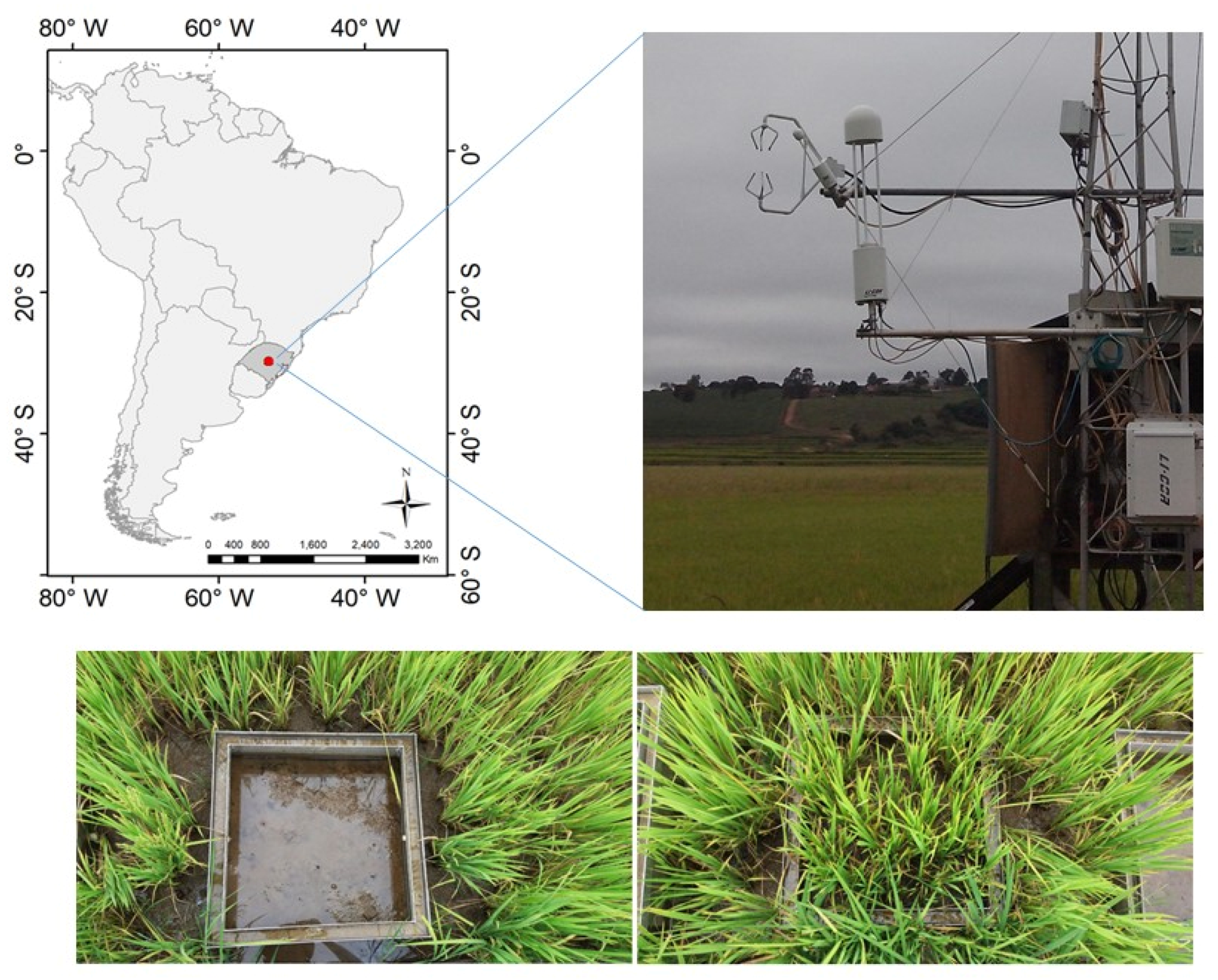
2.1. Site Description

The experimental site was located on a commercial rice farm (~1000 ha) in Cachoeira do Sul (30.27° S; 53.14° W; altitude: 40.5 m), Rio Grande do Sul State, Brazil (Figure 1). The climate is classified as humid subtropical (Cfa), according to Köppen [34]. The rice paddy was grown in a flooded system with dikes in 100 × 100 m plots. The average soil composition (5 cm depth) is 1.01% clay, 39.6% silt, and 59.34% sand. The soil organic carbon was 5.95 g Kg⁻¹ (0–5 cm layer). Further details about the experiment are described in Diaz et al. [35].

For this study, the 2015/2016 rice-growing season and following fallow period were evaluated. A late-cycle rice cultivar (Epagri 118) was planted on 5 November 2015, and harvested on 16 April 2016. Planting was carried out with pre-germinated seeds broadcast by airplane onto the flooded field with a standing water depth of 5 cm. The soil remained flooded with 5–10 cm of standing water during the growing season until one week before the harvest, and flooding was maintained by pumping water from the nearby river. The amount of N fertilizer applied was 68 kg N ha⁻¹, being in agreement with official technical recommendations for this region [36]. The average rice yield (Y) from the analyzed crop was 0.45 kg m⁻² (4.5 ton ha⁻¹). The rice phenological stages were estimated using the degree-day method [37]. This experimental site represents the rice paddy management system currently adopted by most farmers in southern Brazil.

2.2. Data Collection

A flux tower was installed in a dike of an irrigation channel in one of the rice fields (Figure 1), and data were collected from 21 November 2015 (16 days after planting, DAP) to 18 August 2016. Four static soil chambers (SC) were installed, side by side, ~10 m from the flux tower. Rice was allowed to grow in three chambers, while in the fourth chamber the soil was devoid of vegetation. The SC measurements started 76 DAP (20 January 2016) in the rice field (hereafter SC cultivated) and 90 DAP (5 February 2016) in the area without rice plants (hereafter SC uncultivated). The last SC measurements occurred on 14 April 2016.

Leaf area index (LAI) data were obtained from the MOD15A2 product of the MODIS (Moderate Resolution Imaging Spectroradiometer) with an 8-day temporal resolution and 1 km spatial resolution. Souza et al. [38] compared LAI (MOD15A2) data with experimental measurements at the same Cachoeira do Sul site and reported similar seasonal behavior in most of the rice-growing season.

2.2.1. Soil Chamber (SC)

Surface CH₄ fluxes were measured by the manually operated static closed chamber (soil chamber), according to Bayer et al. [15]. Each chamber consisted of an aluminum base (0.64 × 0.64 × 0.20 m) and an aluminum cover of the same size. The bases were inserted 5 cm into the soil. Each base had an open bottom and sealable channels on the sides to facilitate water flow. The channels on the sides were sealed during air sampling events. Additional 20–30 cm aluminum extensions were stacked on the bases as the plants grew taller. The chamber volume was considered in CH₄ emission measurements. Each chamber cover had a rubber septum sampling port, a stainless steel thermometer, and a battery-operated fan to circulate and homogenize air within the apparatus. Chamber closing and initial air sampling began at 9:00 a.m. local time. Air samples were taken at 0, 5, 10, and 20 min after closing the chamber [15]. Air samples were obtained by polypropylene syringes, transferred to evacuated 12-mL vials, and analyzed for CH₄ by gas chromatograph. The chromatograph (Shimadzu GC 2014 “Greenhouse”) was equipped with three packed columns at 70 °C, N₂ as carrier gas at a flow of 26 mL min⁻¹, an injector with 1 mL sample loop for direct injection at 250 °C, and a flame ionization detector (FID) at 250 °C for CH₄ detection. Air was sampled on a weekly basis during rice-growing season.

The CH₄ flux rates were calculated as follows [15]:

$$f=\frac{\Delta Q}{\Delta t}\frac{PV}{RT}\frac{M}{A}$$

(1)

where f is the CH₄ production rate (g m⁻² h⁻¹); ΔQ/Δt is the change in gas concentration (mol h⁻¹); P is the atmospheric pressure in the chamber (1 atm); V is the chamber volume (L); R is the ideal gas constant (0.0825 atm L mol⁻¹ K⁻¹); T is the chamber temperature (K); M is the gas molar mass (g mol⁻¹), and A is the chamber basal area (m²). The gas production rate was subsequently converted to μmol CH₄ m⁻² s⁻¹, with an average of the three rice chambers being calculated to obtain a single value representative of the rice field. The mean CH₄ flux from the air samples in each chamber was assumed to be equivalent to the mean daily flux [39]. Seasonal emissions were calculated by trapezoidal interpolation of the daily CH₄ fluxes during the evaluated period [15].

2.2.2. Eddy Covariance and Meteorological Measurements

The CH₄ concentrations were measured in the flux tower with an open-path gas analyzer using wavelength modulation spectroscopy (LI-7700, LI-COR Inc., Lincoln, NE, USA). Wind speed was measured with a three-dimensional sonic anemometer (CSAT3, Campbell Scientific Inc., Logan, UT, USA). Both sensors were installed 3 m above the ground. Data were recorded at 10 Hz via an analyzer interface unit (LI-7550, LI-COR Inc., Lincoln, NE, USA) and stored on a 16 GB hard drive.

Meteorological data were collected at 1 Hz using a data logger (CR1000, Campbell Scientific Inc., Logan, UT, USA). Air temperature (Tair) and relative humidity (RH) were measured using a thermohygrometer (CS215, Campbell Scientific Inc., Logan, UT, USA) installed 3 m above the ground. A rain gauge (TB4 Rain Gauge; Campbell Scientific Inc., Logan, UT, USA) 6 m above the ground measured precipitation (Prec). Photosynthetically active radiation (PAR) was measured at 4 m height using a quantum sensor (LI-190S, LI-COR Inc., Lincoln, NE, USA). Incident longwave (Ld) and emitted longwave (Lu) radiation were measured using a pyrgeometer (CGR3, Kipp & Zonen B.V., Delft, The Netherlands), and incident shortwave (Sd) and reflected shortwave (Su) radiation were measured using pyranometers (CMP3, Kipp & Zonen B.V., Delft, The Netherlands), which were all installed 5.6 m above the ground. Surface temperatures (Tskin) were measured using an infrared temperature sensor (SI-111, Apogee Instruments Inc., Logan, UT, USA). Soil temperatures (Tsoil) were measured at 5 cm depth using a thermometer (T-108, Campbell Scientific Inc., Logan, UT, USA), while soil heat flux (G) was measured at 15 cm depth using a heat flux plate (HFP01, Hukseflux Thermal Sensor Inc., Delft, The Netherlands). Soil water content (SWC) was measured using a reflectometer (CS616 water content reflectometer, Campbell Scientific Inc., Logan, UT, USA) at 30 cm depth. More details on the experimental site, data acquisition, and data processing are described in Diaz et al. [35] and Souza et al. [38].

2.3. Eddy Covariance Flux Data Processing

There were some technical problems until a useful dataset of CH₄ fluxes by EC was acquired (see Supplementary Material). The methane flux (CH₄ flux) was estimated using EC and consisted of calculating the covariance between turbulent fluctuations in the vertical wind speed and CH₄ concentration [30]. The CH₄ fluxes were measured at half-hour intervals using the EddyPro^® software, version 7 (Li-Cor, Lincoln, NE, USA). The raw data were filtered according to Vickers and Mahrt [40] and the peak counting and removal method proposed by Mauder et al. [41]. Turbulent fluctuations were also calculated in mean per block, with double rotation [42], correction of the density effect [43], flux mitigation due to instrument configuration [44], and high and low corrections of the filter according to the methods of Moncrieff et al. [45] and Moncrieff et al. [46], respectively.

EddyPro^® calculates three quality indicators for the CH₄ flux: 0 represents a good quality, 1 represents an intermediate quality, and 2 represents a low quality. Flux data with quality flags 1 and 2 were discarded. Moreover, CH₄ fluxes were discarded if the statistical quality of the raw time series failed (rigid flag test) in the following situations: spikes, amplitude resolution, dropouts, absolute limits, skewness and kurtosis, discontinuities, and time lag; in the case of failure in the rigid flags; when the relative signal strength indicator (RSSI) at the diagnostic output of the LI-7700 was below 10% [47,48,49]; in precipitation events and the following half-hour period [50]; and with values below −1 µmol CH₄ m⁻² s⁻¹ and above 1 µmol CH₄ m⁻² s⁻¹ that were established as physical limits for the experimental site. The limiting values of the friction velocity parameter (u*), which represent a situation of low turbulence, were estimated according to the method by Diaz et al. [35] for CO₂ flux in the same experimental site and period according to Reichstein et al. [51]. Values of CH₄ fluxes for u* threshold (u* < 0.11 m s⁻¹) were also discarded.

2.4. Gap-Filling and Uncertainty

During the study period, 5.5% missing half-hourly values for the meteorological and soil data were gap-filled using the REddyProc package (version 1.1.5) for RStudio software [51]. The precipitation data were not gap-filled and the whole day of these data were disregarded when they had more than 10% of failures.

Regarding the CH₄ fluxes measured by EC, 50.0% of the half-hour periods were lost due to equipment failure, and 23.5% were discarded for quality control. These gaps were gap-filled using an artificial neural network. According to Kim et al. [52], random forest (RF) performed well in filling CH₄ gaps across different sites, including rice paddies. In this way, we used the “randomForest” R package [53], which was implemented with 400 regression trees. In the exploratory analysis, were selected meteorological variables that show correlation index with CH₄ fluxes above 0.4 (results of Section 3.2.), including three fuzzy variables (day of the year and cosine and sine functions with a year-long wavelength) [52,54]. The data were randomly split into 80% as the RF algorithm training dataset and 20% as the validation dataset. The division, training, and validation procedure was repeated 50 times, totaling 50 RFs. The RF statistical validation parameters varied between 0.86 and 0.92 for r (Pearson correlation coefficient), 0.06 and 0.07 μmol m⁻² s⁻¹ for the RMSE (root mean square error), and between −3.9 and 3.5 for the PBias (percent Bias). The CH₄ gaps were filled by median prediction of 50 RFs.

Uncertainties in CH₄ fluxes can be caused by random errors associated with the gap filling approach. We followed the method described by Anderson et al. [55] and Knox et al. [56] to quantify the uncertainty in the cumulative fluxes applying a Monte Carlo simulation. In this work, a Monte Carlo simulation was used to randomly draw 1000 random errors for every original measurement binned by 0.05 µmol CH₄ m⁻² s⁻¹ of flux magnitude to quantify the random uncertainty of cumulative fluxes, followed by computing the variance of the cumulative sums. For the gap-filled values, the combined gap-filling and random uncertainty were calculated from the variance of the cumulative sums of the 50 RF predictions. The total uncertainty in the cumulative fluxes was then calculated by adding the cumulative gap-filling and random measurement uncertainties in quadrature, assuming that these sources of error were independent and normally distributed [57]. The uncertainty was calculated for the period with EC data in the study area (21 November 2015, to 18 August 2016).

2.5. Data Analysis

The study period was divided into five sub-periods according to the rice phenological stages and successive soil management:

—

Vegetative stage: from 21 November 2015, (16 DAP) in the vegetative stage (V4) to 9 January 2016, (62 DAP) in V13;

—

Reproductive stage: from 10 January 2016, (63 DAP) in the reproductive stage (R0) to 19 March 2016, (131 DAP) in R9, i.e., complete maturation stage;

—

Pre-harvest stage: from 20 March 2016, (132 DAP) to 19 April 2016, (162 DAP);

—

No rice stage: 19 April 2016, to 1 August 2016;

—

Land preparation stage: the period of land preparation is when the land is plowed, from 2 August 2016, to 18 August 2016.

The vegetative, reproductive, and pre-harvest stages were integrated to represent the rice-growing season, and the no rice and land preparation stages represented the fallow period.

Before gap-filling, the CH₄ fluxes obtained from the EC were correlated with the available atmospheric and soil variables, throughout r, in different sub-periods. For this analysis, the CH₄ fluxes not gap-filled were used because the gap-fill procedure uses meteorological factors as the independent variables in the fitting process, which may introduce false relationships between the CH₄ fluxes and other factors into the dataset [48].

The correlation coefficient r is calculated as:

$$r=\frac{1}{\left(n-1\right)}{\displaystyle \sum }_{i=1}^n\left(\frac{O_i-\overline{O}}{{\sigma }_O}\right)\left(\frac{M_i-\overline{M}}{{\sigma }_M}\right)$$

(2)

where $O_i$ represents the ith experimental CH₄ flux value, $M_i$ represents the ith modeled value for a total of n observations, $\overline{O}$ and $\overline{M}$ are the observed and modeled mean value, and ${\sigma }_O$ and ${\sigma }_M$ are the standard deviation of observed and modeled data [58]. r is a measure of the strength of the linear relationship between two variables. If there is a perfect linear relationship with a positive slope between the two variables, r = 1; if there is a perfect linear relationship with a negative slope between the two variables r = −1; if there is no linear relationship between the variables, r = 0. The correlations were considered weak if r < |0.4|, moderate if |0.4| ≤ r < |0.7|, and strong if r ≥ |0.7|. The correlation coefficient was also used to evaluate the ANN to estimate the CH₄ fluxes, as described in Section 2.4. Additionally, the RMSE and PBias statistical indices [58] were used in this analysis and are presented below:

$$\mathrm{RMSE}={\left(\frac{{{\displaystyle \sum }}_{i=1}^n{\left(M_i-O_i\right)}^2}{n}\right)}^{\frac{1}{2}}$$

(3)

$$\mathrm{PBias}=\frac{{{\displaystyle \sum }}_{i=1}^n\left(M_i-O_i\right)}{{{\displaystyle \sum }}_{i=1}^n\left(O_i\right)}\times 100$$

(4)

Analysis of the daily and seasonal variations of the CH₄ fluxes were carried out for both EC and SC methods. To complete one year of data, we extrapolated the results of the period measured in situ with EC, which we considered with similar soil cover and environmental conditions, using the mean value of each period. To compare with other studies in the literature, daily average conversions were performed using the following conversion factors between units: 1 μmol CH₄ m⁻² s⁻¹ = 1.382 g CH₄ m⁻² d⁻¹ = 1.037 gC m⁻² d⁻¹.

3. Results and Discussion

3.1. Atmospheric and Soil Conditions

Daily variations of the environmental variables are shown in Figure 2. Soil temperature at 5 cm depth (Tsoil) had the highest daily temperature values with similar behavior to air (Tair) and surface temperatures (Tskin), which presented very close daily averages (Figure 2a). The daily temperatures varied by more than 20 °C between the growing season (summer) and fallow periods (winter). The maximum daily Tair was verified during the summer (27.9 °C), and the minimum Tair was determined during the winter (4.8 °C). The soil heat flux (G) was positive in almost the entire growing season, which suggests that the surface layer warms the subsoil, while the subsoil warms the surface layer in the fallow period (G < 0).

The seasonality between the summer (growing season) and winter (fallow) seasons in this region is characterized by global solar radiation (Sd), with maximum values around 50% lower in the winter than in the summer (Figure 2b). Similar behavior was observed in the PAR since it is practically a fixed percentage of Sd [59] and Su, although the latter also depends on albedo that in general, is lower in fallow periods [60]. The Ld and Lu decreased, in absolute values, by around 25% in winter from the summer values due to lower air and soil temperatures. The negative values for radiations indicate their direction from the surface to the atmosphere.

Climatically, precipitation is well distributed throughout the year in the study region [35,38], varying from 83.9 mm (April) to 157.4 mm (August). On 22–23 December 2015, the daily accumulated precipitation amounted to 115 and 94.2 mm, respectively (Figure 2c). After that there were nearly 30 days of no recorded precipitation. The regular precipitation returned in February 2016. Unfortunately, there was a long period without precipitation data collection in the experimental site due to equipment failure (after 25 March 2016), which was identified as a negative value in Figure 2c. However, the flooding in the rice paddy does not depend on precipitation because it was maintained by pumping water from the nearby river. In general, RH is high because the rice paddies cover large areas within a catchment, creating a microclimate with high amounts of water available for evapotranspiration [61]. The lowest daily average of RH was 59% in the summer when little rainfall occurred. The highest vapor pressure deficit (VPD) values were in the rice-growing period and mainly due to the high air temperatures, exceeding values of 15 hPa [38]. The daily average soil water content (SWC) at 30 cm depth recorded a maximum value of 0.4 m³ m⁻³ and a minimum of 0.27 m³ m⁻³, being always above the soil field capacity, which is 0.21 m³ m⁻³ for this experimental site [35].

3.2. Correlation between the Meteorological Conditions and CH₄ Fluxes Not Gap-Filled

The factors influencing CH₄ emissions may contribute differently to the analyzed periods due to seasonal variations in atmospheric conditions and land use. In this study, we analyzed the correlations between the CH₄ fluxes obtained by the EC without gap-filling and atmospheric and soil variables at a half-hour basis for the entire period and different subperiods (Figure 3). The variables Tair, Tskin, and Lu presented moderate or high correlations in all subperiods. The negative correlation with Lu was obtained because negative values were used for this variable (Figure 1), i.e., the largest negative values represent higher longwave radiation emissions on the surface (the same analysis can be done for Su, but reflecting Sd). The correlations with Lu were very similar to Tskin, but with an inverted sign, which is expected since Lu depends directly on the surface temperature according to Stefan-Boltzmann’s law. A higher correlation between the CH₄ flux with Lu than with Tskin, despite slightly higher, must be related to the position of the sensor on the flux tower. The Lu sensor was installed 5.6 m above the ground and represents a larger and more homogeneous area than the Tskin sensor, which was installed 2.2 m above the ground and may represent either a more open area or with more plants. Except for the no rice subperiod, Tsoil and G also showed a moderate or high correlation in all subperiods. During land preparation, only Tsoil, Ld, and SWC had r below 0.6. Since the soil temperature is the variable as the main controller of methane fluxes [21,33,48,54,62,63,64], the low correlations found here regarding the no rice and land preparation subperiods may be a result of the intermittent flooding caused by precipitation. In the pre-harvest period (drained soil), the correlation of the VPD with CH₄ flux decreased.

In the rice-growing season, the vegetative stage presented the most variables (9 in total) with a correlation greater than |0.5|. In the pre-harvest, no variable showed a correlation greater than |0.5|, which may be related to the area drainage as it changed the soil moisture conditions faster. The smallest correlations were for Ld and SWC in all subperiods.

3.3. CH₄ Flux Gap-Filling

The RFs were implemented with a completely random division of training and validation data. The random division of training and validation of the dataset avoids biasing toward data periods with more flux coverage. The statistical indices between the CH_4(EC) and CH₄ obtained by the median of the 50 RFs predictions for the entire period and different subperiods are listed in

Table 1. Statistical indexes between CH₄ fluxes estimated by EC and median RFs predictions.

	Entire Period	Vegetative	Reproductive	Pre Harv.	No Rice	Land Prep
CH4(EC) data coverage (%)	26.5	47.3	40.4	21.3	8.2	30.5
RMSE (μmol m−2 s−1)	0.03	0.03	0.03	0.03	0.02	0.02
PBias (%)	0.40	0.30	0.60	−1.90	3.80	−0.20
r	0.98	0.99	0.97	0.97	0.94	0.98

. All statistical indices for the entire period showed better values than the validation of the 50 RFs. This means that the median of the CH₄ fluxes predicted by the RFs better represents the measured data than each RF individually. Satisfactory statistical indices were found for all the rice cultivation periods and land preparation. Despite the RMSE being low in the No rice and Pre-harvest periods, the PBias was higher in these periods, overestimating No rice and underestimating Pre-harvesting, which was likely caused by the smaller data coverage.

There is currently no consensus regarding CH₄ gap-filling methods due to limited comparative research [52]. Implementing a neural network method is complex, and its applicability depends on the favorable temporal representation of variables and data availability. Nevertheless, the ability of the neural network to model data with variable periodicity from the functional relationship between dependent and independent variables has increased its use for gap-filling (CH₄) flux time series [54,65,66,67]. Generally speaking, the network used herein (RF) is a good choice for gap-filling (CH₄) and has shown the best results compared to other networks, as reported by Kim et al. [52].

3.4. Seasonal and Diurnal CH₄ Fluxes

3.4.1. EC

The vegetative period had significant variation and a higher daily average of CH_4(EC) fluxes, with a daily average of approximately 0.18 g CH_4(EC) m⁻² d⁻¹ and a maximum of 0.44 g CH_4(EC) m⁻² d⁻¹ on 8 December 2015 (Figure 4). In this period, the main pathway of CH₄ transport between the soil and atmosphere occurs via aerenchyma in the root and stems of vascular plants [68,69]. Moreover, the daily average of CH_4(EC) fluxes significantly decreased during the period in which a large volume of precipitation was recorded (Figure 2), which is likely due to the lower Tsoil and VPD. Afterward, at the beginning of the reproductive stage with no precipitation and high soil temperature and VPD, the CH_4(EC) fluxes increased again, decreasing after the return of precipitation. This relationship is also confirmed by the high correlation between CH₄ and VPD, Tskin, and Tsoil (Figure 3) for this period (r = 0.72, 0.64, and 0.62, respectively). The LAI also increased quickly in this period, reaching 3.2 m² m⁻². The average value in the reproductive stage was slightly higher than in the vegetative period, with an average of 0.21 g CH_4(EC) m⁻² d⁻¹, although with lower values at the end of the period. As Weller et al. [62] reported, the reduced thermal amplitude within the canopy and soil layers due to increased LAI may be responsible for lower methane emissions as crops develop. In the pre-harvest period, the daily average was 0.16 g CH_4(EC) m⁻² d⁻¹, with values decreasing until the beginning of the no rice subperiod, which was the period with the smallest variations and CH_4(EC) fluxes, reaching values near zero (average value of 0.05 g CH_4(EC) m⁻² d⁻¹) due to aerobic conditions that stimulate methanotrophic bacteria development, which convert CH₄ into CO₂. During land preparation, fluxes increased once again (daily average of 0.09 g CH_4(EC) m⁻² d⁻¹) due to the supply of carbon derived from rice straw.

The daily cycle average of CH_4(EC) fluxes for each studied period is shown in Figure 5 with bootstrap confidence intervals (95%) in the mean. There is a diurnal pattern in CH_4(EC) fluxes in all periods. During the night, fluxes are almost constant and with little variation, and the highest values were found during the rice cultivation period. Furthermore, the CH_4(EC) fluxes increase at sunrise and peak around 3:00 p.m. (local time), decreasing significantly until sunset. This behavior is known as the single-peak diurnal pattern and is related to times with higher air and soil temperatures (data not shown). Similar results were also observed found by Hatala et al. [70], Knox et al. [54], and Ge et al. [48], analyzing daily cycle of CH_4(EC) over rice field in different place in the world.

The vegetative period presented the highest CH_4(EC) emission peaks and more significant variability of CH_4(EC) fluxes, with values of 0.34 μmol CH_4(EC) m⁻² s⁻¹. After the vegetative period, the peak emissions decreased, with values of 0.28 and 0.19 μmol CH_4(EC) m⁻² s⁻¹ for the reproductive and pre harvest periods, respectively. Considering the average for the entire rice-growing season (vegetative, reproductive, and pre-harvest), the maximum value was 0.28 μmol CH_4(EC) m⁻² s⁻¹. Alberto et al. [21] analyzed CH₄ emissions in a rice paddy in the Philippines and also reported a single-peak diurnal pattern during the growing season. The no rice period registered the lowest amplitudes with a maximum of 0.07 μmol CH_4(EC) m⁻² s⁻¹, while the land preparation period had, on average, a maximum value near the pre-harvest stage, 0.19 μmol CH_4(EC) m⁻² s⁻¹, although with more significant variability between the means. Nevertheless, the no rice and land preparation subperiods registered similar values during the night and showed the lowest values among all subperiods (~0.02 μmol CH_4(EC) m⁻² s⁻¹). For rice cultivation periods, these values were around 0.1 μmol CH_4(EC) m⁻² s⁻¹, with higher values in the pre-harvest subperiod.

3.4.2. SC

The CH₄ fluxes measured by the SC (hereafter CH_4(SC)) had similar seasonality to those obtained with EC, decreasing at the beginning of the reproductive stage and increasing until the middle of this period when CH_4(SC) fluxes decreased (Figure 4). At the beginning of the reproductive stage, the first two weekly samplings with the soil chambers showed lower CH_4(SC) flux values than those determined by EC (CH_4(EC)) (including a negative value, −0.07 ± 0.04 g CH_4(SC) m⁻² d⁻¹). From the third sampling on, the CH_4(SC) values were almost always higher than CH_4(EC), with maximum values of 0.61 ± 0.12 g CH_4(SC) m⁻² d⁻¹. Therefore, the measurements of soil chambers represented well the seasonal variability of CH_4(EC), increasing until half of the reproductive stage, shortly after decreasing. For the same period, uncultivated SC showed little variability in flux values with values around zero (maximum values of 0.04 g CH_4(SC) m⁻² d⁻¹ and minimum values of −0.019 g CH_4(SC) m⁻² d⁻¹). These values were similar to those obtained by EC during the fallow period, even without the water layer. Therefore, these results demonstrate the considerable emissions of CH₄ of the rice paddies, as also highlighted by Holzapfel-Pschorn and Seiler [71] and Schütz et al. [72].

In this study, the SC collections were carried out on clear days and under intense solar radiation (summer in the southern hemisphere), which may overestimate the CH₄ fluxes of the ecosystem. Moreover, the soil chambers are made of aluminum, which has high thermal conductivity, leading to quick temperature rises after closing and possibly altering gas fluxes due to the modified internal microenvironment, affecting microbiota activity and CH₄ transport processes [73]. The liquid CH₄ flux is controlled by bacteria that produce and consume CH₄, and three main processes carry out its transport in the rice paddy: transport through aerenchyma in roots and stems of vascular plants, ebullition as gas bubbles, and diffusion via the soil-floodwater interface [7]. The higher temperatures may also lead to different CH₄ concentrations between the soil surface and the top of the chamber [74,75]. Thus, three fans were installed inside each chamber to minimize these effects. Although the flux estimation using the chamber technique considers the temperature inside the chamber at the time of measurement (Equation (1)), the temperature has already changed the concentrations due to its effects on the transport processes. The effects of temperature may be minimized by insulating the chambers with thermal insulation material and protecting against direct solar radiation incidence, which is especially important in tropical and subtropical regions.

3.4.3. Annual Integrated Flux

During the entire EC analyzed period, from 21 November 2015, to 18 April 2016, the integrated CH₄ flux value was 36.05 ± 2.52 g CH_4(EC) m⁻² (±represents the total uncertainty of 7%). These CH₄ flux value results from simultaneous CH₄ production and consumption processes between the soil and the atmosphere, measured at the height of 3 m for 272 days. The daily accumulated CH₄ flux is presented in Figure 6. There are two periods with different average emission rates: one during the rice-growing season (vegetative, reproductive, and pre-harvest stages) and the other during the fallow period (no rice and land preparation). The change in the slope of the CH₄ accumulation curve occurred in April when the flood water was removed and the rice was harvested; hence, the CH_4(EC) emission rate decreased significantly. From 21 November 2015, to 18 April 2016 (growing season), an accumulated amount of 29.10 g CH_4(EC) m⁻² was recorded and equivalent to an emission rate of 0.19 g CH_4(EC) m⁻² d⁻¹, while from 19 April 2016, to 18 August 2016 (fallow period), 6.95 g CH_4(EC) m⁻² was recorded at a rate of 0.06 g CH_4(EC) m⁻² d⁻¹.

Schrier-Uijl et al. [32] proposed that the accumulated seasonal fluxes obtained by SC measurements can be calculated with models that consider the daily effects of temperatures on fluxes. However, in this study, we only used linear interpolation as it is the most widely used method and facilitates comparing results of other studies in the literature [16,76]. In the period that EC and SC measurements were performed simultaneously (5 February 2016, to 14 April 2016, totaling 70 days), the accumulated EC was 12.86 g CH_4(EC) m⁻², while the SC registered 22.5 g CH_4(SC) m⁻² for the cultivated plot and 1.1 g CH_4(SC) m⁻² for the uncultivated plot. Therefore, a SC for the cultivated plot measured a CH₄ emission that accumulated 74% higher than the EC in the same period. Studies have shown that fluxes measured with the SC method are greater in flooded areas (e.g., irrigated rice) than those with the EC method, with variations between 20 and 90% [76,77,78].

Possible reasons for the significant differences between SC and EC measurements could be the non-homogeneous characteristics of the surface in the field and different spatial and temporal scales of the collections. Chamber measurements capture emissions from small areas, which may not represent natural spatial variations in soil and plant growth because of possible irregular fertilizer spread or localized variations in water level [79]. In addition, weekly measurements are taken with the chambers, while half-hourly measurements are performed with the EC, capturing the diurnal variations in fluxes due to daily variations in climate and plant growth. Nonetheless, the EC data can also present gaps due to lack of power or after proper filtering of the data due to low turbulence, control quality, or the small CH₄ sensor (as described in Section 2.3). Thus, both methods need gap-filling to generate full periods of data. In general, the weekly data from the cameras are linearly interpolated and may present overestimation, as collections usually occur on days with clear skies, and climatic variations are not taken into account.

Using SC to estimate CH₄ fluxes in irrigated rice fields with and without rice plants (cultivated and uncultivated), it is estimated that rice plants contribute about 95% to CH₄ emissions from the soil to the atmosphere. This occurs due to the transport of gases by diffuse exchange and mainly by internal convective fluxes [21,64]. The internal convective CH₄ fluxes result from the pressure gradient in different parts of the plant [21]. Other authors have also reported the contribution of plants to CH₄ emission from the soil into the atmosphere, including Holzapfel-Pschorn and Seiler [71] and Schütz et al. [72], who estimated the contribution of rice plants for CH₄ emissions as 80 and 90%, respectively.

Unfortunately, the EC system did not have a full year of CH₄ flux measurements, which may characterize a limitation for this study. However, according to our results and similar studies with irrigated rice, CH₄ fluxes are high during the vegetative period (beginning of the vegetative phase until the end of pre-harvest period) and reduced during the fallow period until planting [20,21,33,76]. Therefore, to complete one year of data, we extrapolated the results of the period measured in situ, which we considered had similar soil cover and environmental conditions for days without measurements. For the days at the beginning of the growing season (between 5–20 November 2015), the average daily rate of CH₄ emission of the growing season (0.19 g CH_4(EC) m⁻² d⁻¹) was used. From 19 August 2016, to 4 November 2016, the average daily CH₄ emission rate for no rice and land preparation (0.06 g CH_4(EC) m⁻² d⁻¹) was used, thus completing 365 days. In general, two or three weeks after land preparation, the field is kept fallow until the next rice-growing season. Therefore, by extrapolating the results for one year, we reached the total annual accumulated value of 44.88 g CH_4(EC) m⁻² y⁻¹, with the rice-growing season being responsible for 28.50 g CH_4(EC) m⁻² and the fallow period for 16.38 g CH_4(EC) m⁻², i.e., the rice-growing season accounts for 64% of the annual CH₄ emission, while the fallow is responsible for 36%. Hence, the CH₄ emissions during the fallow period represent 57% of the emissions in the rice-growing season. The accumulated value of CH_4(EC) fluxes in the growing season may likely be lightly overestimated because we do not have CH₄ flux measurements in the first days after flooding, which is when emissions are lower [33]. In addition, emissions during the fallow period may have been overestimated, as the gap-filling method presented positive PBias in this period (Table 1). Although the number of gaps in this period increased, the lower diurnal variability in CH₄ fluxes may improve RF representation.

In a rice paddy in northern Italy and with similar management practices, Meijide et al. [76] obtained annual accumulated values of 37.42 and 21.03 g CH_4(EC) m⁻² for 2009 and 2010, respectively, i.e., approximately 17 and 53% lower than the values reported herein. These authors attributed the differences found in the two years to climatic conditions and mainly the water level in the field. These differences demonstrate the importance of long-term studies to understand interannual variability.

Several studies were carried out in southern Brazil to estimate CH₄ emissions using SC in different types of soil and water management systems. Bayer et al. [16] obtained a growing season accumulated average of 367 kg CH_4(SC) ha⁻¹ (36.7 g CH_4(SC) m⁻²) with a variation of 100 kg CH_4(SC) ha⁻¹ to 600 kg CH_4(SC) ha⁻¹ during seven harvests (2004–2013). Therefore, the average value was 22% higher than the obtained here (28.50 g CH_4(EC) m⁻²). Evaluating different rice management levels, including seed and fertilizer rates, irrigation, and pesticide use, Zschornack et al. [20] recorded the average accumulated CH₄ of the rice season (growing season) ranging from 250.9 kg CH_4(SC) ha⁻¹ (25.09 g CH_4(SC) m⁻²) to 671.5 kg CH_4(SC) ha⁻¹ (67.15 g CH_4(SC) m⁻²), and the fallow ranging from 0.9 kg CH_4(SC) ha⁻¹ (0.09 g CH_4(SC) m⁻²) to 58.1 kg CH_4(SC) ha⁻¹ (5.81 g CH_4(SC) m⁻²). In these cases, the fallow contributes between 0.1 to 19% of the annual CH₄ emissions, which is lower than the percentage evidence here using EC (35%).

A critical comparison to be done is with the CH₄ emission factor for rice fields, as proposed by IPCC [80]. The IPCC [80] emission factor for the growing season is estimated as 0.13 g CH₄ m⁻² d⁻¹, being almost 30% lower than the value reported herein (0.19 g CH_4(EC) m⁻² d⁻¹), representing a significant underestimation of CH₄ emission in rice paddy fields in southern Brazil.

CH₄ has a global warming potential (GWP) 28 times greater than CO₂, while N₂O has a contribution 265 times greater than the CO₂ (both for a 100-year time horizon not considering the climate-carbon feedbacks [1]). Nonetheless, N₂O had an almost insignificant contribution in the rice paddies [16,76], and this is because the N₂O is mostly converted into N₂ via denitrification under flooded soil conditions [81]. Hence, by converting the CH₄ into CO_2-eq, the rice-growing season was responsible for 798 g CO_2-eq m⁻² and the fallow period for 458 g CO_2-eq m⁻². In a previous study by our research group, Diaz et al. [35] estimated the CO₂ net exchange ecosystem (NEE) for five years in the same experimental area (20 October 2010 to 16 April 2016) and reported that the NEE = −1334 g CO₂ m⁻² for the same rice paddy growing season (2015/2016) and NEE = 981 g CO₂ m⁻² for the fallow period in five-year average (2011–2015). By adding the contributions of CO₂ and CH₄ in the partial GWP (GWPp), the growing season GWPp represents an absorber of −536 g CO_2-eq m⁻², while the GWPp represents an emitter of 1439 g CO_2-eq m⁻² in the fallow period, totaling at an annual emission of 903 g CO_2-eq m⁻². Therefore, CH₄ was dominantly responsible for the GWPp, as also reported by Meijide et al. [76]. The CH₄ emitter in the fallow accounted for almost 50% of the annual GWPp. Furthermore, the fallow emitted almost threefold the GWPp that was absorbed by the growing season. As 450 g of rice was produced in the growing season, we can consider that for each gram of rice produced, 2.0 g CO_2-eq was annually emitted per area, making the irrigated rice cultivation area a strong emitter of greenhouse gases.

4. Conclusions

This study presents the first CH₄ estimates using eddy covariance in a paddy field in southern Brazil, covering a growing season and a fallow period. The diurnal and seasonal variations of CH₄ fluxes were analyzed. The seasonal integrations showed that the rice-growing season emitted 28.50 g CH₄ m⁻² and the fallow period emitted 16.38 g CH₄ m⁻², i.e., the fallow emitted 35% of annual CH₄ flux. Although lower than the growing season, the emission in fallow is significant to the annual estimation. The diurnal cycle was characterized by a single-peak diurnal pattern in different phenological stages and the fallow period. The most significant daily CH₄ flux variation and highest values occurred during the vegetative stage. Air and surface temperatures were the variables that most influenced those dynamics.

Measuring CH₄ fluxes using EC and SC in the cultivated plot was compared for the reproductive and pre-harvest stages, resulting in SC overestimating EC by 74%. Nevertheless, a comparison of integrated CH₄ fluxes from EC in the growing season with other studies using SC in southern Brazil demonstrated similar findings. In uncultivated plots, the CH₄ flux from SC was similar to those obtained using EC during the fallow period. Moreover, the SC results shows that rice plants contribute about 95% to CH₄ emissions from the soil to the atmosphere, highlighting the importance of rice cultivation in the CH₄ emission rate.

Using estimates based on EC to obtain annual integrations of GWPp, our results show that the paddy field is an annual sink of 903 g CO_2-eq m⁻². The fallow emitted almost threefold the GWPp that was absorbed by the rice-growing season. This study adds further support to the evidence that CH₄ emissions from areas used for flood irrigated rice cultivation significantly influence annual carbon balances and GWP. Therefore, it is fundamental to stimulate technological practices that reduce CH₄ emissions in the rice-growing season of different processes and during the fallow period.

As a complementary part of this work, our results can be used in the verification and calibration of the Brazilian Global Atmospheric Model—BAM [82], the atmospheric component of the Brazilian Earth System Model (BESM), since no studies including CH₄ flux emissions over paddy field in southern Brazil have been carried out with this model.

References

1. IPCC. Intergovernamental Panel on Climate Change: Working Group I Contribution to the Fifth Assessment Report of the Intergovernamental Panel on Climate Change; Stocker, T., Qin, D., Plattner, G., Tignor, M., Allen, S., Boschung, J., Nauels, A., Xia, Y., Vincent Bex, P.M., Eds.; Cambridge University Press: New York, NY, USA, 2013; ISBN 9781107661820. [Google Scholar]
2. Wuebbles, D.J.; Hayhoe, K. Atmospheric methane and global change. Earth-Sci. Rev. 2002, 57, 177–210. [Google Scholar] [CrossRef]
3. Lelieveld, J. Climate change: A nasty surprise in the greenhouse. Nature 2006, 443, 405–406. [Google Scholar] [CrossRef]
4. Baldocchi, D.; Detto, M.; Sonnentag, O.; Verfaillie, J.; Teh, Y.A.; Silver, W.; Kelly, N.M. The challenges of measuring methane fluxes and concentrations over a peatland pasture. Agric. For. Meteorol. 2012, 153, 177–187. [Google Scholar] [CrossRef]
5. Ul-Haq, Z.; Tariq, S.; Ali, M. Atmospheric variability of methane over Pakistan, Afghanistan and adjoining areas using retrievals from SCIAMACHY/ENVISAT. J. Atmos. Solar-Terr. Phys. 2015, 135, 161–173. [Google Scholar] [CrossRef]
6. Savi, F.; Di Bene, C.; Canfora, L.; Mondini, C.; Fares, S. Environmental and biological controls on CH4 exchange over an evergreen Mediterranean forest. Agric. For. Meteorol. 2016, 226–227, 67–79. [Google Scholar] [CrossRef]
7. Conrad, R. Microbial Ecology of Methanogens and Methanotrophs. Adv. Agron. 2007, 96, 1–63. [Google Scholar]
8. Malyan, S.K.; Bhatia, A.; Kumar, A.; Gupta, D.K.; Singh, R.; Kumar, S.S.; Tomer, R.; Kumar, O.; Jain, N. Methane production, oxidation and mitigation: A mechanistic understanding and comprehensive evaluation of influencing factors. Sci. Total Environ. 2016, 572, 874–896. [Google Scholar] [CrossRef] [PubMed]
9. Conab Companhia Nacional de Abastecimento. Available online: https://www.conab.gov.br/ (accessed on 10 April 2021).
10. USDA (United States Department of Agriculture). Foreign Agricultural Service. Available online: https://apps.fas.usda.gov/psdonline/circulars/production.pdf (accessed on 9 September 2021).
11. IRGA Instituto Rio Grandense do Arroz. Available online: https://irga.rs.gov.br/inicial (accessed on 10 April 2021).
12. Alberto, M.C.R.; Wassmann, R.; Hirano, T.; Miyata, A.; Hatano, R.; Kumar, A.; Padre, A.; Amante, M. Comparisons of energy balance and evapotranspiration between flooded and aerobic rice fields in the Philippines. Agric. Water Manag. 2011, 98, 1417–1430. [Google Scholar] [CrossRef]
13. Hossen, M.S.; Mano, M.; Miyata, A.; Baten, M.A.; Hiyama, T. Surface energy partitioning and evapotranspiration over a double-cropping paddy field in Bangladesh. Hydrol. Process. 2012, 26, 1311–1320. [Google Scholar] [CrossRef]
14. da Silva, L.S.; Griebeler, G.; Moterle, D.F.; Bayer, C.; Zschornack, T.; Pocojeski, E. Dinâmica da emissão de metano em solos sob cultivo de arroz irrigado no sul do Brasil. Rev. Bras. Cienc. Solo 2011, 35, 473–481. [Google Scholar] [CrossRef] [Green Version]
15. Bayer, C.; Costa, F.D.S.; Pedroso, G.M.; Zschornack, T.; Camargo, E.S.; de Lima, M.A.; Frigheto, R.T.S.; Gomes, J.; Marcolin, E.; Macedo, V.R.M. Yield-scaled greenhouse gas emissions from flood irrigated rice under long-term conventional tillage and no-till systems in a Humid Subtropical climate. Field Crops Res. 2014, 162, 60–69. [Google Scholar] [CrossRef]
16. Bayer, C.; Zschornack, T.; Pedroso, G.M.; da Rosa, C.M.; Camargo, E.S.; Boeni, M.; Marcolin, E.; dos Reis, C.E.S.; dos Santos, D.C. A seven-year study on the effects of fall soil tillage on yield-scaled greenhouse gas emission from flood irrigated rice in a humid subtropical climate. Soil Tillage Res. 2015, 145, 118–125. [Google Scholar] [CrossRef]
17. Camargo, E.S.; Pedroso, G.M.; Minamikawa, K.; Shiratori, Y.; Bayer, C. Intercontinental comparison of greenhouse gas emissions from irrigated rice fields under feasible water management practices: Brazil and Japan. Soil Sci. Plant Nutr. 2018, 64, 59–67. [Google Scholar] [CrossRef] [Green Version]
18. Chirinda, N.; Arenas, L.; Katto, M.; Loaiza, S.; Correa, F.; Isthitani, M.; Loboguerrero, A.; Martínez-Barón, D.; Graterol, E.; Jaramillo, S.; et al. Sustainable and Low Greenhouse Gas Emitting Rice Production in Latin America and the Caribbean: A Review on the Transition from Ideality to Reality. Sustainability 2018, 10, 671. [Google Scholar] [CrossRef] [Green Version]
19. Reba, M.L.; Fong, B.N.; Rijal, I. Fallow season CO2 and CH4 fluxes from US mid-south rice-waterfowl habitats. Agric. For. Meteorol. 2019, 279, 107709. [Google Scholar] [CrossRef]
20. Zschornack, T.; da Rosa, C.M.; dos Reis, C.E.S.; Pedroso, G.M.; Camargo, E.S.; Dossantos, D.C.; Boeni, M.; Bayer, C. Soil CH4 and N2O emissions from rice paddy fields in southern Brazil as affected by crop management levels: A three-year field study. Rev. Bras. Cienc. Solo 2018, 42. [Google Scholar] [CrossRef] [Green Version]
21. Alberto, M.C.R.; Wassmann, R.; Buresh, R.J.; Quilty, J.R.; Correa, T.Q.; Sandro, J.M.; Centeno, C.A.R. Measuring methane flux from irrigated rice fields by eddy covariance method using open-path gas analyzer. Field Crops Res. 2014, 160, 12–21. [Google Scholar] [CrossRef]
22. Malyan, S.K.; Bhatia, A.; Tomer, R.; Harit, R.C.; Jain, N.; Bhowmik, A.; Kaushik, R. Mitigation of yield-scaled greenhouse gas emissions from irrigated rice through Azolla, Blue-green algae, and plant growth–promoting bacteria. Environ. Sci. Pollut. Res. 2021, 28, 51425–51439. [Google Scholar] [CrossRef] [PubMed]
23. Malyan, S.K.; Kumar, S.S.; Fagodiya, R.K.; Ghosh, P.; Kumar, A.; Singh, R.; Singh, L. Biochar for environmental sustainability in the energy-water-agroecosystem nexus. Renew. Sustain. Energy Rev. 2021, 149, 111379. [Google Scholar] [CrossRef]
24. Malyan, S.K.; Bhatia, A.; Kumar, S.S.; Fagodiya, R.K.; Pugazhendhi, A.; Duc, P.A. Mitigation of greenhouse gas intensity by supplementing with Azolla and moderating the dose of nitrogen fertilizer. Biocatal. Agric. Biotechnol. 2019, 20, 101266. [Google Scholar] [CrossRef]
25. Morin, T.H. Advances in the Eddy Covariance Approach to CH 4 Monitoring Over Two and a Half Decades. J. Geophys. Res. Biogeosci. 2019, 124, 453–460. [Google Scholar] [CrossRef] [Green Version]
26. Denmead, O.T. Approaches to measuring fluxes of methane and nitrous oxide between landscapes and the atmosphere. Plant Soil 2008, 309, 5–24. [Google Scholar] [CrossRef]
27. Hendriks, D.M.D.; van Huissteden, J.; Dolman, A.J. Multi-technique assessment of spatial and temporal variability of methane fluxes in a peat meadow. Agric. For. Meteorol. 2010, 150, 757–774. [Google Scholar] [CrossRef]
28. McDermitt, D.; Burba, G.; Xu, L.; Anderson, T.; Komissarov, A.; Riensche, B.; Schedlbauer, J.; Starr, G.; Zona, D.; Oechel, W.; et al. A new low-power, open-path instrument for measuring methane flux by eddy covariance. Appl. Phys. B Lasers Opt. 2011, 102, 391–405. [Google Scholar] [CrossRef]
29. Peltola, O.; Hensen, A.; Belelli Marchesini, L.; Helfter, C.; Bosveld, F.C.; van den Bulk, W.C.M.; Haapanala, S.; van Huissteden, J.; Laurila, T.; Lindroth, A.; et al. Studying the spatial variability of methane flux with five eddy covariance towers of varying height. Agric. For. Meteorol. 2015, 214–215, 456–472. [Google Scholar] [CrossRef]
30. Baldocchi, D.D.; Hicks, B.B.; Meyers, T.P. Measuring biosphere-atmosphere exchanges of biologically related gases with micrometeorological methods. Ecology 1988, 69, 1331–1340. [Google Scholar] [CrossRef]
31. Baldocchi, D.D. How eddy covariance flux measurements have contributed to our understanding of Global Change Biology. Glob. Chang. Biol. 2020, 26, 242–260. [Google Scholar] [CrossRef]
32. Schrier-Uijl, A.P.; Kroon, P.S.; Hensen, A.; Leffelaar, P.A.; Berendse, F.; Veenendaal, E.M. Comparison of chamber and eddy covariance-based CO2 and CH4 emission estimates in a heterogeneous grass ecosystem on peat. Agric. For. Meteorol. 2010, 150, 825–831. [Google Scholar] [CrossRef] [Green Version]
33. Meijide, A.; Manca, G.; Goded, I.; Magliulo, V.; Di Tommasi, P.; Seufert, G.; Cescatti, A. Seasonal trends and environmental controls of methane emissions in a rice paddy field in Northern Italy. Biogeosciences 2011, 8, 3809–3821. [Google Scholar] [CrossRef] [Green Version]
34. Peel, M.C.; Finlayson, B.L.; McMahon, T.A. Updated world map of the Köppen-Geiger climate classification. Hydrol. Earth Syst. Sci. 2007, 11, 1633–1644. [Google Scholar] [CrossRef] [Green Version]
35. Diaz, M.B.; Roberti, D.R.; Carneiro, J.V.; Souza, V.D.A.; de Moraes, O.L.L. Dynamics of the superficial fluxes over a flooded rice paddy in southern Brazil. Agric. For. Meteorol. 2019, 276–277, 107650. [Google Scholar] [CrossRef]
36. EMBRAPA. Adubação e Calagem para o Arroz Irrigado no Rio Grande do Sul. Available online: https://www.infoteca.cnptia.embrapa.br/infoteca/bitstream/doc/745950/1/Circular62.pdf (accessed on 4 October 2021).
37. Steinmetz, S.; Cuadra, S.V.; Pereira, C.B.; Santos, E.L.; Almeida, I.R. GD Arroz: Programa Baseado em Graus-Dia como Suporte ao Planejamento e à Tomada de Decisão no Manejo do Arroz Irrigado; Embrapa Clima Temperado, Circular Técnica, 162; Embrapa Clima Temperado: Pelotas, Brazil, 2015; 8p. (In Portuguese) [Google Scholar]
38. Souza, V.D.A.; Roberti, D.R.; Ruhoff, A.L.; Zimmer, T.; Adamatti, D.S.; de Gonçalves, L.G.G.; Diaz, M.B.; Alves, R.D.C.M.; de Moraes, O.L.L. Evaluation of MOD16 algorithm over irrigated rice paddy using flux tower measurements in Southern Brazil. Water 2019, 11, 1911. [Google Scholar] [CrossRef] [Green Version]
39. Costa, F.D.S.; Bayer, C.; De Lima, M.A.; Frighetto, R.T.S.; Macedo, V.R.M.; Marcolin, E. Variação diária da emissão de metano em solo cultivado com arroz irrigado no Sul do Brasil. Cienc. Rural 2008, 38, 2049–2053. [Google Scholar] [CrossRef] [Green Version]
40. Vickers, D.; Mahrt, L. Quality control and flux sampling problems for tower and aircraft data. J. Atmos. Ocean. Technol. 1997, 14, 512–526. [Google Scholar] [CrossRef]
41. Mauder, M.; Cuntz, M.; Drüe, C.; Graf, A.; Rebmann, C.; Schmid, H.P.; Schmidt, M.; Steinbrecher, R. A strategy for quality and uncertainty assessment of long-term eddy-covariance measurements. Agric. For. Meteorol. 2013, 169, 122–135. [Google Scholar] [CrossRef]
42. Wilczak, J.M.; Oncley, S.P.; Stage, S.A. Sonic anemometer tilt correction algorithms. Bound.-Layer Meteorol. 2001, 99, 127–150. [Google Scholar] [CrossRef]
43. Webb, E.K.; Pearman, G.I.; Leuning, R. Correction of flux measurements for density effects due to heat and water vapour transfer. Q. J. R. Meteorol. Soc. 1980, 106, 85–100. [Google Scholar] [CrossRef]
44. Gash, J.H.C.; Culf, A.D. Applying a linear detrend to eddy correlation data in realtime. Bound.-Layer Meteorol. 1996, 79, 301–306. [Google Scholar] [CrossRef]
45. Moncrieff, J.; Clement, R.; Finnigan, J.; Meyers, T. Averaging, Detrending, and Filtering of Eddy Covariance Time Series. In Handbook of Micrometeorology; Kluwer Academic Publishers: Norwell, MA, USA, 2004; pp. 7–31. [Google Scholar]
46. Moncrieff, J.; Valentini, R.; Greco, S.; Seufert, G.; Ciccioli, P. Trace gas exchange over terrestrial ecosystems: Methods and perspectives in micrometeorology. J. Exp. Bot. 1997, 48, 1133–1142. [Google Scholar] [CrossRef] [Green Version]
47. Dengel, S.; Levy, P.E.; Grace, J.; Jones, S.K.; Skiba, U.M. Methane emissions from sheep pasture, measured with an open-path eddy covariance system. Glob. Chang. Biol. 2011, 17, 3524–3533. [Google Scholar] [CrossRef]
48. Ge, H.X.; Zhang, H.S.; Zhang, H.; Cai, X.H.; Song, Y.; Kang, L. The characteristics of methane flux from an irrigated rice farm in East China measured using the eddy covariance method. Agric. For. Meteorol. 2018, 249, 228–238. [Google Scholar] [CrossRef]
49. Dai, S.; Ju, W.; Zhang, Y.; He, Q.; Song, L.; Li, J. Variations and drivers of methane fluxes from a rice-wheat rotation agroecosystem in eastern China at seasonal and diurnal scales. Sci. Total Environ. 2019, 690, 973–990. [Google Scholar] [CrossRef]
50. Ruppert, J.; Mauder, M.; Thomas, C.; Lüers, J. Innovative gap-filling strategy for annual sums of CO2 net ecosystem exchange. Agric. For. Meteorol. 2006, 138, 5–18. [Google Scholar] [CrossRef]
51. Reichstein, M.; Falge, E.; Baldocchi, D.; Papale, D.; Aubinet, M.; Berbigier, P.; Bernhofer, C.; Buchmann, N.; Gilmanov, T.; Granier, A.; et al. On the separation of net ecosystem exchange into assimilation and ecosystem respiration: Review and improved algorithm. Glob. Chang. Biol. 2005, 11, 1424–1439. [Google Scholar] [CrossRef]
52. Kim, Y.; Johnson, M.S.; Knox, S.H.; Black, T.A.; Dalmagro, H.J.; Kang, M.; Kim, J.; Baldocchi, D. Gap-filling approaches for eddy covariance methane fluxes: A comparison of three machine learning algorithms and a traditional method with principal component analysis. Glob. Chang. Biol. 2019, 26, 1499–1518. [Google Scholar] [CrossRef] [PubMed]
53. Liaw, A.; Wiener, M. Classification and Regression by randomForest. R News 2002, 2, 18–22. [Google Scholar]
54. Knox, S.H.; Matthes, J.H.; Sturtevant, C.; Oikawa, P.Y.; Verfaillie, J.; Baldocchi, D. Biophysical controls on interannual variability in ecosystem-scale CO2 and CH4 exchange in a California rice paddy. J. Geophys. Res. Biogeosci. 2016, 121, 978–1001. [Google Scholar] [CrossRef]
55. Anderson, F.E.; Bergamaschi, B.; Sturtevant, C.; Knox, S.; Hastings, L.; Windham-Myers, L.; Detto, M.; Hestir, E.L.; Drexler, J.; Miller, R.L.; et al. Variation of energy and carbon fluxes from a restored temperate freshwater wetland and implications for carbon market verification protocols. J. Geophys. Res. Biogeosci. 2016, 121, 777–795. [Google Scholar] [CrossRef]
56. Knox, S.H.; Jackson, R.B.; Poulter, B.; McNicol, G.; Fluet-Chouinard, E.; Zhang, Z.; Hugelius, G.; Bousquet, P.; Canadell, J.G.; Saunois, M.; et al. FluXNET-CH4 synthesis activity objectives, observations, and future directions. Bull. Am. Meteorol. Soc. 2019, 100, 2607–2632. [Google Scholar]
57. Richardson, A.D.; Hollinger, D.Y. A method to estimate the additional uncertainty in gap-filled NEE resulting from long gaps in the CO2 flux record. Agric. For. Meteorol. 2007, 147, 199–208. [Google Scholar] [CrossRef]
58. Wilks, D.S. Statistical Methods in the Atmospheric Sciences, 59th ed.; Academic Press: San Diego, CA, USA, 1995. [Google Scholar]
59. Meek, D.W.; Hatfield, J.L.; Howell, T.A.; Idso, S.B.; Reginato, R.J. Generalized relationship between photosynthetically active radiation and solar radiation. Agron. J. 1984, 76, 939–945. [Google Scholar] [CrossRef]
60. Carrer, D.; Pique, G.; Ferlicoq, M.; Ceamanos, X.; Ceschia, E. What is the potential of cropland albedo management in the fight against global warming? A case study based on the use of cover crops. Environ. Res. Lett. 2018, 13, 44030. [Google Scholar] [CrossRef] [Green Version]
61. Timm, A.U.; Roberti, D.R.; Streck, N.A.; de Gonçalves, L.G.G.; Acevedo, O.C.; Moraes, O.L.L.; Moreira, V.S.; Degrazia, G.A.; Ferlan, M.; Toll, D.L. Energy partitioning and evapotranspiration over a rice paddy in Southern Brazil. J. Hydrometeorol. 2014, 15, 1975–1988. [Google Scholar] [CrossRef]
62. Weller, S.; Kraus, D.; Butterbach-Bahl, K.; Wassmann, R.; Tirol-Padre, A.; Kiese, R. Diurnal patterns of methane emissions from paddy rice fields in the Philippines. J. Plant Nutr. Soil Sci. 2015, 178, 755–767. [Google Scholar] [CrossRef]
63. Tseng, K.H.; Tsai, J.L.; Alagesan, A.; Tsuang, B.J.; Yao, M.H.; Kuo, P.H. Determination of methane and carbon dioxide fluxes during the rice maturity period in Taiwan by combining profile and eddy covariance measurements. Agric. For. Meteorol. 2010, 150, 852–859. [Google Scholar] [CrossRef]
64. Wang, Z.P.; Han, X.G. Diurnal variation in methane emissions in relation to plants and environmental variables in the Inner Mongolia marshes. Atmos. Environ. 2005, 39, 6295–6305. [Google Scholar] [CrossRef]
65. Dengel, S.; Zona, D.; Sachs, T.; Aurela, M.; Jammet, M.; Parmentier, F.J.W.; Oechel, W.; Vesala, T. Testing the applicability of neural networks as a gap-filling method using CH4 flux data from high latitude wetlands. Biogeosciences 2013, 10, 8185–8200. [Google Scholar] [CrossRef] [Green Version]
66. Moffat, A.M.; Papale, D.; Reichstein, M.; Hollinger, D.Y.; Richardson, A.D.; Barr, A.G.; Beckstein, C.; Braswell, B.H.; Churkina, G.; Desai, A.R.; et al. Comprehensive comparison of gap-filling techniques for eddy covariance net carbon fluxes. Agric. For. Meteorol. 2007, 147, 209–232. [Google Scholar] [CrossRef]
67. Papale, D.; Reichstein, M.; Aubinet, M.; Canfora, E.; Bernhofer, C.; Kutsch, W.; Longdoz, B.; Rambal, S.; Valentini, R.; Vesala, T.; et al. Towards a standardized processing of Net Ecosystem Exchange measured with eddy covariance technique: Algorithms and uncertainty estimation. Biogeosciences 2006, 3, 571–583. [Google Scholar] [CrossRef] [Green Version]
68. Conrad, R. Soil microorganisms as controllers of atmospheric trace gases (H2, CO, CH4, OCS, N2O, and NO). Microbiol. Rev. 1996, 60, 609–640. [Google Scholar] [CrossRef]
69. Whalen, S.C. Biogeochemistry of methane exchange between natural wetlands and the atmosphere. Environ. Eng. Sci. 2005, 22, 73–94. [Google Scholar] [CrossRef]
70. Hatala, J.A.; Detto, M.; Sonnentag, O.; Deverel, S.J.; Verfaillie, J.; Baldocchi, D.D. Greenhouse gas (CO2, CH4, H2O) fluxes from drained and flooded agricultural peatlands in the Sacramento-San Joaquin Delta. Agric. Ecosyst. Environ. 2012, 150, 1–18. [Google Scholar] [CrossRef]
71. Holzapfel-Pschorn, A.; Seiler, W. Methane emission during a cultivation period from an Italian rice paddy. J. Geophys. Res. 1986, 91, 11803. [Google Scholar] [CrossRef]
72. Schütz, H.; Seiler, W.; Conrad, R. Processes involved in formation and emission of methane in rice paddies. Biogeochemistry 1989, 7, 33–53. [Google Scholar] [CrossRef]
73. Schütz, H.; Seiler, W.; Conrad, R. Influence of soil temperature on methane emission from rice paddy fields. Biogeochemistry 1990, 11, 77–95. [Google Scholar] [CrossRef]
74. Liu, G.; Si, B.C. Multi-layer diffusion model and error analysis applied to chamber-based gas fluxes measurements. Agric. For. Meteorol. 2009, 149, 169–178. [Google Scholar] [CrossRef]
75. Christiansen, J.R.; Korhonen, J.F.J.; Juszczak, R.; Giebels, M.; Pihlatie, M. Assessing the effects of chamber placement, manual sampling and headspace mixing on CH4 fluxes in a laboratory experiment. Plant Soil 2011, 343, 171–185. [Google Scholar] [CrossRef]
76. Meijide, A.; Gruening, C.; Goded, I.; Seufert, G.; Cescatti, A. Water management reduces greenhouse gas emissions in a Mediterranean rice paddy field. Agric. Ecosyst. Environ. 2017, 238, 168–178. [Google Scholar] [CrossRef]
77. Chaichana, N.; Bellingrath-Kimura, S.; Komiya, S.; Fujii, Y.; Noborio, K.; Dietrich, O.; Pakoktom, T. Comparison of Closed Chamber and Eddy Covariance Methods to Improve the Understanding of Methane Fluxes from Rice Paddy Fields in Japan. Atmosphere 2018, 9, 356. [Google Scholar] [CrossRef] [Green Version]
78. Riederer, M.; Serafimovich, A.; Foken, T. Net ecosystem CO2 exchange measurements by the closed chamber method and the eddy covariance technique and their dependence on atmospheric conditions. Atmos. Meas. Tech. 2014, 7, 1057–1064. [Google Scholar] [CrossRef] [Green Version]
79. Khalil, M.A.K.; Butenhoff, C.L. Spatial variability of methane emissions from rice fields and implications for experimental design. J. Geophys. Res. 2008, 113, G00A09. [Google Scholar] [CrossRef] [Green Version]
80. IPCC. Guidelines for National Greenhouse Gas Inventories (Miscellaneous)|ETDEWEB. Available online: https://www.osti.gov/etdeweb/biblio/20880391 (accessed on 21 August 2020).
81. Davidson, E.A.; Swank, W.T.; Perry, T.O. Distinguishing between Nitrification and Denitrification as Sources of Gaseous Nitrogen Production in Soil. Appl. Environ. Microbiol. 1986, 52, 1280–1286. [Google Scholar] [CrossRef] [PubMed] [Green Version]
82. Figueroa, S.N.; Bonatti, J.P.; Kubota, P.Y.; Grell, G.A.; Morrison, H.; Barros, S.R.M.; Fernandez, J.P.R.; Ramirez, E.; Siqueira, L.; Luzia, G.; et al. The Brazilian Global Atmospheric Model (BAM): Performance for Tropical Rainfall Forecasting and Sensitivity to Convective Scheme and Horizontal Resolution. Weather Forecast. 2016, 31, 1547–1572. [Google Scholar] [CrossRef]
Figure 1. Location of the flux tower in a rice paddy field and view of the cultivated (lower right panel) and uncultivated (lower left panel) static soil chambers.
Sustainability 13 11336 g001
Figure 2. Seasonal variations for atmospheric and soil variables for the Cachoeira do Sul rice paddy: (a) daily mean air temperature (Tair), soil temperature at 5 cm depth (Tsoil), surface temperature (Tskin), and daily total soil heat flux at 10 cm depth (G); (b) daily downward (Sd) and upward (Su) shortwave radiation, downward (Ld) and upward (Lu) longwave radiation, and photosynthetically active radiation (PAR); (c) daily mean relative humidity (RH), vapor pressure deficit (VPD), soil water content (SWC), and daily precipitation (Prec). Negative values in Prec mean missing data.
Sustainability 13 11336 g002
Figure 3. Correlation coefficient matrixes (in percentage) using lattice between the half-hour CH4 fluxes and atmospheric and soil variables for the vegetative, reproductive, pre-harvest, no rice, and land preparation periods. A perfect positive correlation is presented as a 45-degree line, positive slope, red color, and a value of 100. The absence of correlation has a circular shape, light color, and a value of zero. A perfect negative correlation is presented as a −45-degree line, negative slope, blue color, and a value of −100.
Sustainability 13 11336 g003
Figure 4. LAI and daily mean CH4 fluxes obtained by EC and manual SC. The error bars on the CH4 fluxes in the manual soil chambers represent the standard deviation.
Sustainability 13 11336 g004
Figure 5. Mean diurnal pattern of CH4 fluxes measured by EC (CH4(EC)) and gap-filled with ANN for different sub-periods in the rice paddy. The growing season represents the combination of the vegetative, reproductive, and pre-harvest periods. The error bars represent the standard deviation.
Sustainability 13 11336 g005
Figure 6. Seasonal integrals of CH4 fluxes measured with EC for the entire experimental period (EC total) and integrated in the period with SC (from 5 February 2016 to 14 April 2016) (EC window).
Sustainability 13 11336 g006