Abstract
Considering variations in surface soil moisture (SSM) is essential in improving crop yield and irrigation scheduling. Today, most remotely sensed soil moisture products have difficulties in resolving irrigation signals at the plot scale. This study aims to use Sentinel-1 radar backscatter and Sentinel-2 multispectral imagery to estimate SSM at high spatial (10 m) and temporal resolution (at least 5 days) over an agricultural domain. Three supervised machine learning algorithms, multilayer perceptron (MLP), a convolutional neural network (CNN), and linear regression models, were trained to estimate changes in SSM based on the variation in surface reflectance and backscatter over five different crops. Results showed that CNN is the best algorithm as it understands spatial relations and better represents two-dimensional images. Estimated values for SSM were in agreement with in-situ measurements regardless of the crop type, with and for the Sentinel-2 derived SSM and and for the Sentinel-1 soil moisture data. Moreover, a time series of estimated SSM based on Sentinel-1 (SSM-S1), Sentinel-2 (SSM-S2), and SSM derived from SMAP-Sentinel1 was compared. The developed SSM data showed a significantly higher mean SSM state over irrigated agriculture relative to the rainfed cropland area during the irrigation season. The multiple comparisons (fisher LSD) were tested and found that these two groups are different ( in 95% confidence interval). Therefore, by employing the maximum likelihood classification on the SSM data, we managed to map the irrigated agriculture. The overall accuracy of this unsupervised classification is 77%, with a kappa coefficient of 65%.
1. Introduction
Soil moisture content (SMC) is an essential factor in exchanging water, biogeochemical, and heat fluxes between the earth and its surrounding atmosphere [1,2,3]. The generation of surface runoff and the rate of water infiltration in the soil are also controlled by surface moisture [4]. Moreover, the SMC variation is vital for precision farming applications since soil water storage influences the irrigation scheduling and fertilizer rate in low rainfall climates [5,6], especially for areas facing water scarcity [7,8,9]. In the past, before the advent of remote sensing techniques, ground-based soil moisture sampling was the only solution to measure soil moisture and observe its changes. Further, the soil moisture networks were established for measuring the SSM [10].
Today, although many soil moisture networks exist to measure soil moisture at different depths, such as the TERENO [11], OzNet [12], COSMOS-UK [13], and ISMN, they are still not appropriate for monitoring SMC at the catchment or agricultural field scale due to SMC spatial and temporal variations [14]. Thus, remote sensing technology provides a suitable path for estimating soil moisture [15]. It allows us to explore a larger area in short time intervals at a low cost, mainly due to recent advancements in sensors functionally [16]. According to the spectrum of electromagnetic waves reflected from the soil layer and received by satellite sensors, SMC can be estimated by establishing a physical relationship between the soil moisture and the surface electromagnetic response [15]. Extensive studies have evaluated the optical, thermal infrared, and microwave remote sensing (passive or active) skills in estimating the SMC [15,17]. Each spectral domain has its own advantages and limitations. Table 1 illustrates the parameters measured in each domain that are physically related to soil moisture. By measuring these parameters, an accurate estimation of the SSM can be obtained.

Table 1.
Summary of advantages and limitations of estimating the SMC using remote sensing techniques [15,16].
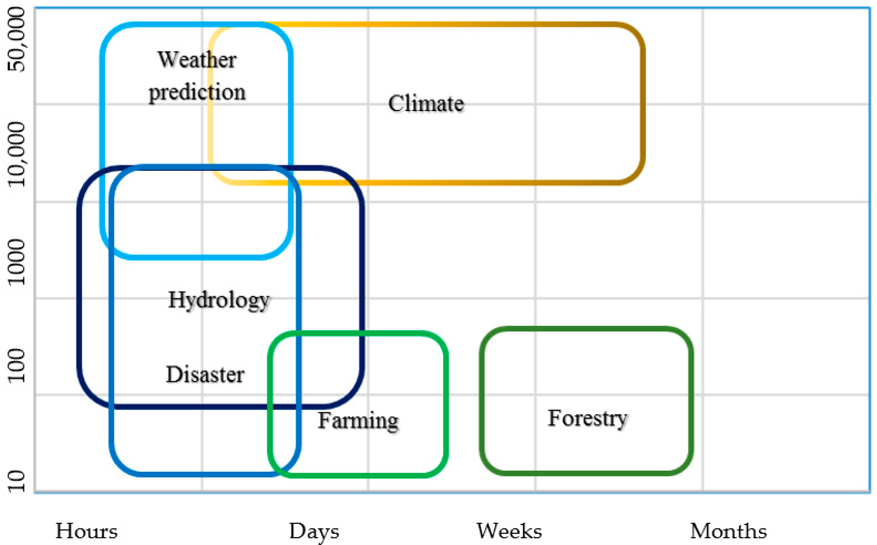
Microwave sensors have been successfully used to retrieve soil moisture. The advanced microwave scanning radiometer (AMSRE and AMSR2) [18], the advanced scatterometer (ASCAT) [19], soil moisture and ocean salinity (SMOS) [20], and soil moisture active passive (SMAP) [21] are among the microwave sensors that produce soil moisture products. Most of the above-mentioned soil moisture products have a coarse spatial resolution (>25 km) that is not suitable for agricultural purposes (Figure 1) [7,22,23].
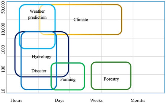
Figure 1.
Summary of spatial (m) and temporal resolution required for soil moisture application in different fields adopted from [15].
Active microwave data from the synthetic aperture radar (SAR) sensors can be operationally used to estimate SMC at high spatial resolution [24,25]. Due to the dramatic increase in the soil dielectric constant with an increase in water content and the high sensitivity of SAR data in X, L, or C band to the dielectric constant, radar microwave data can be used to estimate the SSM [16]. Gruber et al. (2013) investigated the potential of Sentinel-1 to capture local soil moisture variations with high radiometric accuracy by investigating the capability of the MetOp ASCAT data and Envisat ASAR [26]. The results showed that spatial soil moisture variations could not be captured by these coarse resolution SAR instruments. However, by launching the Sentinel-1A in 2014, a C-band SAR mission that was followed by Sentinel-1B in 2016, an unprecedented opportunity to obtain global 10–20 m SAR images and consequently SSM was provided for every 6–12 days. For instance, Bauer et al. (2018) presented a method to retrieve the global SSM from Sentinel-1 using a change detection algorithm based on a regression approach [27]. They used a dynamic Gaussian upscaling method to obtain an SSM map in 1 km spatial resolution. In the SSM estimation in 1 km, the method demonstrated its capability to measure soil moisture at high spatiotemporal resolution and thus has become particularly valuable when changes in local hydrology due to rain or irrigation have to be captured.
On the other hand, when the soil becomes moist, its color will be darkened and cooled, so using the optical/thermal image is also an attractive option for estimating SMC based on surface spectral reflectance [28,29,30,31] or surface temperature and thermal inertia [32]. An experiment was conducted in 2002 in a laboratory setting, looking at the reflected shortwave radiation (400–2500 nm) from four soil types at varying moisture contents [29]. The observed changes in soil reflectance showed a nonlinear relationship with moisture content that was described by an exponential model. In addition, if the SSM is expressed as the degree of saturation, the model is similar for different soil types [29]. Another study in 2019 investigated the soil surface response to the SSM variations using Landsat 8 images. A total of 103 samples of soil were analyzed using hyperspectral features, which indicated that SSM adversely affected soil reflectance, particularly within the NIR-SWIR region [31]. Launching Sentinel-2A in 2015, a mission of continuous earth observation, which was followed by Sentinel-2B in 2017, provided a potential solution to estimate SSM at high resolution. As proof, Yue et al., in 2019, developed indices for estimating bare soil moisture. These indices are made from differences in water absorption between shortwave-infrared and surface NDVI. This study concludes that the proposed SSM indices perform well when the SSM ranges between 0–0.5 but do not perform well when it reaches beyond 0.5 . Moreover, water absorption between shortwave-infrared bands is linear with SSM [33]. A study in 2020 investigated Sentinel-2 images to estimate SSM in rainfed and irrigated fields. It improved the spatial and temporal resolution of soil water content mapping by means of the optical trapezoid model driven by Sentinel-2. In this study, two scenarios were considered for optical trapezoid parameterization. The first scenario was based on a simple regression model to obtain the optical trapezoid parameters, and the second scenario determined the optical trapezoid parameters through a nonlinear model. The relationship between trapezoid parameters and SSM was investigated. They found that the nonlinear model better detects temporal and spatial soil moisture changes over different environments [34]. In addition, some studies have been conducted on the synergistic use of Sentinel-1 and Sentinel-2 imagery to take advantage of both satellites [24,25,35,36].
The virtue of mapping SSM in a high spatiotemporal resolution is becoming especially valuable when local hydrology changes due to rainfall or irrigation must be captured [27]. A study [8] illustrated that SSM estimation even in 1 km can quantify the impact of irrigation or rainfall in agricultural fields, which cannot be detected by downscaling soil moisture products from coarser sensors. Therefore, if the rainfall data are available, based on an inversion of soil water balance, high spatial SSM data can derive the amount of irrigation over agricultural lands [5,37,38].
In light of the above insight, although many studies tried to estimate SSM at the high spatial resolution, there is still a significant gap in estimating SSM in agricultural lands without additional data [8,39]. Therefore, this study focused on the agricultural domains with different crop types to propose a method to retrieve the SSM with reasonable accuracy.
This study first aims to answer the question of how SSM variations affect the soil surface spectral signature captured by Sentinel-2 and Sentinel-1 satellites over the agricultural domain. Second, it investigates which machine learning algorithm best estimates the SSM without the typical limitations on recent soil moisture maps (e.g., the spatial and temporal resolution). This method can be applied to any agricultural field since it is independent of other information such as soil type, crop type, land cover, and so forth. This method is sensitive to the effects of soil moisture variation on the surface response in electromagnetic waves.
The main objectives of the present study are as follows: (i) producing a soil moisture map based on Sentinel-2 images acquired over the five separate plantation zones; (ii) similarly, producing a soil moisture map based on Sentinel-1 images in the same study area; (iii) producing and comparing the generated soil map with ground measurements and SMAP-Sentinel1 1 km soil moisture product; and (iv) mapping the irrigated agriculture using the derived SSM data. The resulting soil moisture data can be used in irrigation scheduling and distinguishing the irrigated and rainfed agriculture.
2. Study Area and Dataset Description
2.1. Study Area
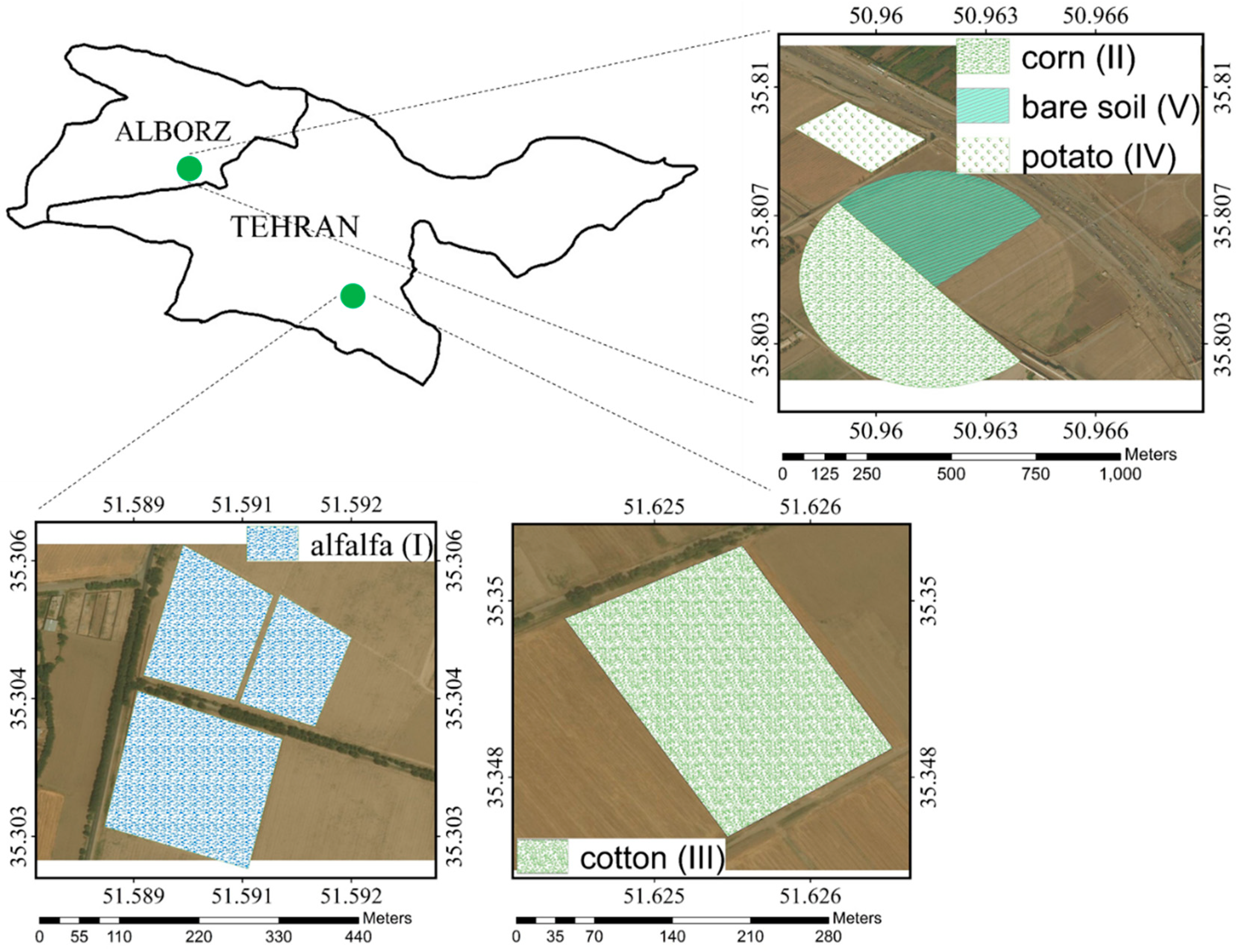
The study area consists of five farms located in Tehran and Alborz provinces in Iran. The total area of agricultural land is about 54 acres. Tehran farms use drip irrigation, while Alborz farms are equipped with a center pivot and sprinkler irrigation system. Figure 2 shows the location of the farms and the crop types.

Figure 2.
The location of the plantation fields in Tehran and Alborz provinces and a true color image of crop types in these fields.
Farms with different crop production were investigated for two main reasons: first, it is crucial to consider the soil texture and soil chemical/physical properties such as intrinsic soil color, soil roughness, and various local incident angles in agricultural fields; second, we planned to consider different plant growth stages [40] in our study. As the vegetation needed to be sparse enough (NDVI < 0.2) to prevent signal attenuation and soil surface coverage, the study was carried out in the early stages (sowing and emergence) of the crop’s growth cycle. The site specifications, location, and climate type with the number of field samples are presented in Table 2.
Table 2.
Characteristics of the soil sampling fields where the area name is defined as the name of the cultivated crop, followed by geographical area location, area, and the atmospheric model.
The average annual temperature in the study area is and the warmest month is July with an average temperature of . The region receives 244 mm of precipitation throughout the year. The study area land use map is shown in Figure 3.
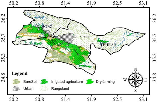
Figure 3.
Tehran and Alborz land use map.
2.2. Data Collection (Satellite Data and Ground Measurements)
2.2.1. Sentinel-1
Sentinel-1A and Sentinel-1B were launched in April 2014 and April 2016, respectively, as a part of the Copernicus program. Synthetic aperture radars (SAR) are indifferent to weather conditions and provide data in a dual- or single-polarization operation in the C-band (5.4 GHz) and interferometric wide (IW) swath mode. The Level-1 ground range detected (GRD) data from the SLC product with a spatial resolution of 10 m and revisit frequency of 6 days (3 days at the equator and less than one day at high latitudes) can be acquired from the sentinel-hub website (https://www.copernicus.eu/en, accessed on 10 October 2019).
GRD images in VV and VH polarization in ascending orbit (between 5 p.m. and 6 p.m. local time) are obtained according to Table 3.
Table 3.
Scheduling of the study site measurement campaigns and satellite passes.
2.2.2. Sentinel-2
The Sentinel-2 constellation is a land-monitoring mission developed by the European Space Agency (ESA), which comprises two satellites with multispectral imaging, Sentinel-2A and Sentinel-2B, launched in 2015 and 2017, respectively. The constellation provides global coverage with a revisit time of 5 days. The MSI sensor mounted on Sentinel-2 captures 13 spectral bands, from visible to short wave infrared (SWIR) at three different spatial resolutions (10, 20, and 60 m). To generate images with an equal spatial resolution in all bands, images were resampled to 10 m. The images were obtained from (https://www.copernicus.eu/en, accessed on 10 October 2019), which releases data in the “Level-2A” format. This product (Level-2A) includes radiometric, atmospheric, and cloud corrections, so no other processing is required [41].
The Sentinel-2 images are sensitive to weather conditions. Therefore, all ground samplings were performed in favorable weather conditions without any clouds. Regarding ground sampling days, several Level-2A images in descending orbit (between 11 a.m. and 12 a.m. local time) were taken according to Table 3.
2.2.3. Soil Moisture Active Passive (SMAP)
SMAP was launched in 2015 and planned to provide high-resolution global soil moisture data through the joint use of L-band radar and radiometer measurements. However, a few months into the mission, the radar became inoperable, and only the 36 km radiometer-based SSM product continued to provide global coverage every 2–3 days. The SMAP team used two approaches to retrieve the high-resolution capability of SMAP: (i) taking advantage of the overlapping radiometer footprint to create a higher resolution product (SMAP Enhanced 9 km) and (ii) combining SMAP radiometer measurements with an available SAR mission (i.e., Sentinel-1). In this study, the SMAP-Sentinel1 1 km product [42] is used as a satellite product reference to compare with SSM-S1 and SSM-S2 data (https://search.earthdata.nasa.gov, accessed on 10 October 2019).
2.2.4. Ground Measurements
For ground sampling, agricultural fields were classified according to their crop type. Sampling was performed when the plants were in the early stages of growth (NDVI < 0.2), so the surface was not covered with plants. After the soil surface was cleaned, the samples were taken from a depth of about 10 cm. In total, 170 samples (110 samples for multispectral images and 60 samples for SAR images) were taken. The samples’ gravimetric soil moisture content was obtained using the drying process in the laboratory depicted in Figure 4. By measuring the soil density, the volumetric soil moisture was also calculated. The calculated moisture represented the average SSM of the corresponding pixel.
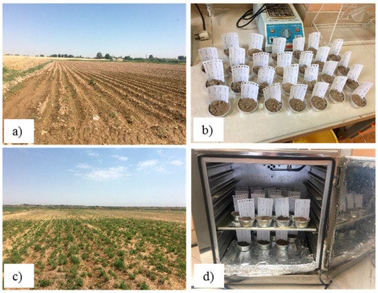
Figure 4.
The process of measuring the volumetric soil moisture at sites. (a,c) shows the fields and (b,d) shows the soil samples.
3. Methodology
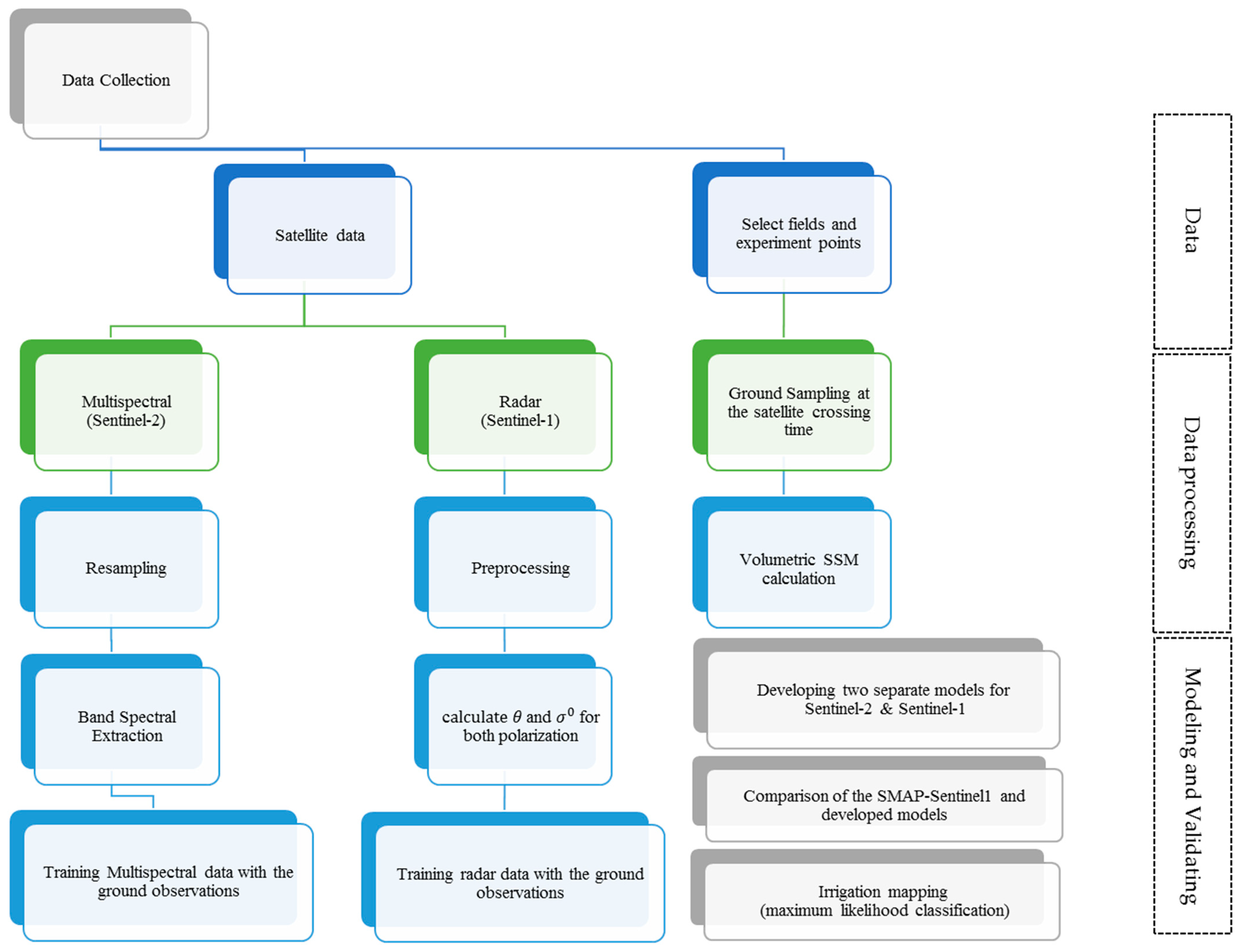
As described before, this study investigates the soil spectral response to SSM variation over irrigated agriculture. For this purpose, a semi-empirical model was established to estimate the SSM. The modeling process is shown in Figure 5.

Figure 5.
The flowchart of the present method to retrieve surface soil moisture based on multispectral and microwave data.
3.1. Soil Multi-Spectral Response
Sentinel-2 Images
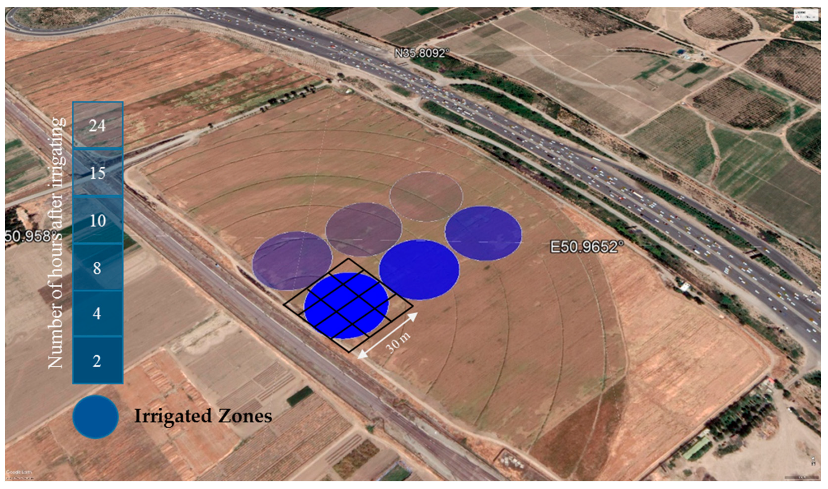
This stage aims to develop a semi empirical model based on Sentinel-2 imagery. The inputs of the model include the soil surface reflectance in different bands captured by Sentinel-2 and the crop type. The output of the model is the SSM as illustrated in Equation (1). The model assumes that since all conditions (e.g., soil texture, vegetation cover, product type, and so forth) remain constant in each field sampling, changes in the soil surface reflectance must be related to the SSM difference. Therefore, the first step is to define the driest pixel and put it as the base pixel (BP). By comparing the BP with other samples, the influence of the SSM on soil surface response could be investigated, and this relationship could be modeled, assisted by machine learning algorithms. This model would be more accurate if the training samples covered all possible soil moisture content values. An experiment was designed to irrigate the field (V) at different times before the satellite overpass to train the model with a wide variety of SSM. Each circle was watered by a sprinkler 2, 4, 8, 10, 15, and 24 h before the satellite overpass, and the closer start time corresponded with a wetter soil state.
Consequently, different SSM zones were created at the time of satellite overpass, as shown in Figure 6. Since each sprinkler can water a circle with a radius of 15 m, each zone consists of nine Sentinel-2 pixels that are entirely or partially bounded by the sprinkler circle (Figure 6). Therefore, due to the conditions, the results show how surface reflectance is affected by SSM.

Figure 6.
The experimental design to make different irrigated zones. Each circle was watered by a sprinkler 2, 4, 8, 10, 15, and 24 h before the satellite passed as described in the legend. The transparency indicates the amount of SSM during the satellite’s passage (lower transparency corresponded with lower SSM content).
This procedure was repeated for other study fields as well. Overall, 110 different soil samples were collected during the field campaign’s specific days mentioned in Table 3. From this point on, the soil moisture obtained by this method is called SSM-S2.
3.2. Soil Backscatter Response
Sentinel-1 Image
A semi empirical model is established based on Sentinel-1 images. Since all circumstances such as surface roughness, soil properties, surface features, and radar properties remain constant in each sampling of each field, the model assumes that the SSM is a function of the surface backscatter in both vertical () and horizontal () polarization and the local incident angle (), as described in Equation (2). Therefore, the surface backscatter in vertical and horizontal polarization and the local incident angle were used as input and the SSM is used as the output of the model. Additionally, to consider the effect of the vegetation cover and soil conditions, we defined a polarization ratio () and graphed this relationship. As this model is based on the Sentinel-1 images, it is called SSM-S1. For SSM-S1 training, 60 points were sampled to investigate the influence of the SSM on input parameters ().
Preprocessing the Sentinel-1 images, according to the ESA statement, the GRD products preprocessing has some steps include applying orbit file, thermal noise removal, calibration, speckle filtering, Range Doppler Terrain Correction, and conversion to dB. As the last step of the preprocessing workflow, the unitless backscatter coefficient is converted to dB using a logarithmic transformation.
3.3. Soil Moisture Retrieval and Validation
Three machine learning algorithms, including multilayer perceptron (MLP), convolutional neural network (CNN), and linear regression, were used to estimate SSM from Sentinel-1 and Sentinel-2 retrieval. Studies showed that MLP has the ability to solve a complex problem such as fitness approximation [43]. The CNN algorithm is similar to MLP, except that it can recognize spatial relations by taking a tensor instead of a vector as the input. Linear regression is a supervised learning algorithm that predicts a dependent variable value based on some given independent variables. These algorithms were used to create a relationship between features and targets. Each algorithm used 80% of the data for training and 20% for validating the model performance (training and validating data were selected randomly). For validating the model, the estimated SSM was compared with ground measurements. This process was repeated 100 times, and the RMSEs were reported. Since CNN has the best performance among other algorithms, it is applied to estimate SSM in optical and radar images.
3.4. Comparison of the SMAP Soil Moisture and Proposed SSM
Although the validity of the model was verified using ground data, this section aims to compare the result of the proposed method with the currently available high-resolution soil moisture product (SMAP-Sentinel1). The spatial resolution of SMAP-Sentinel1 soil moisture is 1 km, while proposed methods retrieve the SSM at 10 m resolution. Nevertheless, it will be possible to investigate the changes in SSM over time for a given area. To compare the performance of SMAP-Sentinel1 and SSM-S1 and SSM-S2 soil moisture products, two study areas consisting of the agricultural fields (II and V) were selected, and the time series of SSM was compared from 1 January 2019 to 1 January 2020. As SMAP went into safe mode in two months of 2019 (June and July), no data were collected during this period. In Sentinel-2 images, a cloud filter was applied in the Google Earth Engine, and dates with more than 20% of cloud coverage were removed from the analysis. Moreover, we choose not to run the SSM-S2 algorithm during the growing season (NDVI > 0.2) due to the ground coverage [40].
3.5. Image Classification
A pixel-based classification method (unsupervised classification) was used to cluster similar pixels into specific groups without requiring the user to provide sample classes. For this purpose, maximum likelihood classification was applied to the SSM result into four classes: urban, dry farming, rangeland, and irrigated agriculture. This classification was performed only based on changes in surface soil moisture to identify irrigated agriculture. The overall accuracy, kappa index, and commission and omission error are reported for the classified map.
4. Results and Discussion
4.1. Sentinel-2 Multispectral Response of SSM
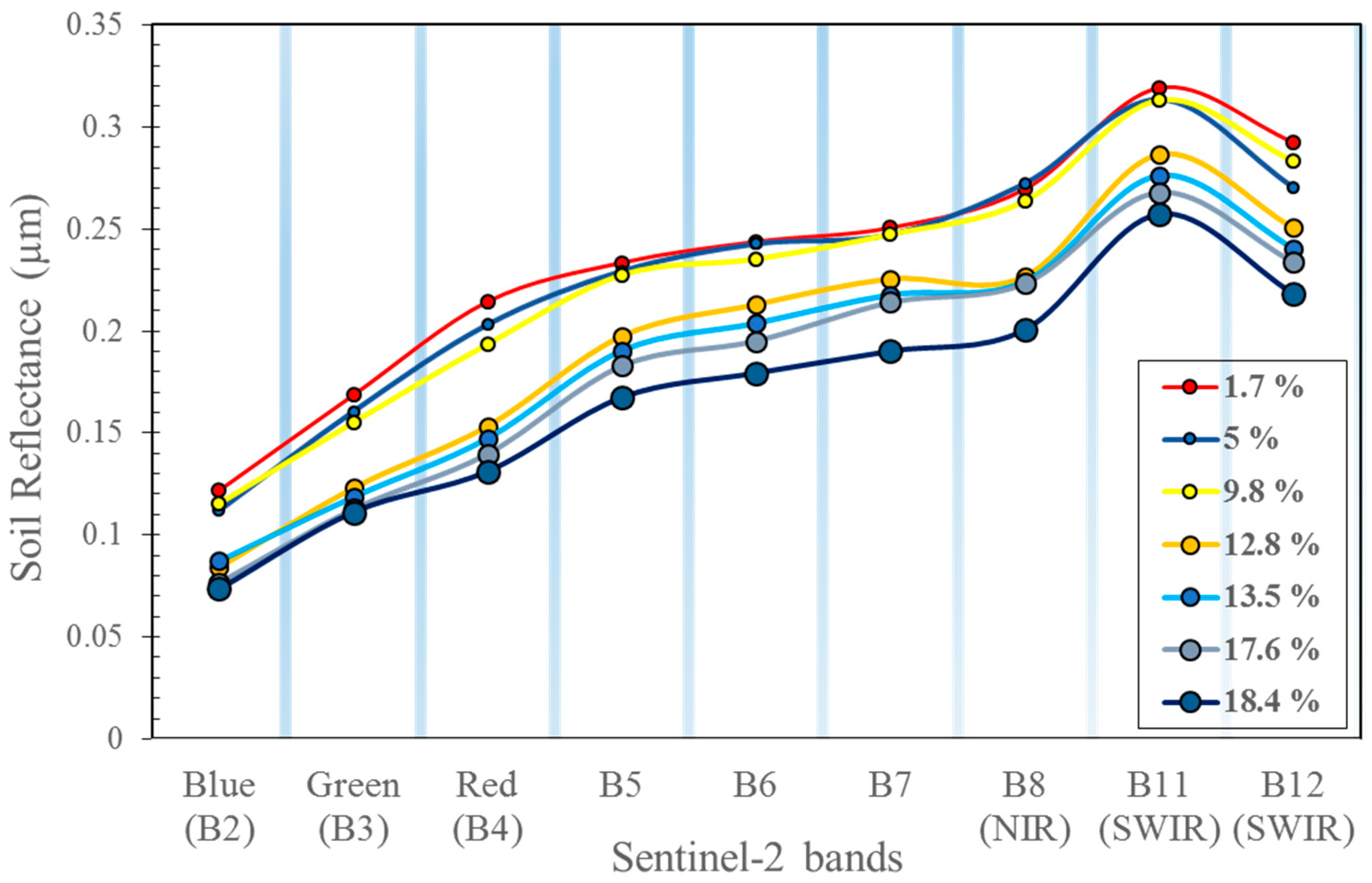
The soil surface reflectance captured by Sentinel-2 is highly dependent on SSM, as depicted in Figure 7. Indeed, when SSM increases, the soil color darkens and the soil reflectance decreases [44]. Although reflectance in all the Sentinel-2 bands decreases with increasing soil moisture, the visible bands B2 (blue), B3 (green), and B4 (red) have the highest negative correlation with the SSM (R < −0.76). However, previous studies showed that the longer wavelengths are more sensitive to the SSM variation if it increases more than 0.2 [29]. Since, in irrigation events, the SSM is almost about 0.2 due to drainage and evapotranspiration processes, Sentinel-2 bands are a good choice for SSM estimation. Moreover, it is possible to monitor soil moisture at high resolution using multispectral cameras mounted on drones or UAVs over agricultural fields [45].
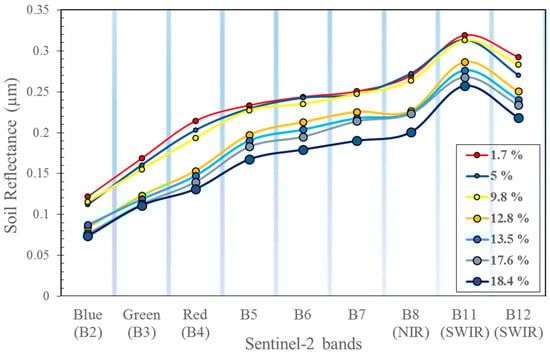
Figure 7.
Higher SSM decreases the soil surface reflectance at the different bands of Sentinel-2 over an agricultural area (I, II, III, IV, and V). Different colors indicate different soil moisture levels, and larger markers indicate higher soil moisture levels.
4.2. Sentinel-1 Backscatter Response of SSM
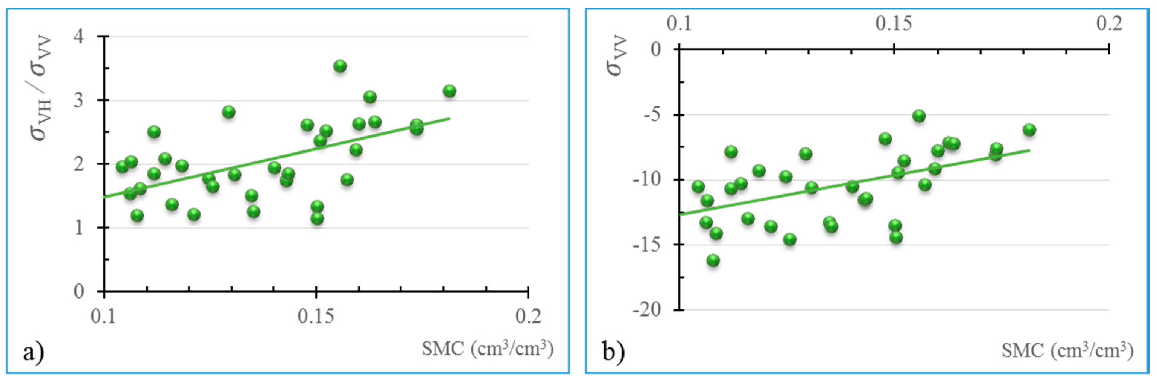
One of the factors that affect the surface backscatter is the amount of soil moisture content. Higher backscatter is observed by increasing the SSM [46]. In low soil moisture content, other factors such as soil roughness affect the surface backscatter. Therefore, to eliminate other factors, graphs are plotted for SSM greater than 0.05 [47]. For better presentation, the results are depicted in two separated graphs; the first is versus soil moisture and the second is versus soil moisture as depicted in Figure 8. Dual polarized images ( or ) help to better understand the relationship of soil moisture and surface backscatter since this PR is sensitive to surface features and considers the effect of vegetation and soil conditions [48]. Figure 8a presented radar versus soil moisture, and Figure 8b illustrated the versus soil moisture. Moreover, it can be concluded from these two graphs that increases at a higher rate relative to the by increasing the soil moisture.
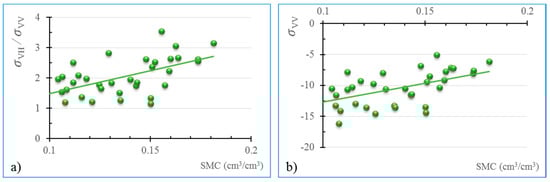
Figure 8.
An increase in the SSM increases horizontal and vertical backscatter. (a) Backscatter ratio of horizontal to vertical () polarization. (b) Vertical polarization ().
4.3. Validation of the Proposed Method
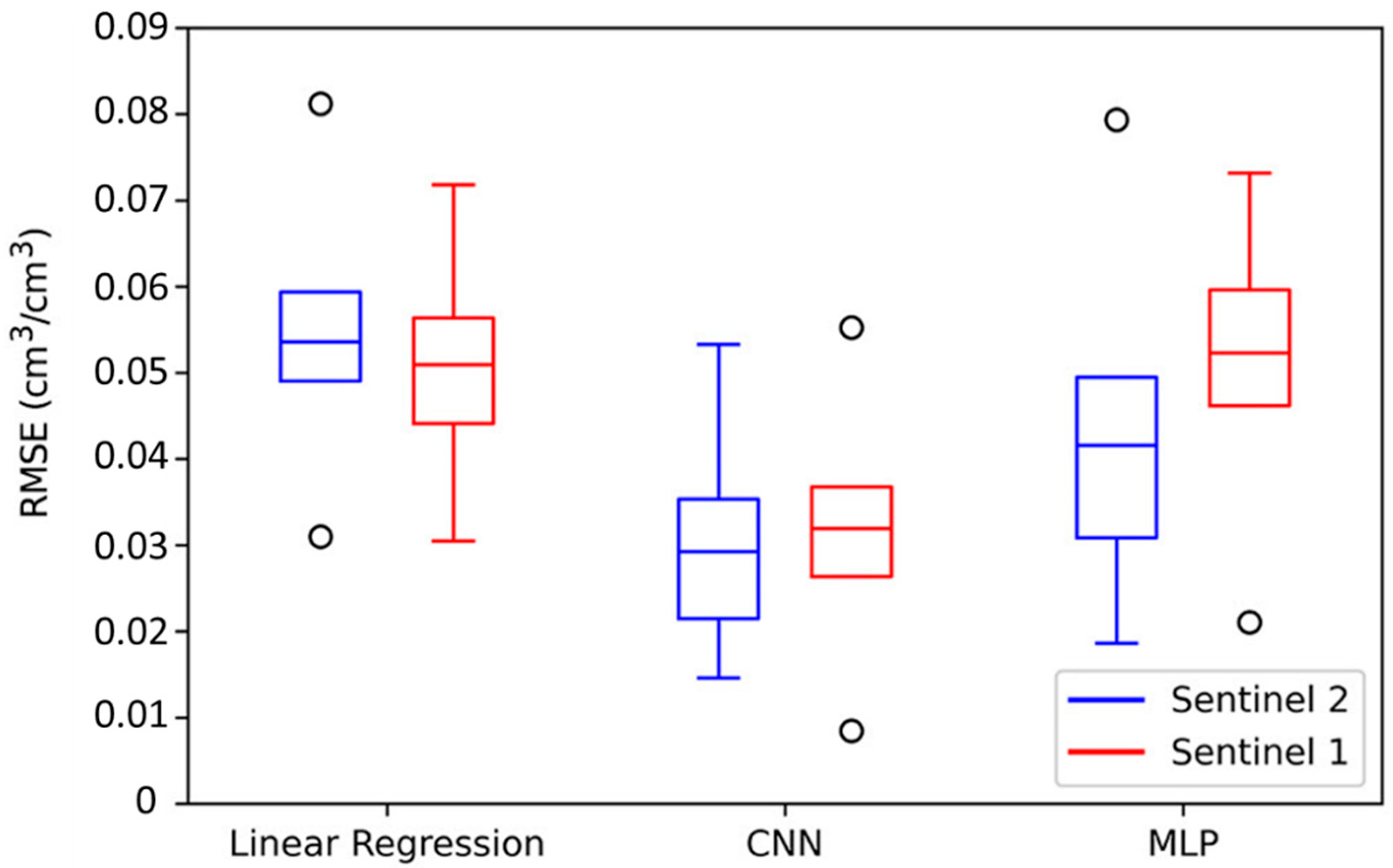
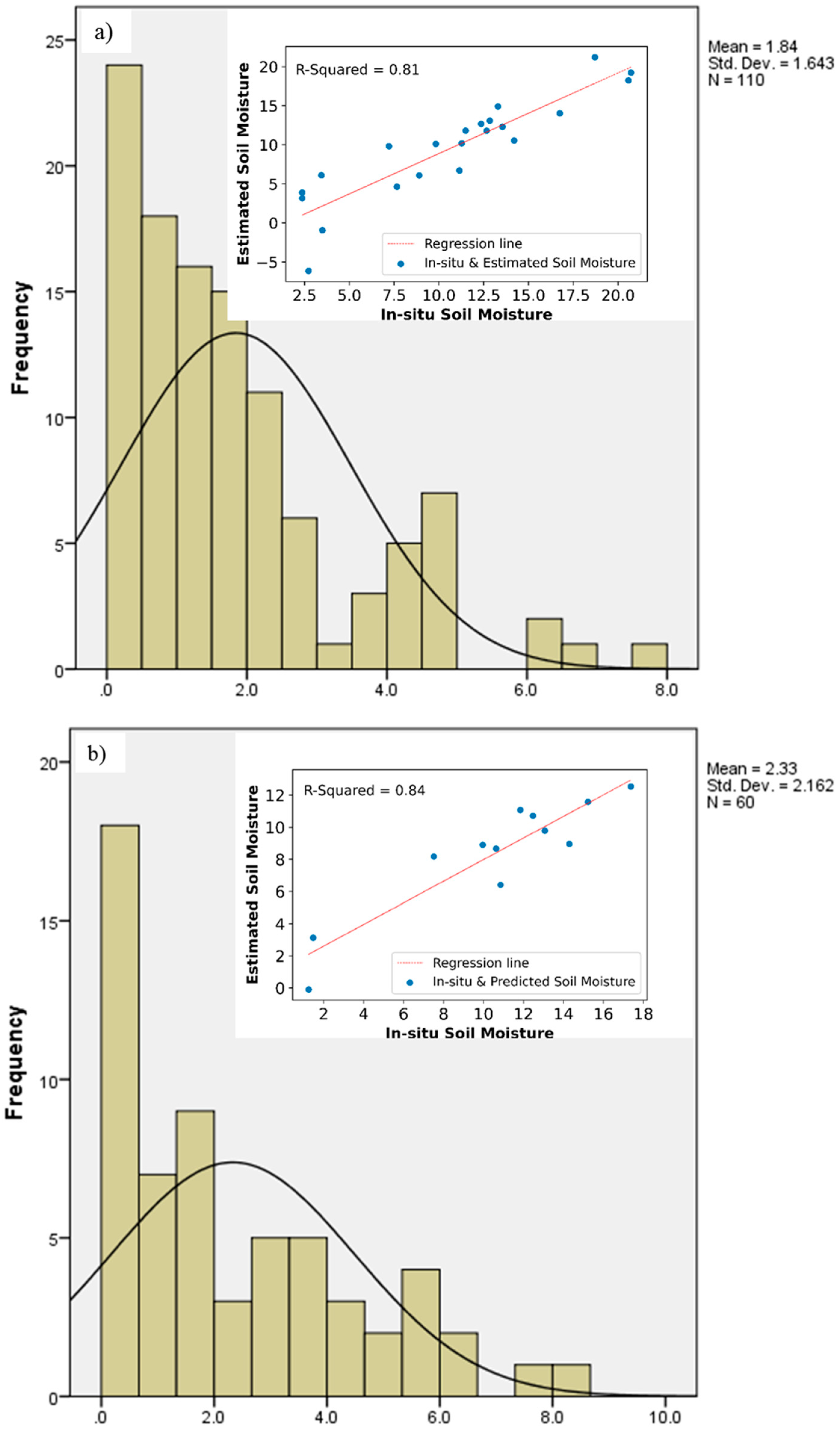
The relationship between the SSM and satellite imagery is a very complex relationship. The one-way analysis of variance (ANOA) illustrated that there is a linear (p < 0.001) or nonlinear (p < 0.021) relationship between SSM and soil reflectance. However, Figure 9 shows deep learning algorithms perform better than the multiple regression analysis. Among deep learning algorithms, CNN is performing better than MLP as it considers the nearby pixels to understand spatial relationships. The mean value of RMSE in the CNN algorithm was for multispectral images and for radar data. Figure 10 shows the validation of the multispectral and radar images separately. Moreover, the model errors (residuals) distribution calculated by computing the absolute difference between ground measurement and the estimated SSM is shown.
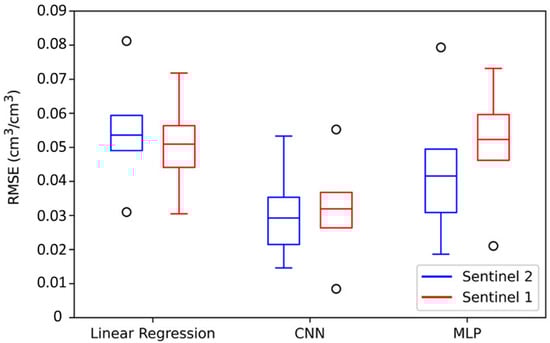
Figure 9.
The comparison of three different machine learning algorithms developed by SSM-S1 and SSM-S2. Each plot shows the statistics of RMSE results in 100 runs. Hollow circles show the outlier.
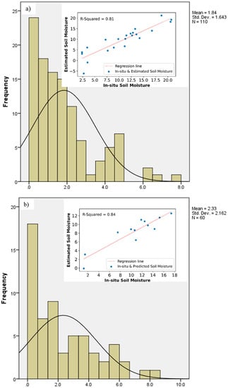
Figure 10.
Soil moisture was retrieved by the proposed method as a function of soil moisture measured in the reference fields. (a) Soil moisture retrieved by multispectral images of Sentinel-2; the mean RMSE is and model error distribution. (b) Soil moisture retrieved by radar images of Sentinel-1; the mean RMSE is and model error distribution of radar images.
4.4. Comparison of the SMAP and Proposed SSM Models
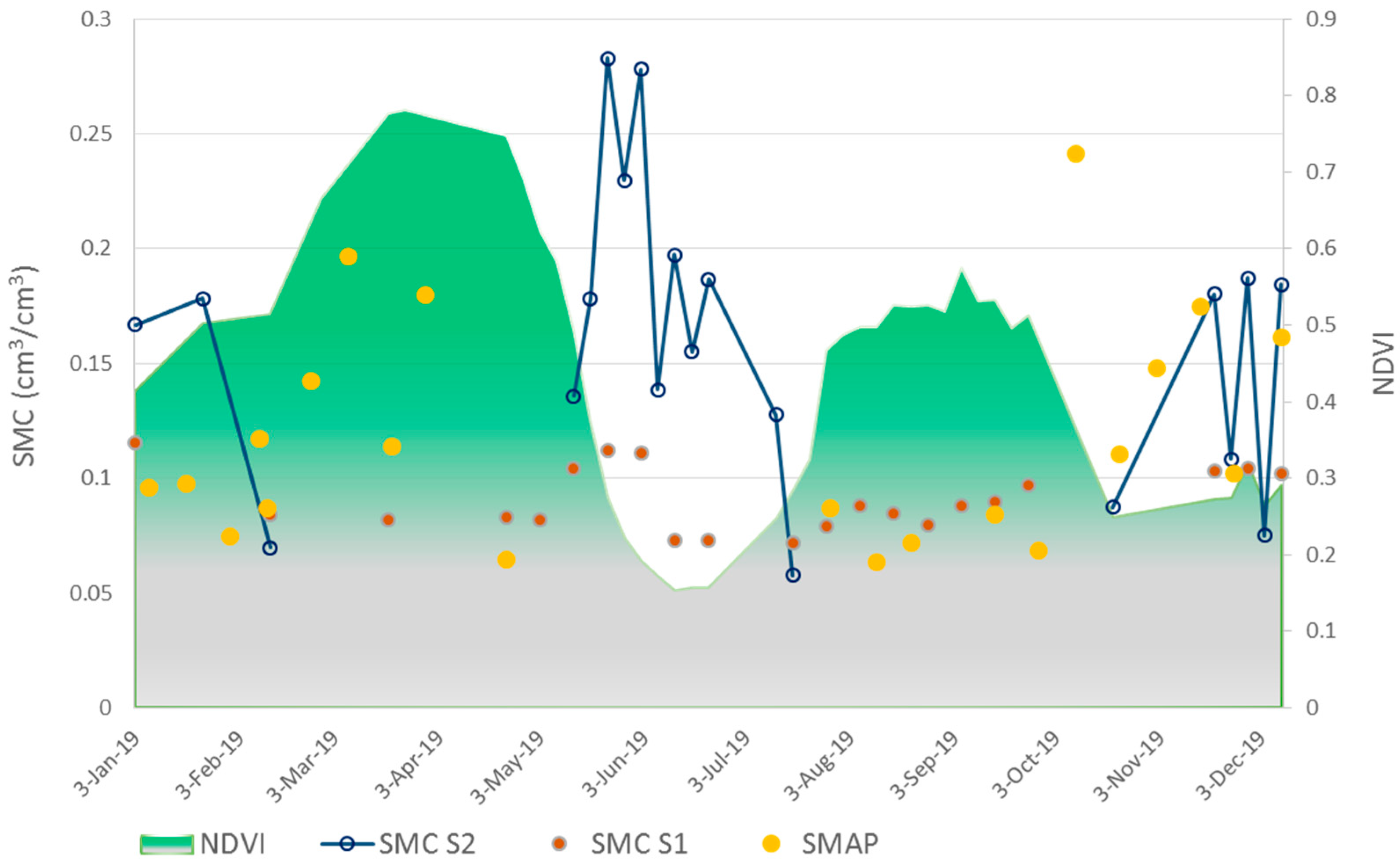
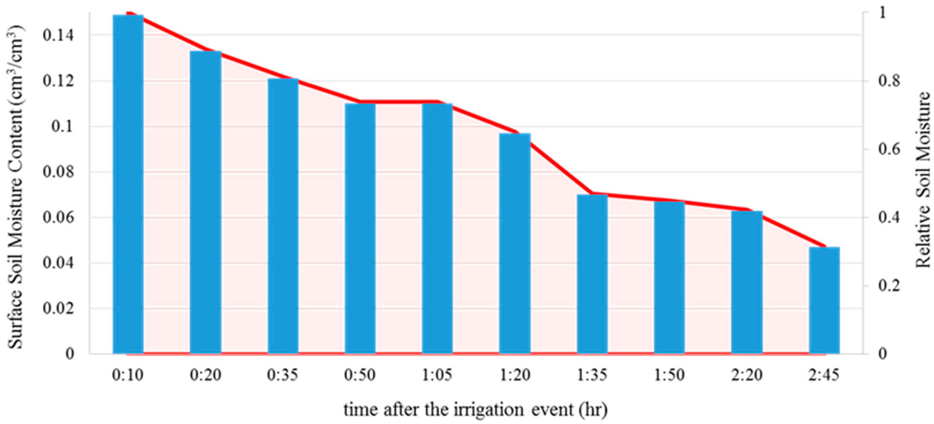
Since there is a spatial mismatch between the SMAP-Sentinel1 (1 km) and Sentinel 1 and 2 (10 m) SSM products, and the machine learning algorithm only trained over the case study plots, we choose to compare the SMAP-Sentinel1 with SSM-S1 and SSM-S2 temporally rather than spatially according to Figure 11. As illustrated in this figure, the SSM-S1 is in better agreement with the SMAP-Sentinel1 relative to the SSM-S2. The SMAP-Sentinel1 uses an L-band radiometer, which is less affected by the dense vegetation compared to the Sentinel-1 radar that operates in the C band. This explains the significant difference in SSM estimation (March to May) by Sentinel-1 and SMAP-Sentinel1. The SSM-S2 model is susceptible to surface coverage, especially after the plant’s germination. Thus, when the NDVI is greater than 0.2, this algorithm could not work properly, and we masked the data. The acquisition time of Sentinel-2 is about 11:16 a.m, but the acquisition time of Sentinel-1 is about 5:37 p.m. According to the study mentioned in the introduction section ([49]), although the soil moisture from a rain event can be observed up to 3 days after rainfall, the situation is different in irrigation events. The rate and the time of irrigating are less than the rainfall. Runoff and puddling are rarely observed in irrigating, so the root zone layer is less likely to be saturated. Moreover, on rainy days, the weather is mostly cloudy and the temperature is low. So the evaporation rate after rainfall is much lower than the evaporation rate after an irrigation event. In our region, due to percolation and evapotranspiration processes, the surface soil moisture becomes dry entirely in less than 24 h. We examined this using a sprinkler that irrigated a part of the land for about one hour. After that, the soil moisture was measured at a specific point near the sprinkler every 15 min. As Figure 12 shows, The SSM began to decrease after irrigation stopped and after about 3 h, it lost about 70% of its moisture. Therefore, as most of the irrigation occurred in the morning and the soil begins to dry out in the evening, the SSM-S2 shows an entirely different time series from the SSM derived from Sentinel-1 or SMAP.

Figure 11.
Time series of estimated SSM by SMAP-Sentinel1, SSM-S1, and SSM-S2 over plots II and V.

Figure 12.
Time series of surface soil moisture in a point located near a sprinkler after the irrigation stopped.
4.5. Locating Agricultural Area with SMC Classification
SSM-S1 and SSM-S2 are used to detect the irrigated area using unsupervised classification. As illustrated in Figure 13, farms are detected in irrigated agriculture and dry farming classes; moreover, the city area is recognized as well. To better understand this classification, an aerial true-color image of the same place and the same time is derived from google earth images depicted beside the classification. The overall accuracy is 77% the kappa coefficient is 65%, and the commission error for detecting irrigated agriculture is 56%.
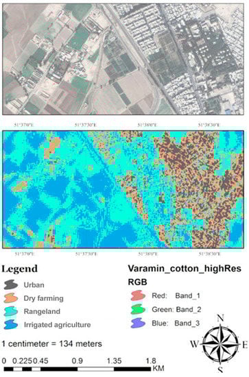
Figure 13.
Land use classification based on Sentinel-2 SSM-S2 algorithm.
5. Conclusions
This study aims to produce a soil moisture map at a high spatial resolution applicable for agricultural monitoring at a plot scale. This estimation was performed using Sentinel-1 (SSM-S1) and Sentinel-2 (SSM-S2) satellite imagery. This study showed the CNN machine learning algorithm could estimate the SSM precisely. The RMSE is in SSM-S1 and in SSM-S2 data. Thus, Sentinel-1 images are more suitable for estimating soil moisture.
In the second part of the study, we found that the proposed SSM product is in good agreement with the SMAP-Sentinel1 soil moisture product. The derived SSM is also used to classify the irrigated and non-irrigated areas. To achieve that, an unsupervised classification was implemented on the soil moisture map and clustered the area into four classes (urban, dry farming, rangeland, and irrigated agricultural area) with an overall accuracy of 76%.
This study shows the ability to detect the irrigated agriculture from rainfed agriculture. Moreover, it is possible to detect the irrigated agriculture based on the SSM spatial variation up to 7 h after irrigation in a semi-arid region. With this results, the number of irrigation events on agricultural lands could be identified if the optical images are received in less than daily temporal resolution. As this study can map the SSM in high resolution, future work will involve implementing this method to quantify irrigation amounts over the agricultural area at plot scale.
Author Contributions
Conceptualization, E.J., S.R. and M.T.; methodology, S.R., E.J. and M.T.; software, S.R.; validation, S.R. and E.J.; formal analysis, S.R.; resources, M.T.; data curation, S.R.; writing-original draft preparation, S.R.; writing—review and editing, S.R. and E.J.; visualization, S.R. and E.J.; Supervision, M.T. and E.J.; project administration, M.T.; funding acquisition, M.T. All authors have read and agreed to the published version of the manuscript.
Funding
The authors would like to acknowledge Sharif University of Technology civil and environmental engineering faculty for providing financial support for this project.
Institutional Review Board Statement
Not applicable.
Informed Consent Statement
Not applicable.
Data Availability Statement
The data presented in this study are available on request from the corresponding author.
Acknowledgments
The research was carried out in University of Tehran agriculture research farms. The authors would like to thank the following people for helping us with this project; Goldansaz, Jahansuz, and Rafiei, whose collaboration greatly enhanced the data collection procedure. In addition, the authors wish to acknowledge the help provided by the technical and support staff in the environmental science laboratory of the Sharif University of Technology.
Conflicts of Interest
The authors declare no conflict of interest.
References
- Robock, A.; Vinnikov, K.Y.; Srinivasan, G.; Entin, J.K.; Hollinger, S.E.; Speranskaya, N.A.; Liu, S.; Namkhai, A. The Global Soil Moisture Data Bank. Bull. Am. Meteorol. Soc. 2000, 81, 1281–1299. [Google Scholar] [CrossRef] [Green Version]
- Verstraeten, W.W.; Veroustraete, F.; Feyen, J. Assessment of evapotranspiration and soil moisture content across different scales of observation. Sensors 2008, 8, 70–117. [Google Scholar] [CrossRef] [PubMed] [Green Version]
- Seneviratne, S.I.; Corti, T.; Davin, E.L.; Hirschi, M.; Jaeger, E.B.; Lehner, I.; Orlowsky, B.; Teuling, A.J. Investigating soil moisture–climate interactions in a changing climate: A review. Earth-Science Rev. 2010, 99, 125–161. [Google Scholar] [CrossRef]
- Tuttle, S.E.; Salvucci, G.D. A new approach for validating satellite estimates of soil moisture using large-scale precipitation: Comparing AMSR-E products. Remote Sens. Environ. 2014, 142, 207–222. [Google Scholar] [CrossRef]
- Jalilvand, E.; Tajrishy, M.; Alsadat, S.; Zadeh, G.; Brocca, L. Remote Sensing of Environment Quantification of irrigation water using remote sensing of soil moisture in a semi-arid region. Remote Sens. Environ. 2019, 231, 111226. [Google Scholar] [CrossRef]
- Panhwar, Q.A.; Ali, A.; Naher, U.A.; Memon, M.Y. Fertilizer management strategies for enhancing nutrient use efficiency and sustainable wheat production. In Organic Farming; Elsevier: Amsterdam, The Netherlands, 2019; pp. 17–39. [Google Scholar]
- Mulla, D.J. Twenty five years of remote sensing in precision agriculture: Key advances and remaining knowledge gaps. Biosyst. Eng. 2013, 114, 358–371. [Google Scholar] [CrossRef]
- Brocca, L.; Tarpanelli, A.; Filippucci, P.; Dorigo, W.; Zaussinger, F.; Gruber, A.; Fernández-Prieto, D. How much water is used for irrigation? A new approach exploiting coarse resolution satellite soil moisture products. Int. J. Appl. earth Obs. Geoinf. 2018, 73, 752–766. [Google Scholar] [CrossRef]
- Zaussinger, F.; Dorigo, W.; Gruber, A.; Tarpanelli, A.; Filippucci, P.; Brocca, L. Estimating irrigation water use over the contiguous United States by combining satellite and reanalysis soil moisture data. Hydrol. Earth Syst. Sci. 2019, 23, 897–923. [Google Scholar] [CrossRef] [Green Version]
- Pratola, C.; Barrett, B.; Gruber, A.; Dwyer, E. Quality assessment of the CCI ECV soil moisture product using ENVISAT ASAR wide swath data over Spain, Ireland and Finland. Remote Sens. 2015, 7, 15388–15423. [Google Scholar] [CrossRef] [Green Version]
- Zacharias, S.; Bogena, H.; Samaniego, L.; Mauder, M.; Fuß, R.; Pütz, T.; Frenzel, M.; Schwank, M.; Baessler, C.; Butterbach-Bahl, K. A network of terrestrial environmental observatories in Germany. Vadose Zo. J. 2011, 10, 955–973. [Google Scholar] [CrossRef] [Green Version]
- Smith, A.B.; Walker, J.P.; Western, A.W.; Young, R.I.; Ellett, K.M.; Pipunic, R.C.; Grayson, R.B.; Siriwardena, L.; Chiew, F.H.S.; Richter, H. The Murrumbidgee soil moisture monitoring network data set. Water Resour. Res. 2012, 48. [Google Scholar] [CrossRef]
- Evans, J.G.; Ward, H.C.; Blake, J.R.; Hewitt, E.J.; Morrison, R.; Fry, M.; Ball, L.A.; Doughty, L.C.; Libre, J.W.; Hitt, O.E. Soil water content in southern England derived from a cosmic-ray soil moisture observing system–COSMOS-UK. Hydrol. Process. 2016, 30, 4987–4999. [Google Scholar] [CrossRef] [Green Version]
- Wang, L.; Qu, J.J. Satellite remote sensing applications for surface soil moisture monitoring: A review. Front. Earth Sci. China 2009, 3, 237–247. [Google Scholar] [CrossRef]
- Peng, J.; Albergel, C.; Balenzano, A.; Brocca, L.; Cartus, O.; Cosh, M.H.; Crow, W.T.; Dabrowska-Zielinska, K.; Dadson, S.; Davidson, M.W.J. A roadmap for high-resolution satellite soil moisture applications–confronting product characteristics with user requirements. Remote Sens. Environ. 2020, 112162. [Google Scholar]
- Baghdadi, N.; Camus, P.; Beaugendre, N.; Issa, O.M.; Zribi, M.; Desprats, J.F.; Rajot, J.L.; Abdallah, C.; Sannier, C. Estimating surface soil moisture from TerraSAR-X data over two small catchments in the Sahelian Part of Western Niger. Remote Sens. 2011, 3, 1266–1283. [Google Scholar] [CrossRef] [Green Version]
- Srivastava, P.K. Satellite soil moisture: Review of theory and applications in water resources. Water Resour. Manag. 2017, 31, 3161–3176. [Google Scholar] [CrossRef]
- Njoku, E.G.; Jackson, T.J.; Lakshmi, V.; Chan, T.K.; Nghiem, S. V Soil moisture retrieval from AMSR-E. IEEE Trans. Geosci. Remote Sens. 2003, 41, 215–229. [Google Scholar] [CrossRef]
- Wagner, W.; Hahn, S.; Kidd, R.; Melzer, T.; Bartalis, Z.; Hasenauer, S.; Figa-Saldana, J.; De Rosnay, P.; Jann, A.; Schneider, S. The ASCAT soil moisture product: A review of its specifications, validation results, and emerging applications. Meteorol. Z. 2013. [Google Scholar] [CrossRef] [Green Version]
- Kerr, Y.H.; Waldteufel, P.; Richaume, P.; Wigneron, J.P.; Ferrazzoli, P.; Mahmoodi, A.; Al Bitar, A.; Cabot, F.; Gruhier, C.; Juglea, S.E. The SMOS soil moisture retrieval algorithm. IEEE Trans. Geosci. Remote Sens. 2012, 50, 1384–1403. [Google Scholar] [CrossRef]
- Entekhabi, D.; Njoku, E.G.; O’Neill, P.E.; Kellogg, K.H.; Crow, W.T.; Edelstein, W.N.; Entin, J.K.; Goodman, S.D.; Jackson, T.J.; Johnson, J. The soil moisture active passive (SMAP) mission. Proc. IEEE 2010, 98, 704–716. [Google Scholar] [CrossRef]
- Nandurkar, S.R.; Thool, V.R.; Thool, R.C. Design and development of precision agriculture system using wireless sensor network. In Proceedings of the 2014 First International Conference on Automation, Control, Energy and Systems (ACES), Hooghly, India, 1–2 February 2014; pp. 1–6. [Google Scholar]
- Domínguez-Niño, J.M.; Oliver-Manera, J.; Girona, J.; Casadesús, J. Differential irrigation scheduling by an automated algorithm of water balance tuned by capacitance-type soil moisture sensors. Agric. Water Manag. 2020, 228, 105880. [Google Scholar] [CrossRef]
- Gao, Q.; Zribi, M.; Escorihuela, M.J.; Baghdadi, N. Synergetic use of sentinel-1 and sentinel-2 data for soil moisture mapping at 100 m resolution. Sensors (Switzerland) 2017, 17. [Google Scholar] [CrossRef] [PubMed] [Green Version]
- Foucras, M.; Zribi, M.; Baghdadi, N. Estimating 500-m Resolution Soil Moisture Using. Water 2020, 12, 866. [Google Scholar] [CrossRef] [Green Version]
- Gruber, A.; Wagner, W.; Hegyiova, A.; Greifeneder, F.; Schlaffer, S. Potential of Sentinel-1 for high-resolution soil moisture monitoring. In Proceedings of the 2013 IEEE International Geoscience and Remote Sensing Symposium-IGARSS, 2013, Melbourne, Australia, 21–26 July 2013; pp. 4030–4033. [Google Scholar]
- Bauer-Marschallinger, B.; Freeman, V.; Cao, S.; Paulik, C.; Schaufler, S.; Stachl, T.; Modanesi, S.; Massari, C.; Ciabatta, L.; Brocca, L. Toward global soil moisture monitoring with Sentinel-1: Harnessing assets and overcoming obstacles. IEEE Trans. Geosci. Remote Sens. 2018, 57, 520–539. [Google Scholar] [CrossRef]
- Muller, E.; Decamps, H. Modeling soil moisture–reflectance. Remote Sens. Environ. 2001, 76, 173–180. [Google Scholar] [CrossRef] [Green Version]
- Lobell, D.B.; Asner, G.P. Moisture effects on soil reflectance. Soil Sci. Soc. Am. J. 2002, 66, 722–727. [Google Scholar] [CrossRef]
- Kaleita, A.L.; Tian, L.F.; Hirschi, M.C. Relationship between soil moisture content and soil surface reflectance. Trans. ASAE 2005, 48, 1979–1986. [Google Scholar] [CrossRef] [Green Version]
- Thi, D.N.; Ha, N.T.T.; Dang, Q.T.; Koike, K.; Trong, N.M. Effective band ratio of landsat 8 images based on VNIR-SWIR reflectance spectra of topsoils for soil moisture mapping in a tropical region. Remote Sens. 2019, 11. [Google Scholar] [CrossRef] [Green Version]
- Lakshmi, V.; Jackson, T.J.; Zehrfuhs, D. Soil moisture–temperature relationships: Results from two field experiments. Hydrol. Process. 2003, 17, 3041–3057. [Google Scholar] [CrossRef]
- Yue, J.; Tian, J.; Tian, Q.; Xu, K.; Xu, N. Development of soil moisture indices from differences in water absorption between shortwave-infrared bands. Isprs J. Photogramm. Remote Sens. 2019, 154, 216–230. [Google Scholar] [CrossRef]
- Ambrosone, M.; Matese, A.; Di Gennaro, S.F.; Gioli, B.; Tudoroiu, M.; Genesio, L.; Miglietta, F.; Baronti, S.; Maienza, A.; Ungaro, F. Retrieving soil moisture in rainfed and irrigated fields using Sentinel-2 observations and a modified OPTRAM approach. Int. J. Appl. Earth Obs. Geoinf. 2020, 89, 102113. [Google Scholar] [CrossRef]
- Attarzadeh, R.; Amini, J.; Notarnicola, C.; Greifeneder, F. Synergetic use of Sentinel-1 and Sentinel-2 data for soil moisture mapping at plot scale. Remote Sens. 2018, 10, 1285. [Google Scholar] [CrossRef] [Green Version]
- Bousbih, S.; Zribi, M.; El Hajj, M.; Baghdadi, N.; Chabaane, Z.L.; Fanise, P.; Boulet, G. Sentinel-1 and Sentinel-2 data for soil moisture and irrigation mapping over semi-arid region. In Proceedings of the IGARSS 2019-2019 IEEE International Geoscience and Remote Sensing Symposium, Yokohama, Japan, 28 July–2 August 2019; pp. 7022–7025. [Google Scholar]
- Filippucci, P.; Tarpanelli, A.; Massari, C.; Serafini, A.; Strati, V.; Alberi, M.; Raptis, K.G.C.; Mantovani, F.; Brocca, L. Soil moisture as a potential variable for tracking and quantifying irrigation: A case study with proximal gamma-ray spectroscopy data. Adv. Water Resour. 2020, 136, 103502. [Google Scholar] [CrossRef]
- Dari, J.; Quintana-Seguí, P.; Escorihuela, M.J.; Stefan, V.; Brocca, L.; Morbidelli, R. Detecting and mapping irrigated areas in a Mediterranean environment by using remote sensing soil moisture and a land surface model. J. Hydrol. 2021, 596, 126129. [Google Scholar] [CrossRef]
- Sivagami, A.; Kandavalli, M.A.; Yakkala, B. Design and Evaluation of an Automated Monitoring and Control System for Greenhouse Crop Production. In Next-Generation Greenhouses for Food Security; IntechOpen: London, UK, 2021; ISBN 1839680768. [Google Scholar]
- Boori, M.S.; Choudhary, K.; Kupriyanov, A.V. Crop growth monitoring through Sentinel and Landsat data based NDVI time-series. Comput. Opt. 2020, 44, 409–419. [Google Scholar] [CrossRef]
- Hagolle, O.; Huc, M.; Pascual, D.V.; Dedieu, G. A multi-temporal method for cloud detection, applied to FORMOSAT-2, VENμS, LANDSAT and SENTINEL-2 images. Remote Sens. Envi ron. 2010, 114, 1747–1755. [Google Scholar] [CrossRef] [Green Version]
- Das, N.; Entekhabi, D.; Dunbar, R.S.; Kim, S.; Yueh, S.; Colliander, A.; O’Neill, P.E.; Jackson, T.; Jagdhuber, T.; Chen, F.; et al. SMAP/Sentinel-1 L2 Radiometer/Radar 30-Second Scene 3 km EASE-Grid Soil Moisture, Version 2; [Indicate Subset Used]; NASA National Snow and Ice Data Center Distributed Active Archive Center: Boulder, CL, USA, 2018. [Google Scholar] [CrossRef]
- Cybenko, G. Approximation by superpositions of a sigmoidal function. Math. Control. Signals Syst. 1992, 5, 455. [Google Scholar] [CrossRef] [Green Version]
- Fabre, S.; Briottet, X.; Lesaignoux, A. Estimation of soil moisture content from the spectral reflectance of bare soils in the 0.4–2.5 µm domain. Sensors 2015, 15, 3262–3281. [Google Scholar] [CrossRef] [PubMed]
- Aboutalebi, M.; Allen, L.N.; Torres-Rua, A.F.; McKee, M.; Coopmans, C. Estimation of soil moisture at different soil levels using machine learning techniques and unmanned aerial vehicle (UAV) multispectral imagery. In Proceedings of the Autonomous air and ground sensing systems for agricultural optimization and phenotyping IV, Baltimore, MD, USA, 15–16 April 2019; Volume 11008, p. 110080S. [Google Scholar]
- Hallikainen, M.T.; Ulaby, F.T.; Dobson, M.C.; El-Rayes, M.A.; Wu, L.-K. Microwave dielectric behavior of wet soil-part 1: Empirical models and experimental observations. IEEE Trans. Geosci. Remote Sens. 1985, 25–34. [Google Scholar] [CrossRef]
- Şekertekin, A.; Marangoz, A.M.; Abdikan, S. Soil moisture mapping using Sentinel-1A synthetic aperture radar data. Int. J. Environ. Geoinform. 2018, 5, 178–188. [Google Scholar] [CrossRef]
- Paloscia, S.; Pettinato, S.; Santi, E.; Notarnicola, C.; Pasolli, L.; Reppucci, A. Soil moisture mapping using Sentinel-1 images: Algorithm and preliminary validation. Remote Sens. Environ. 2013, 134, 234–248. [Google Scholar] [CrossRef]
- McColl, K.A.; Alemohammad, S.H.; Akbar, R.; Konings, A.G.; Yueh, S.; Entekhabi, D. The global distribution and dynamics of surface soil moisture. Nat. Geosci. 2017, 10, 100–104. [Google Scholar] [CrossRef]


Publisher’s Note: MDPI stays neutral with regard to jurisdictional claims in published maps and institutional affiliations. |
© 2021 by the authors. Licensee MDPI, Basel, Switzerland. This article is an open access article distributed under the terms and conditions of the Creative Commons Attribution (CC BY) license (https://creativecommons.org/licenses/by/4.0/).