
Optimization of Piston Grooves, Bridges on Cylinder Head, and Inlet Valve Masking of Home-Fueled Diesel Engine by Response Surface Methodology


 , , and
Abstract
:1. Introduction
Present Work
2. Experimentation Particulars
2.1. Thermal Characters of Fuels Utilised
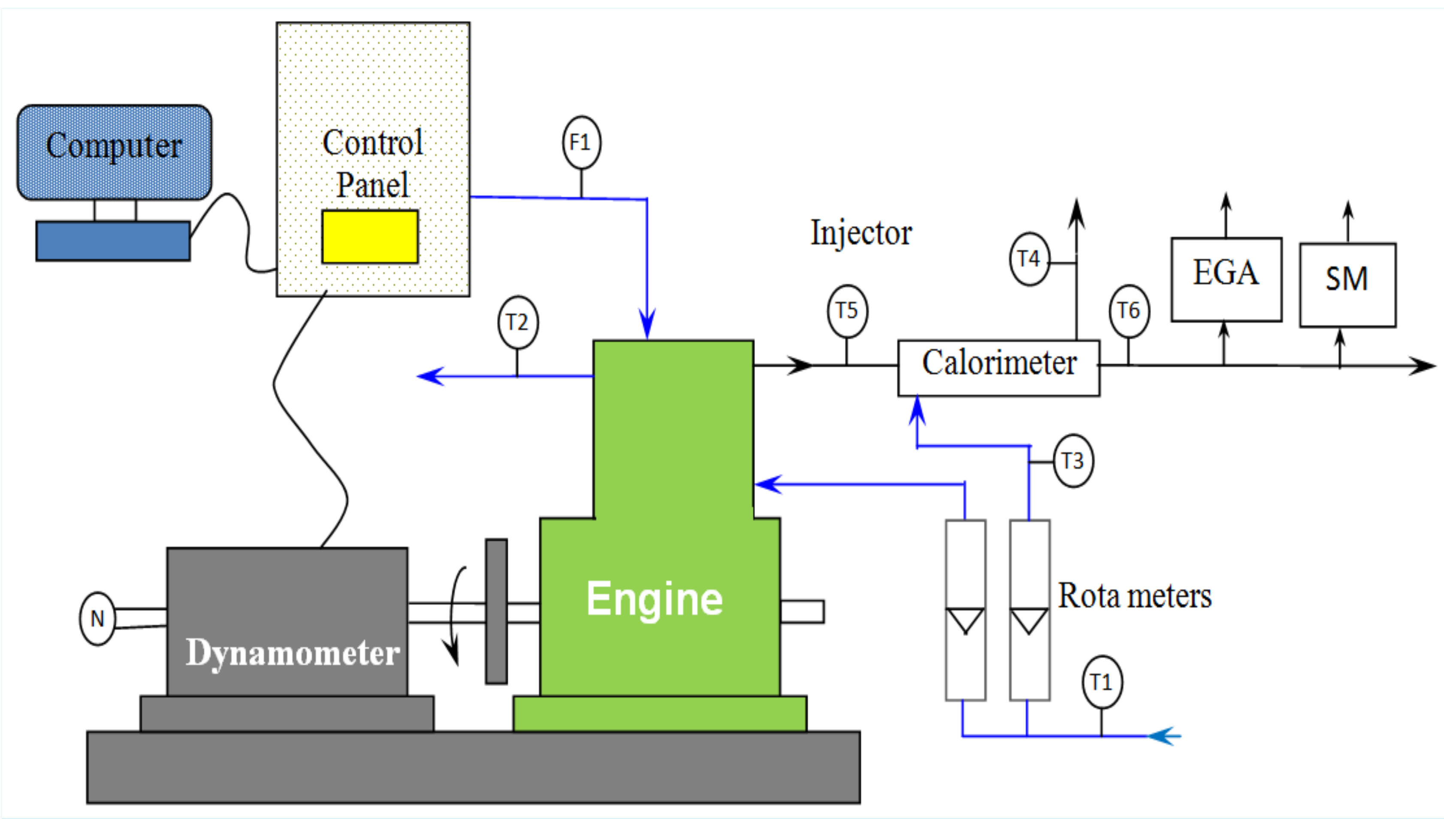
2.2. Experimentation Methodologies
2.3. Uncertainties Estimated
2.4. Design of Experiments and Experimentation
2.5. Response Surface Modelling and Assay
3. Results and Discussions
3.1. RSM Analysis
3.2. Performance Attributes
Brake Thermal Efficiency
3.3. Emission Attributes
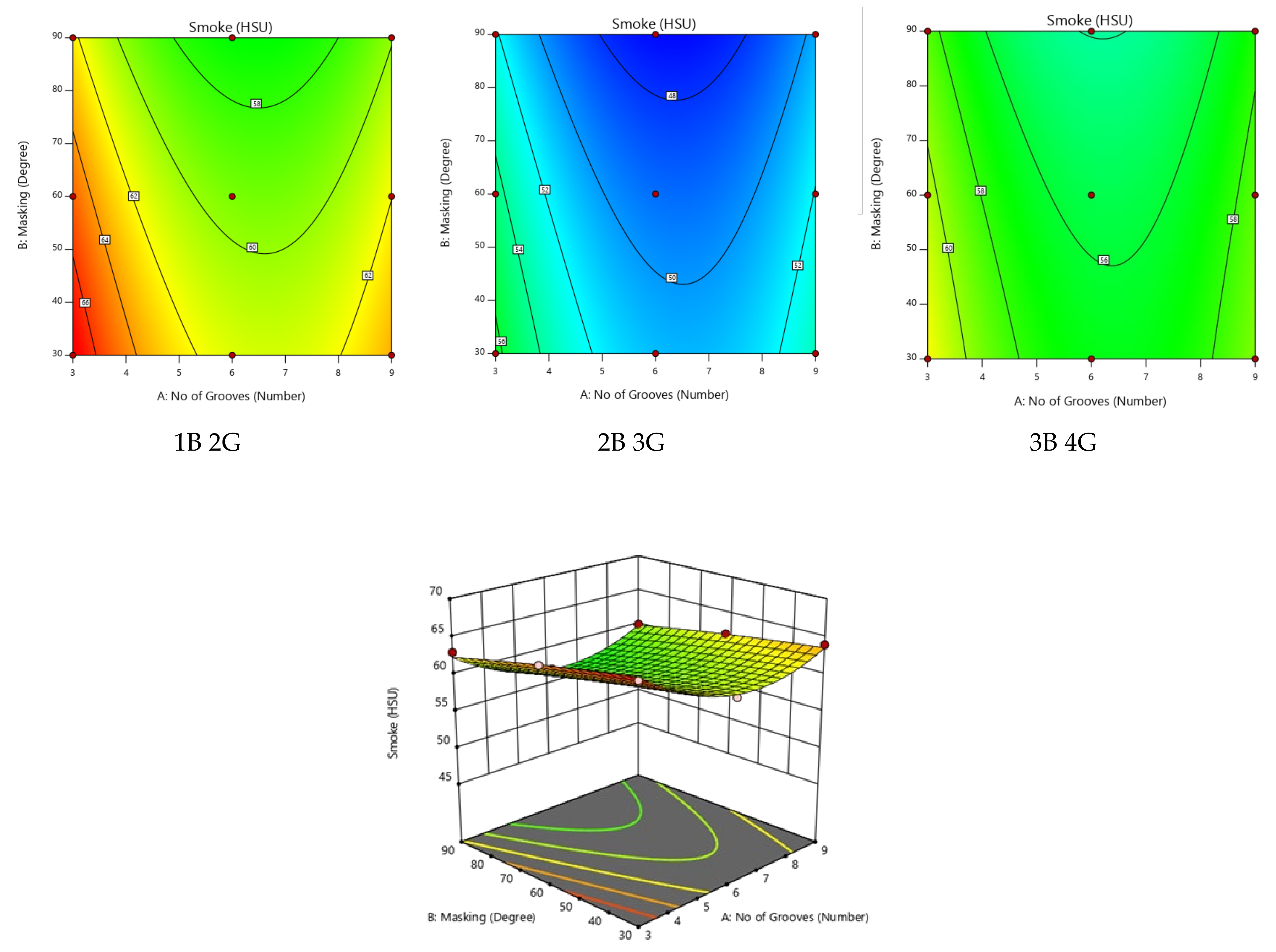
3.3.1. Smoke Emissions
3.3.2. HC Emissions
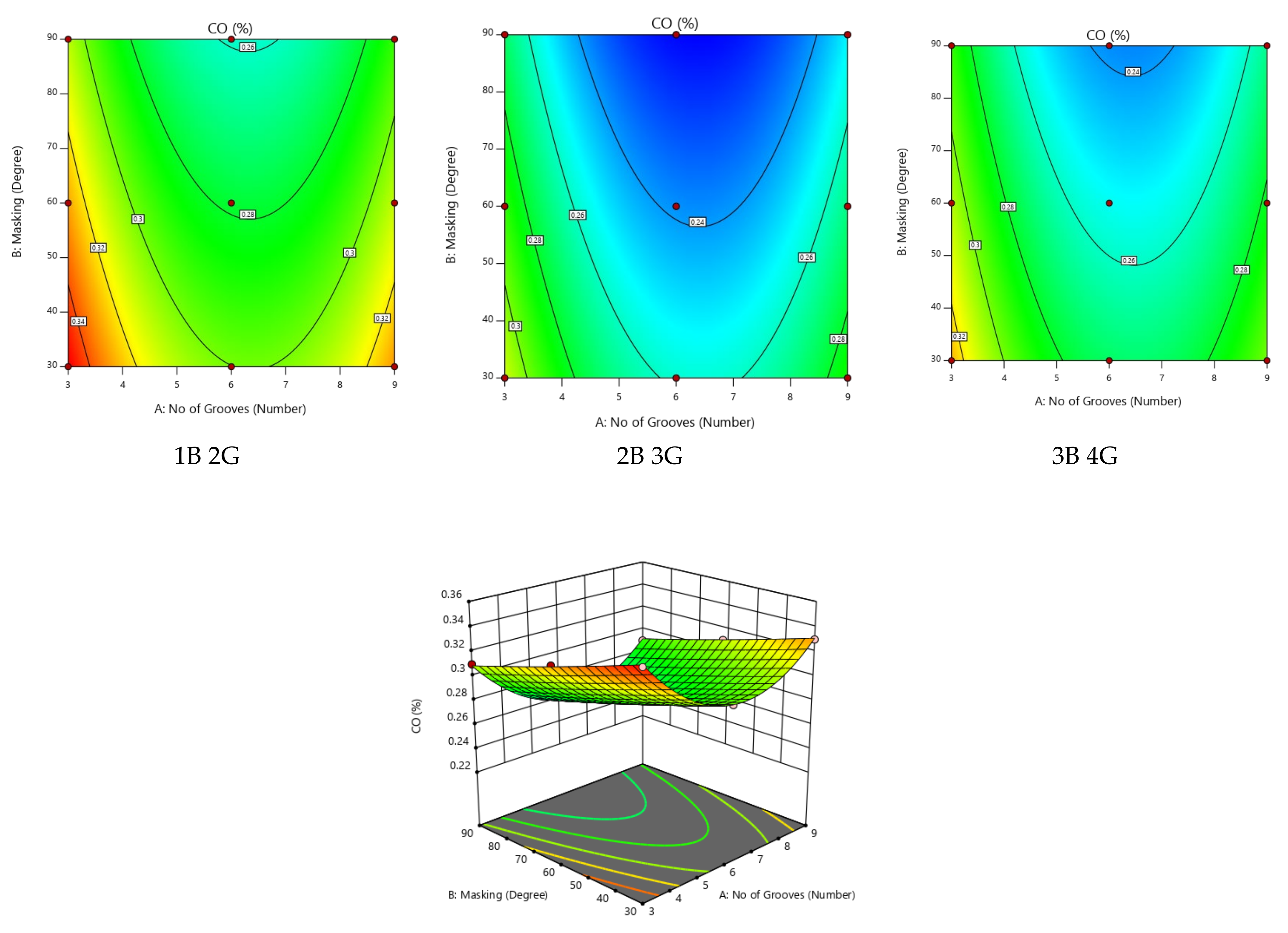
3.3.3. CO Emissions
3.3.4. NOx Emissions
3.4. Combustion Attributes
3.4.1. Peak Pressure (Pmax, PP)
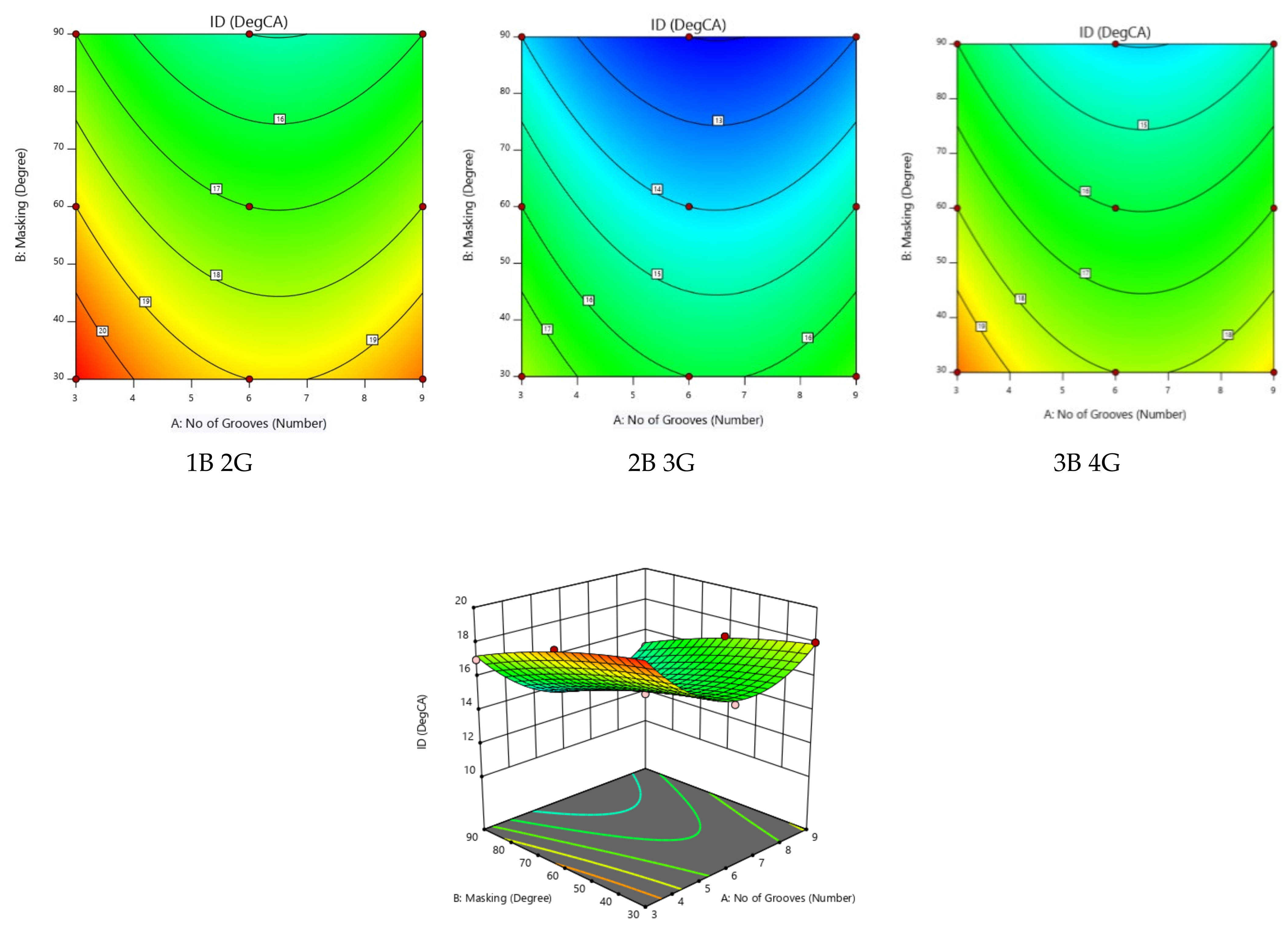
3.4.2. Ignition Delay (ID)
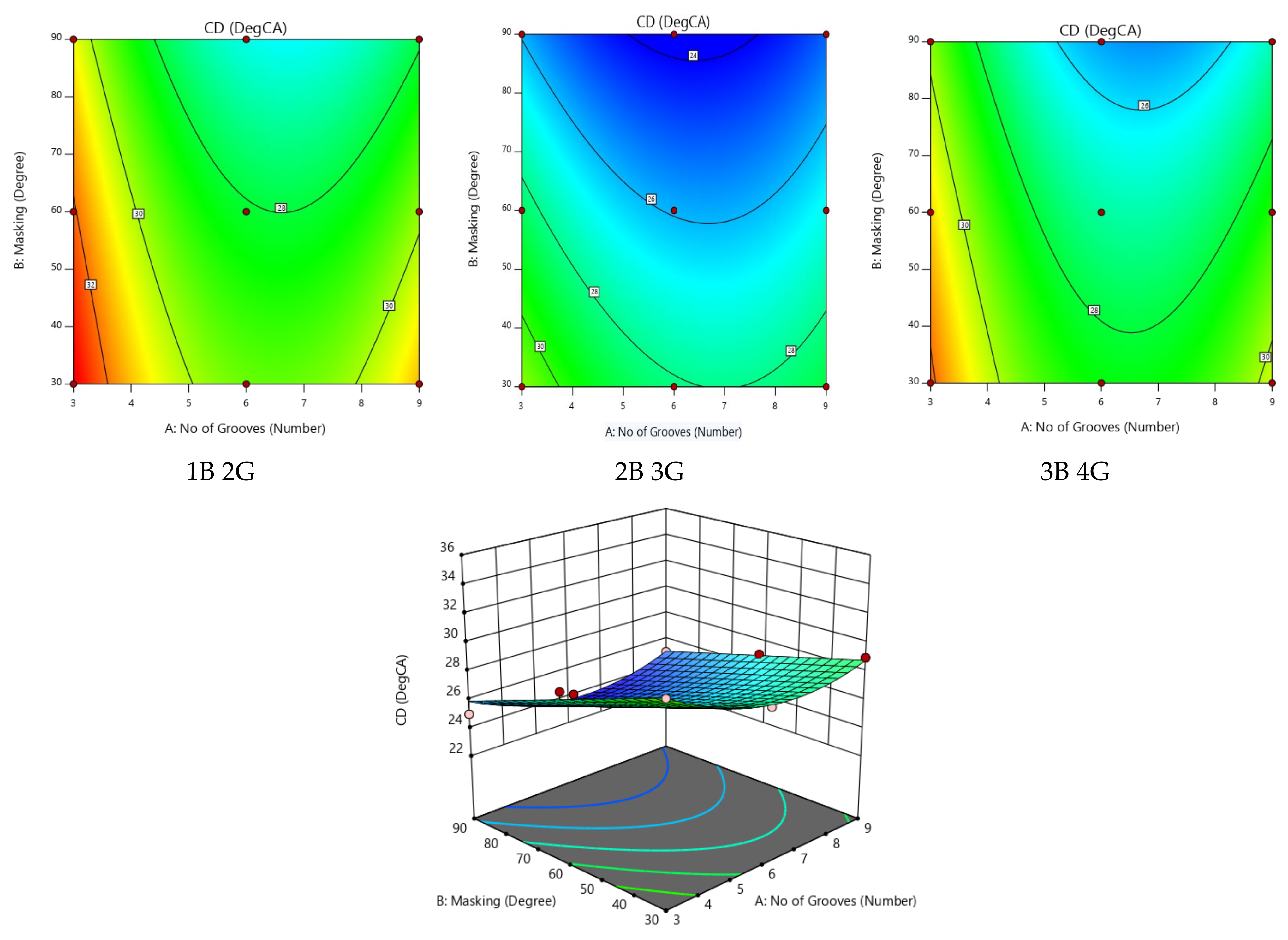
3.4.3. Combustion Duration (CD)
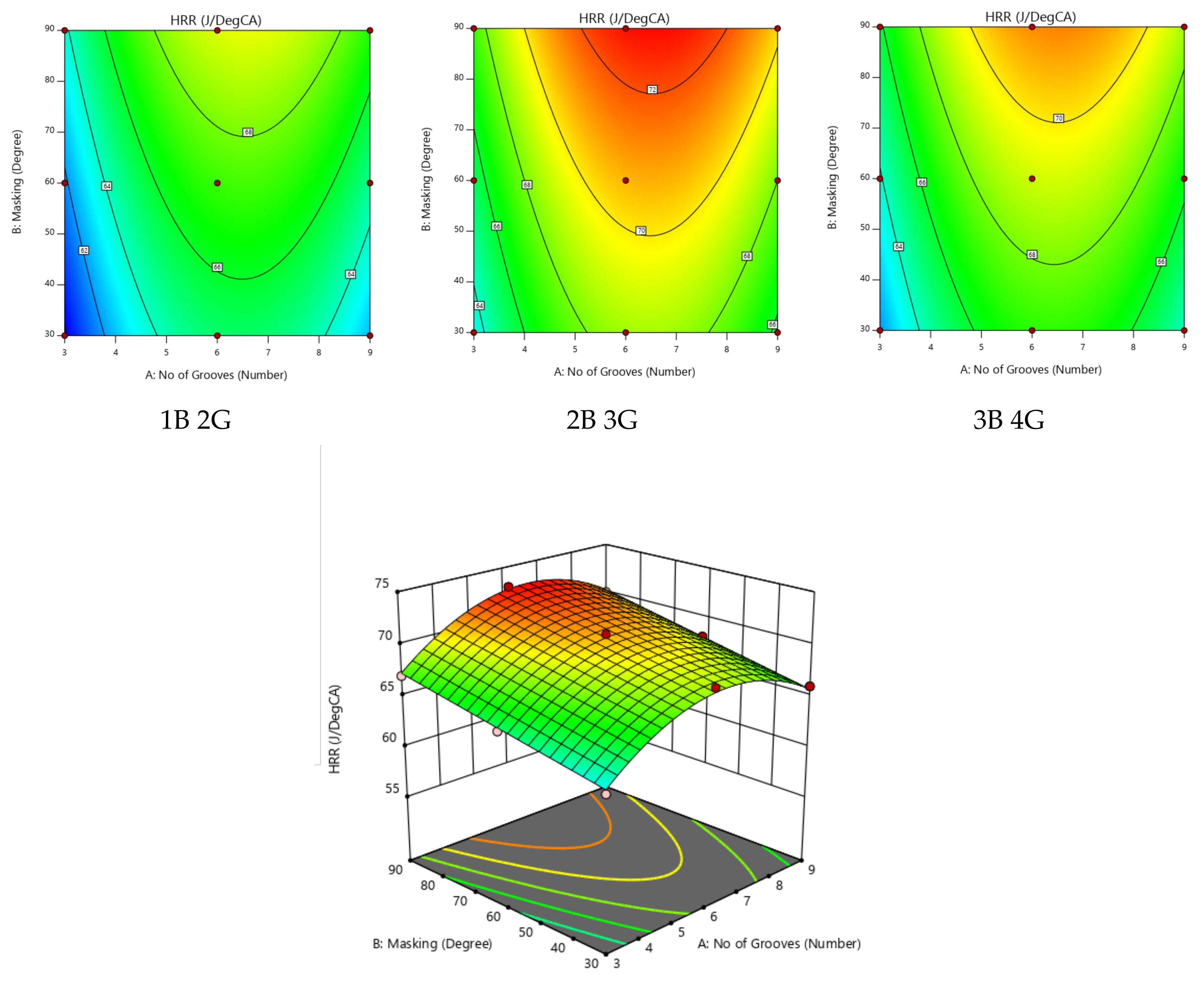
3.4.4. Heat Release Rate (HRR)
4. Validation of Test Results
4.1. Validation of Test Results for Optimized Conditions
4.2. Emission Norms Set by Worldwide Councils and Validation of Engine Test
4.3. Theoretical Calculations of Approximate Emission of Greenhouse Gases CO2 and NO2 Based on Diesel Consumption by Vehicles in g/km
5. Conclusions
- RSM is a powerful optimization tool for diesel engines fueled with HOME. Significant outcomes on the competence and emission attributes were assayed. A second-degree model was prosperously established to narrate the linkages among input parameter grooves on piston, inlet valve masking, and bridges and grooves on cylinder heads on output responses.
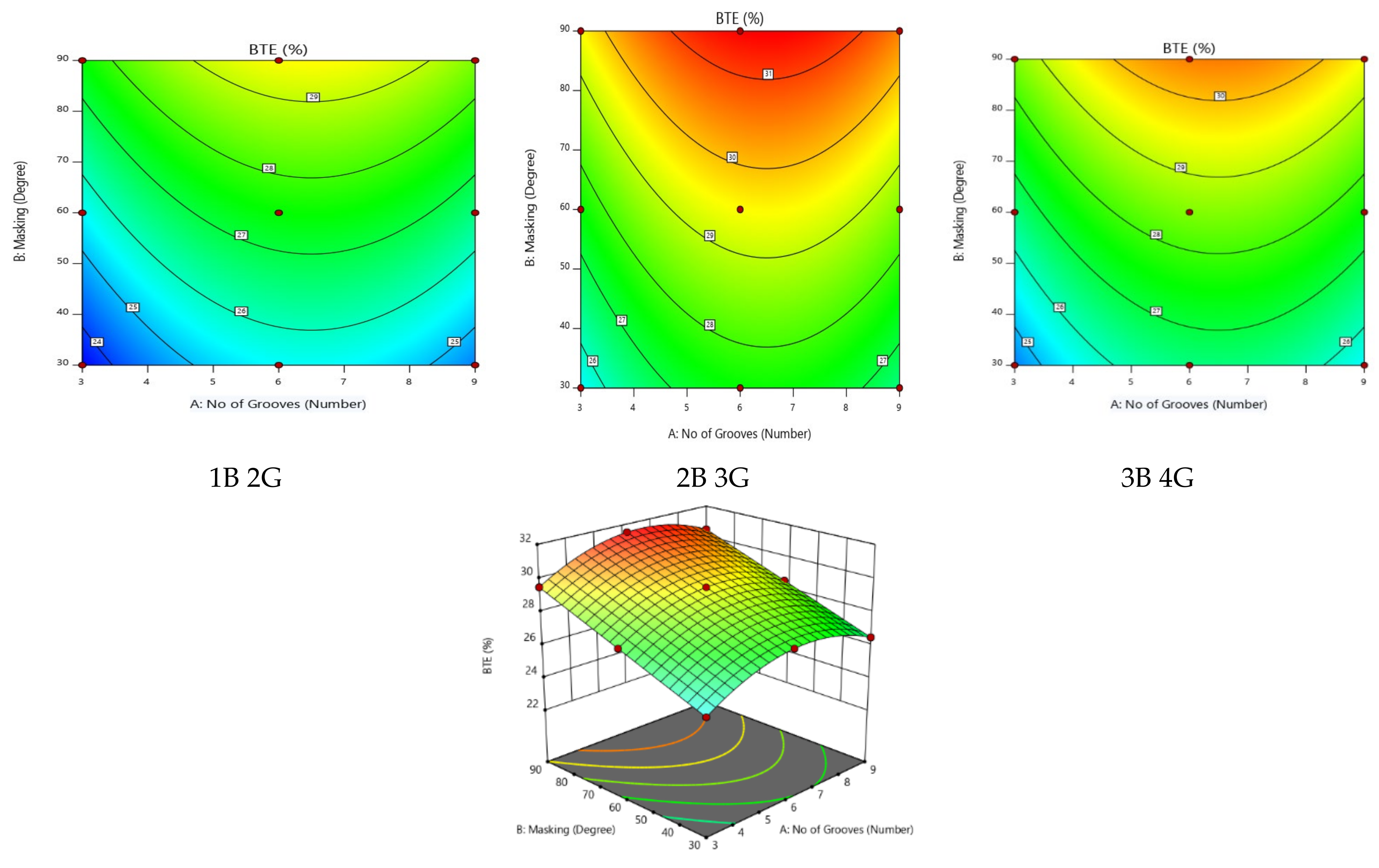
- Optimal input variables for maximizing performance and minimizing emissions, except NOx, are 2B 3G cylinder head, ‘IVM’ of 90°, and ‘NG’ of 6 grooves on the piston. RSM analysis of the experimental results optimizes outcome responses, as given below in Table 13.
- 3.
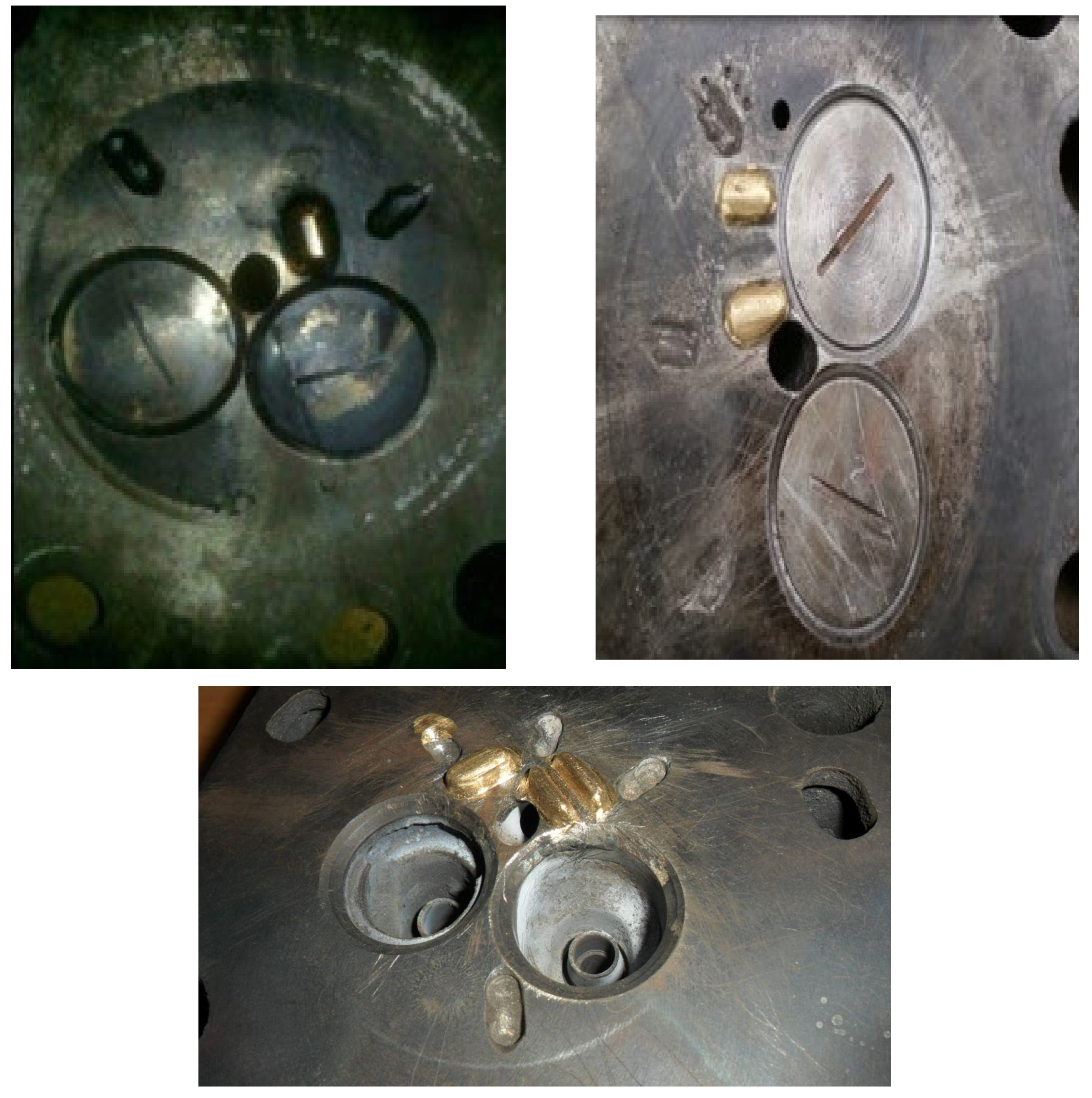
- Provision of bridges and grooves on the cylinder head proves to be very effective as they reduce emissions considerably. Additionally, a slight change in configuration of bridges and grooves can change flow directions and patterns and vary the way gases react, thus may reduce emissions further.
- 4.
- In RSM assay, BTE achieved for ‘NG’ of 6 and ‘IVM’ of 90° and 2B 3G cylinder head for HOME is 31.3679%, which is equal to BTE of diesel in a conventional engine. It is 3.3679% higher and 10.73% more compared to neat HOME operation in CI mode, which is 28%. In addition, BTE for the validity test was 29.94% less than the RSM value. Similarly, for the above combinations, smoke, HC, CO, and NOx were reduced by 28.5% (66 to 47.1852 HSU), 38.12% (65 to 40.2222 ppm), 36.93% (0.35 to 0.220741%), and by 15.26% (1009 to 855 ppm) compared to neat HOME operation in CI mode.
- 5.
- The assay of variances (ASOVA) revealed that this model could put forth the actual linkages among the outcomes and eloquent variables, with an acceptable overall or average determining coefficient R2 = 0.9862 of all responses, which directs that 98.62% of the adaptability for the responses could be described by the second-order polynomial predictors.
- 6.
- This optimized condition was validated by conducting an experiment and found similar results.
- 7.
- The other experimental design values of FFD and RSM values can also be considered in actual implementation in engine applications, keeping in view the response to be optimized.
- 8.
- Response surface assay-based quadratic predictors can be used with ease to create the linkages among the independent parameters and dependent characteristics.
- 9.
- The validation of predicted outputs shows that the quadratic predictors are accurate enough and in good agreement.
- 10.
- The effect of provision of bridges and grooves on cylinder heads proves to be an important parameter to improve competence and curtail emissions, but some other variables, such as injection pressure, injection timing, compression ratio, nozzle geometry, and speed, etc., should be tested and assayed alongside them.
- 11.
- According to the validation of test emission results as per CPCB India, the European Union, and the USA, the emissions are less than or very close to the norms and are in general around 10 g/kW-h, thus it can be stated that inlet valve masking (IVM) and number of piston grooves (NG) and cylinder head bridge-groove configuration (BGC) can be implemented for any diesel engines.
- 12.
- The major difference between the existing BS-IV and forthcoming BS-VI norms is the presence of diverse Sulphur compounds in the fuel. While the BS-IV fuel contains 50 parts per million (ppm) or mg/kg Sulphur, the BS-VI grade fuel only has 10 ppm or mg/kg Sulphur content. The different compounds of Sulphur form SO2, and 10% of SO3 formed combines with water to form H2SO4 aerosols, combining with soot and dust to form particulate matter. Additionally, the harmful NOx (nitrogen oxides) from diesel cars has to be brought down by nearly 70%. In the petrol cars, they can be reduced by 25%. However, when we discuss air pollution, particulate matter, such as PM 2.5 (particles smaller than 2.5 microns) and PM 10 (particles smaller than 10 microns), are the most harmful components, and the BS VI will bring down the cancer-causing particulate matter in diesel cars by a phenomenal 80%. As there is no Sulphur in BDF, there is no PM problem.
- 13.
- An IVM of 90°, a ‘NG’ on piston 6, and ‘BGC’ with 2B 3G model showed the highest NOx emissions of 855 ppm, which was 15.26% less contrasted with neat HOME utilized CI mode of working, which was 1009 and 900 ppm, respectively, with and without bridge-groove configuration. Lowered NOx emitted with other combinations may be linked to low combusting temperatures. It is to be noted that, for diesel engine simulation fueled with HOME, if we implement a combination of 1B 2G cylinder head, ‘IVM’ of 30° and ‘NG’ of 3 grooves on the piston optimizes a low NOx of 717.5 ppm (BTE decreases slightly from 31.3679% to 23.5215%). It is much less than that for neat HOME in a conventional engine, i.e., 1009 ppm. Hence, the percentage reduction of NOx is about 40.62%. This suffices, to some extent, emission standards BS 6 and Euro 6 (to be implemented from April 2020), which are planning to reduce NOx by a staggering 70% compared to BS 4 and Euro 5. For the time being, this large reduction has not been made possible by engine research only, as reported by İbrahim Aslan Reşitoğlu et al. [18]. Thus, by using further On Board Equipment (OBE) and Real Driving Emissions (RDE) on all vehicles, enabling real-time tracking of emissions, diesel vehicles will include a Diesel Particulate Filter (DPF) and Selective Catalytic Reduction (SCR) technologies. With these design changes, NOx may be decreased towards 70%. Additionally, by 2023, catalytic converters and misfire detectors are to be incorporated as per the (Automotive Research Association of India (ARAI), which is the leading automotive R&D organization of the country, set up by the Automotive Industry with the Government of India.
- 14.
- For 100% HOME biodiesel with a combination of inlet valve masking (IVM) of 90°, number of piston grooves (NG) of 6 grooves on piston crown, and cylinder head bridge-groove configuration (BGC) of 2B 3G, CO emissions are considerably reduced from 46.0 g/kW-h to 17.65 g/kW-h if we take the last readings for a full load of 5.2 kW, as given in Table 6. Thus, we can conclude that, for CO, BS VI norms cannot be satisfied only from engine research, as also reported by İbrahim Aslan Reşitoğlu et al. [18], and may be satisfied by on board equipment such as a DOC (diesel oxidation catalyst).
Author Contributions
Funding
Institutional Review Board Statement
Informed Consent Statement
Data Availability Statement
Acknowledgments
Conflicts of Interest
Nomenclature
| DOE | Designs of experiments |
| FFD | Full factorial designs |
| RSM | Response surface methodologies |
| ASTM | American Society for Testing and Materials |
| BTE | Brake thermal efficiency |
| BGC | Bridge-groove configuration |
| IVM | Inlet valve masking |
| CR | Compression ratio |
| SOC | Start of combustion |
| BDF | Biodiesel fuel |
| DICI | Direct injection compression ignition |
| IT | Injection timing |
| IOP | Injector opening pressure |
| EGR | Exhaust gas recirculation |
| TDC | Top dead center |
| bTDC | Before top dead center |
| a TDC | After top dead center |
| BSFC | Brake specific fuel consumption |
| ID | Ignition delay |
| CD | Combustion duration |
| NOx | Oxides of nitrogen |
| HC | Hydrocarbon |
| UBHC | Unburnt hydrocarbon |
| CO | Carbon monoxide |
| PM | Particulate matter |
| SI | Spark ignition |
| CA | Crank angle |
| PP | Peak pressure |
| HRR | Heat release rate |
| BTL | Burning time loss |
| EGT | Exhaust gas temperature |
References
- Agarwal, A.K.; Dhar, A.; Gupta, J.G.; Kim, W.I.; Choi, K.B.; Lee, C.S.; Park, S.W. Effect of fuel injection pressure and injection timing of Karanja biodiesel blends on fuel spray, engine performance, emissions and combustion characteristics. Energy Convers. Manag. 2015, 91, 302–314. [Google Scholar] [CrossRef]
- Goldenberg, J.; Coelhobn, S.T. Renewable energy—Traditional biomass vs. modern biomass. Energy Policy 2004, 32, 711–714. [Google Scholar] [CrossRef]
- Abuhabaya, A.; Fieldhouse, J.; Brow, D. The optimization of biodiesel production by using response surface methodology and its effect on compression ignition engine. Fuel Process. Technol. 2013, 113, 57–62. [Google Scholar] [CrossRef]
- Singh, Y.; Sharma, A.; Tiwari, S.; Singla, A. Optimization of diesel engine performance and emission parameters employing cassia tora methyl esters-response surface methodology approach. Energy 2018, 168, 909–918. [Google Scholar] [CrossRef]
- Ganapathy, T.; Murugesan, K.A.; Gakkhar, R.P. Performance optimization of Jatropha biodiesel engine model using Taguchi approach. Appl. Energy 2009, 86, 2476–2486. [Google Scholar] [CrossRef]
- Raheman, H.; Phadatare, A.G. Diesel engine emissions and performance from blends of Karanja methyl ester and diesel. Biomass Bioenergy 2004, 27, 393–397. [Google Scholar] [CrossRef]
- Hirkude, J.; Padalkar, A.; Shaikh, S.; Veigas, A. Effect of compression ratio on performance of CI engine fueled with biodiesel from waste fried oil using response surface methodology. Int. J. Energy Eng. 2013, 3, 227–233. [Google Scholar] [CrossRef]
- Rao, K.P.; Rao, B.V.A. Parametric optimization for performance and emissions of an IDI engine with Mahua biodiesel. Egypt. J. Pet. 2017, 26, 733–743. [Google Scholar]
- Berber, A. Mathematical model for fuel flow performance of diesel engine. Int. J. Automot. Eng. Technol. 2016, 5, 17–24. [Google Scholar] [CrossRef]
- Najafi, G. Diesel engine combustion characteristics using nano-particles in biodiesel-diesel blends. Fuel 2018, 212, 668–678. [Google Scholar] [CrossRef]
- Nayyar, A.; Sharma, D.; Soni, S.L.; Mathur, A. Characterization of n-butanol diesel blends on a small size variable compression ratio diesel engine: Modeling and experimental investigation. Energy Convers Manag. 2017, 150, 242–258. [Google Scholar] [CrossRef]
- Hosmath, R.S.; Banapurmath, N.R.; Khandal, S.V.; Gaitonde, V.N.; Basavarajappa, Y.H. Effect of compression ratio, CNG flow rate and injection timing on the performance of dual fuel engine operated on honge oil methyl ester (HOME) and compressed natural gas (CNG). Renew Energy 2016, 93, 579–590. [Google Scholar] [CrossRef]
- Khoobbakht, G.; Najafi, G.; Karimi, M.; Akram, A. Optimization of operating factors and blended levels of diesel, biodiesel and ethanol fuels to minimize exhaust emissions of diesel engine using response surface methodology. Appl. Therm. Eng. 2016, 99, 1006–1017. [Google Scholar] [CrossRef]
- Kumar, B.R.; Saravanan, S.; Rana, D.; Nagendra, A. Combined effect of injection timing and exhaust gas recirculation (EGR) on performance and emissions of a DI diesel engine fueled with next-generation advanced biofuel–diesel blends using response surface methodology. Energy Convers Manag. 2016, 123, 470–486. [Google Scholar] [CrossRef]
- Dhole, A.E.; Lata, D.B.; Yarasu, R.B. Effect of hydrogen and producer gas as secondary fuels on combustion parameters of a dual fuel diesel engine. Appl. Eng. 2016, 108, 764–773. [Google Scholar] [CrossRef]
- Pandal, A.; Payri, R.; García-Oliver, J.M.; Pastor, J.M. Optimization of spray break-up CFD simulations by combining Σ-Y Eulerian atomization model with response surface methodology under diesel engine-like conditions (ECN Spray A). Comput. Fluids 2017, 156, 9–20. [Google Scholar] [CrossRef] [Green Version]
- Pandian, M.; Sivapirakasam, S.P.; Udayakumar, M. Investigation on the effect of injection system parameters on performance and emission characteristics of a twin cylinder compression ignition direct injection engine fueled with pongamia biodiesel–diesel blend using response surface methodology. Appl. Energy 2011, 88, 2663–2676. [Google Scholar] [CrossRef]
- Reşitoğlu, İ.A.; Altinişik, K.; Keskin, A. The pollutant emissions from diesel-engine vehicles and exhaust aftertreatment systems. Clean Technol. Environ. Policy 2015, 17, 15–27. [Google Scholar] [CrossRef] [Green Version]
- Kaminaga, T.; Yamaguchi, K.; Ratnak, S.; Kusaka, J.; Youso, T.; Fujikawa, T.; Yamakawa, M. A study on combustion characteristics of a high compression ratio SI engine with high pressure gasoline injection. SAE Tech. Pap. 2019. [Google Scholar] [CrossRef]
- Ratnak, S.; Kusaka, J.; Daisho, Y.; Yoshimura, K.; Nakama, K. Experiments and simulations of a lean-boost spark ignition engine for thermal efficiency improvement. SAE Int. J. Engines 2016, 9, 379–396. [Google Scholar]
- Durakovic, B. Design of experiments application, concepts, examples: State of the art. Period. Eng. Nat. Sci. (PEN) 2017, 5, 421–439. [Google Scholar] [CrossRef]
- di Blasio, G.; Viscardi, M.; Beatrice, C. DoE method for operating parameter optimization of a dual-fuel bio ethanol/diesel light duty engine. J. Fuels 2015, 2015, 674705. [Google Scholar] [CrossRef] [Green Version]
- Win, Z.; Gakkhar, R.P.; Jain, S.C.; Bhattacharya, M. Parameter optimization of a diesel engine to reduce noise, fuel consumption, and exhaust emissions using response surface methodology. Proc. IMechE Part D J. Automob. Eng. 2005, 219, 1181–1192. [Google Scholar] [CrossRef]
- Myers, R.H.; Montgomery, D.C.; Anderson-Cook, C.M. Response Surface Methodology; John Wiley & Sons, Inc.: Hoboken, NJ, USA, 2009. [Google Scholar]
- Ganapathy, T.; Gakkhar, R.P.; Murugesan, K. Optimization of performance parameters of diesel engine with Jatropha biodiesel using response surface methodology. Int. J. Sustain. Energy 2011, 30, 76–90. [Google Scholar] [CrossRef]
- Adam, I.K.; Aziz, A.R.A.; Yusup, S. Determination of diesel engine performance fueled biodiesel (rubber seed/palm oil mixture) diesel blend. Int. J. Automot. Mech. Eng. IJAME 2015, 11, 2675–2685. [Google Scholar] [CrossRef]
- Yaliwal, V.S.; Nataraja, K.M.; Banapurmath, N.R.; Tewari, P.G. Honge oil methyl ester and producer gas-fueled dual-fuel engine operated with varying compression ratios. Int. J. Sustain. Eng. 2013, 7, 330–340. [Google Scholar] [CrossRef]


| Sl. NoN | Properties | Diesel | Honge Oil | HOME | ASTM Standards |
|---|---|---|---|---|---|
| 1 | Viscosity (c. St at 40 °C) | 4.59 | 56 | 5.6 | ASTMD445 |
| 2 | Flash point (°C) | 56 | 270 | 163 | ASTM D93 |
| 3 | Calorific Value (kJ/kg) | 45,000 | 35,800 | 36,100 | ASTM D5865 |
| 4 | Mass Density (kg/m3 at 15 °C) | 830 | 930 | 890 | ASTM D4052 |
| 5 | Cetane Number | 45–55 | 40 | 40–42 | ASTM D613 |
| 6 | Cloud Point (°C) | 15 | 13 | ASTM D2500 | |
| 7 | Pour Point (°C) | 1 | −2 to −5 | ||
| 8 | Carbon Residue (%) | 0.1 | 0.66 | ASTM D4530 | |
| 9 | Type of oil | Fossil fuel | Non edible | Non edible |
| Sl. No. | Parameters | Specifications |
|---|---|---|
| 1 | Engine type | TV1 (Kirloskar make) |
| 2 | Software interfaced | Engine soft |
| 3 | Injector opening pressure | 200 to 225 bar |
| 4 | Static injecting time | 23°bTDC |
| 5 | Governor type | Centrifugal type Mechanical |
| 6 | Number of cylinders | Single cylinder |
| 7 | Number of strokes | 4 strokes |
| 8 | Fuel oil | Diesel |
| 9 | Rated power | 5.2 kW at 1500 rpm |
| 10 | Cylinder diameter (Bore) | 0.0875 m |
| 11 | Stroke length | 0.11 m |
| 12 | Ratio of compression | 17.5: 1 |
| Variables | Notation and Units | Levels | ||
|---|---|---|---|---|
| Number of grooves on piston | G or A, Nr | 3 | 6 | 9 |
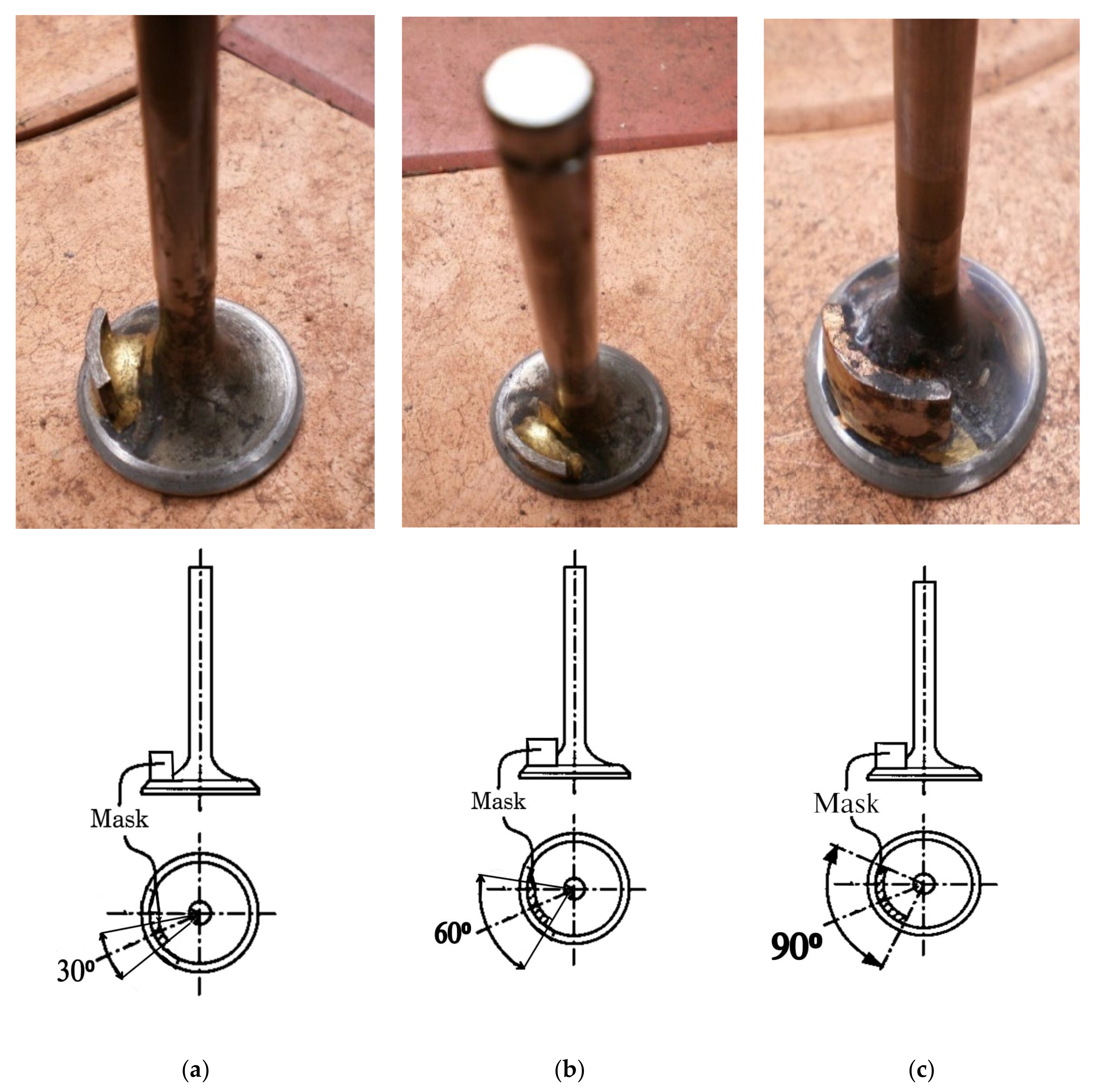
| Inlet valve masking | M or B, Degrees | 30 | 60 | 90 |
| Grooves and Bridges on Cylinder head | Br-Gr or C, Nr | 3 | 5 | 7 |
| Trial No. | Settings of Parameters | Responses Characteristics (80% Load) | ||||||||||
|---|---|---|---|---|---|---|---|---|---|---|---|---|
| No. of Grove | Masking | BR-GR | BTE | Smoke | HC | CO | NOx | Pmax | ID | CD | HRR | |
| (Degree) | (%) | (HSU) | (ppm) | (%) | (ppm) | (Bar) | (°CA) | (°CA) | (J/°CA) | |||
| 1 | 3 | 30 | 1B2G | 23.5 | 67 | 60 | 0.35 | 730 | 55 | 20 | 33 | 60 |
| 2 | 3 | 30 | 2B3G | 25.5 | 58 | 49 | 0.31 | 750 | 60 | 18 | 31 | 63 |
| 3 | 3 | 30 | 3B4G | 24.5 | 62 | 57 | 0.33 | 740 | 58 | 19 | 32 | 62 |
| 4 | 3 | 60 | 1B2G | 24.15 | 65 | 58 | 0.33 | 740 | 57 | 19 | 32 | 62 |
| 5 | 3 | 60 | 2B3G | 26.25 | 54 | 47 | 0.29 | 760 | 62 | 17 | 30 | 65 |
| 6 | 3 | 60 | 3B4G | 25.20 | 60 | 55 | 0.31 | 750 | 60 | 18 | 31 | 64 |
| 7 | 3 | 90 | 1B2G | 24.85 | 63 | 56 | 0.31 | 760 | 60 | 17 | 31 | 64 |
| 8 | 3 | 90 | 2B3G | 27.95 | 52 | 45 | 0.27 | 780 | 65 | 15 | 29 | 67 |
| 9 | 3 | 90 | 3B4G | 25.75 | 58 | 53 | 0.29 | 770 | 63 | 16 | 30 | 66 |
| 10 | 6 | 30 | 1B2G | 25.45 | 61 | 54 | 0.3 | 790 | 61 | 16 | 30 | 65 |
| 11 | 6 | 30 | 2B3G | 28.53 | 50 | 43 | 0.26 | 810 | 66 | 14 | 28 | 69 |
| 12 | 6 | 30 | 3B4G | 26.25 | 56 | 51 | 0.27 | 800 | 64 | 15 | 29 | 67 |
| 13 | 6 | 60 | 1B2G | 26.05 | 59 | 52 | 0.28 | 810 | 63 | 15 | 28 | 67 |
| 14 | 6 | 60 | 2B3G | 29.15 | 49 | 41 | 0.24 | 830 | 68 | 13 | 26 | 71 |
| 15 | 6 | 60 | 3B4G | 27.15 | 57 | 49 | 0.25 | 820 | 66 | 14 | 27 | 69 |
| 16 | 6 | 90 | 1B2G | 28.55 | 57 | 50 | 0.26 | 840 | 65 | 14 | 26 | 69 |
| 17 | 6 | 90 | 2B3G | 31.55 | 47 | 39 | 0.22 | 860 | 70 | 12 | 24 | 73 |
| 18 | 6 | 90 | 3B4G | 28.15 | 55 | 47 | 0.24 | 850 | 68 | 13 | 25 | 71 |
| 19 | 9 | 30 | 1B2G | 24.47 | 64 | 57 | 0.33 | 760 | 58 | 18 | 31 | 62 |
| 20 | 9 | 30 | 2B3G | 26.52 | 54 | 46 | 0.29 | 780 | 63 | 16 | 29 | 66 |
| 21 | 9 | 30 | 3B4G | 25.37 | 59 | 54 | 0.30 | 770 | 61 | 17 | 30 | 64 |
| 22 | 9 | 60 | 1B2G | 25.10 | 62 | 55 | 0.31 | 775 | 60 | 17 | 30 | 65 |
| 23 | 9 | 60 | 2B3G | 27.20 | 52 | 44 | 0.27 | 795 | 65 | 15 | 28 | 68 |
| 24 | 9 | 60 | 3B4G | 26.17 | 59 | 52 | 0.28 | 785 | 63 | 16 | 29 | 66 |
| 25 | 9 | 90 | 1B2G | 25.70 | 60 | 53 | 0.29 | 800 | 62 | 15 | 28 | 67 |
| 26 | 9 | 90 | 2B3G | 30.25 | 50 | 50 | 0.25 | 820 | 68 | 13 | 26 | 70 |
| 27 | 9 | 90 | 3B4G | 27.95 | 57 | 51 | 0.27 | 810 | 66 | 14 | 27 | 69 |
| Trial No. | Parameter Settings | Fitted Responses (80% Load) | ||||||||||
|---|---|---|---|---|---|---|---|---|---|---|---|---|
| No. of Grove | Masking | BR-GR | BTE | Smoke | HC | CO | NOx | Pmax | ID | CD | HRR | |
| (Degree) | (%) | (HSU) | (ppm) | (%) | (ppm) | (Bar) | (°CA) | (°CA) | (J/°CA) | |||
| 1 | 3 | 30 | 1B-2G | 23.5215 | 67.3796 | 60.2500 | 0.351574 | 717.5 | 55.1574 | 19.8889 | 33.1944 | 59.8611 |
| 2 | 3 | 30 | 2B-3G | 25.5694 | 56.4074 | 49.9722 | 0.311574 | 747.5 | 60.1019 | 17.8889 | 33.1944 | 63.3889 |
| 3 | 3 | 30 | 3B-4G | 24.3757 | 61.9907 | 57.0278 | 0.327130 | 737.5 | 57.9352 | 18.8889 | 33.1944 | 61.9167 |
| 4 | 3 | 60 | 1B-2G | 24.1174 | 65.0741 | 57.4167 | 0.329074 | 740.0 | 57.1574 | 18.8889 | 32.1111 | 61.8056 |
| 5 | 3 | 60 | 2B-3G | 26.2528 | 54.5185 | 47.2222 | 0.290741 | 760.0 | 62.1852 | 16.8889 | 30.1111 | 65.3333 |
| 6 | 3 | 60 | 3B-4G | 25.1465 | 60.5185 | 54.3611 | 0.307963 | 750.0 | 60.1019 | 17.8889 | 31.1111 | 63.8611 |
| 7 | 3 | 90 | 1B-2G | 24.7465 | 62.3241 | 55.5833 | 0.308796 | 762.5 | 59.7130 | 17.2222 | 30.6944 | 63.7500 |
| 8 | 3 | 90 | 2B-3G | 27.9694 | 52.1852 | 45.4722 | 0.272130 | 782.5 | 64.8241 | 15.2222 | 28.6944 | 67.2778 |
| 9 | 3 | 90 | 3B-4G | 25.9507 | 58.6019 | 52.6944 | 0.291019 | 772.5 | 62.8241 | 16.2222 | 29.6944 | 65.8056 |
| 10 | 6 | 30 | 1B-2G | 25.4458 | 61.3796 | 53.4167 | 0.300185 | 795.0 | 60.8241 | 16.2222 | 29.4444 | 65.1111 |
| 11 | 6 | 30 | 2B-3G | 28.3167 | 50.7407 | 43.2222 | 0.258519 | 815.0 | 65.8519 | 14.2222 | 27.4444 | 68.5556 |
| 12 | 6 | 30 | 3B-4G | 26.3458 | 56.6574 | 50.3611 | 0.272407 | 805.0 | 63.7685 | 15.2222 | 28.4444 | 67.0000 |
| 13 | 6 | 60 | 1B-2G | 26.0667 | 59.4074 | 51.3333 | 0.278519 | 810.0 | 62.7407 | 15.2222 | 28.1111 | 67.2222 |
| 14 | 6 | 60 | 2B-3G | 28.8250 | 49.1852 | 41.2222 | 0.238519 | 830.0 | 67.8519 | 13.2222 | 26.1111 | 70.6667 |
| 15 | 6 | 60 | 3B-4G | 27.1417 | 55.5185 | 48.4444 | 0.254074 | 820.0 | 65.8519 | 14.2222 | 27.1111 | 69.1111 |
| 16 | 6 | 90 | 1B-2G | 28.7208 | 56.9907 | 50.2500 | 0.259074 | 835.0 | 65.2130 | 13.5556 | 26.4444 | 69.3333 |
| 17 | 6 | 90 | 2B-3G | 31.3679 | 47.1852 | 40.2222 | 0.220741 | 855.0 | 71.4074 | 11.5556 | 24.4444 | 72.7778 |
| 18 | 6 | 90 | 3B-4G | 27.9708 | 53.9352 | 47.5278 | 0.237963 | 845.0 | 68.4907 | 12.5556 | 25.4444 | 71.2222 |
| 19 | 9 | 30 | 1B-2G | 24.4118 | 63.6019 | 56.5833 | 0.331019 | 757.5 | 58.0463 | 17.8889 | 31.3611 | 62.3611 |
| 20 | 9 | 30 | 2B-3G | 26.5056 | 53.2963 | 46.4722 | 0.287685 | 777.5 | 63.1574 | 15.8889 | 29.3611 | 65.7222 |
| 21 | 9 | 30 | 3B-4G | 25.3576 | 59.5463 | 53.6944 | 0.299907 | 767.5 | 61.1574 | 16.8889 | 30.3611 | 64.0833 |
| 22 | 9 | 60 | 1B-2G | 25.0576 | 61.9630 | 55.2500 | 0.310185 | 775.0 | 59.8796 | 16.8889 | 29.7778 | 64.6389 |
| 23 | 9 | 60 | 2B-3G | 27.2389 | 52.0741 | 45.2222 | 0.268519 | 795.0 | 65.0741 | 14.8889 | 27.7778 | 68.0000 |
| 24 | 9 | 60 | 3B-4G | 26.1785 | 58.7407 | 52.5278 | 0.282407 | 785.0 | 63.1574 | 15.8889 | 28.7778 | 66.3611 |
| 25 | 9 | 90 | 1B-2G | 25.7368 | 59.8796 | 54.9167 | 0.291574 | 802.5 | 62.2685 | 15.2222 | 27.8611 | 66.9167 |
| 26 | 9 | 90 | 2B-3G | 30.1056 | 50.4074 | 44.9722 | 0.251574 | 822.5 | 67.5463 | 13.2222 | 25.8611 | 70.2778 |
| 27 | 9 | 90 | 3B-4G | 27.0326 | 57.4907 | 52.3611 | 0.267130 | 812.5 | 65.7130 | 14 | 26.8611 | 68.6389 |
| Response | BTE | Smoke | HC | CO | NOx | Pmax | ID | CD | HRR |
|---|---|---|---|---|---|---|---|---|---|
| Regression | 0.001 | 0.002 | 0.002 | 0.001 | 0.005 | 0.000 | 0.000 | 0.000 | 0.001 |
| Linear | 0.000 | 0.002 | 0.000 | 0.000 | 0.000 | 0.003 | 0.000 | 0.001 | 0.000 |
| Number of Grooves | 0.000 | 0.000 | 0.005 | 0.000 | 0.006 | 0.001 | 0.000 | 0.000 | 0.000 |
| Masking | 0.077 | 0.094 | 0.086 | 0.000 | 0.477 | 0.052 | 1.000 | 0.657 | 0.010 |
| Grooves | 0.002 | 0.002 | 0.003 | 0.000 | 0.003 | 0.001 | 0.000 | 0.002 | 0.000 |
| Square | 0.006 | 0.055 | 0.005 | 0.000 | 0.002 | 0.002 | 0.001 | 0.000 | 0.000 |
| Number of Grooves ∗ No of Grooves | 0.010 | 0.020 | 0.000 | 0.030 | 0.003 | 0.057 | 0.002 | 0.000 | 0.045 |
| Masking ∗ Masking | 0.714 | 0.492 | 0.429 | 0.248 | 0.004 | 0.029 | 0.010 | 0.310 | 1.000 |
| Grooves ∗ Grooves | 0.003 | 0.040 | 0.003 | 0.000 | 0.010 | 0.022 | 0.000 | 0.000 | 0.010 |
| Interaction | 0.063 | 0.083 | 0.413 | 0.013 | 0.170 | 0.406 | 1.000 | 0.216 | 0.304 |
| Number of Grooves ∗ Masking | 0.440 | 0.155 | 0.104 | 0.222 | 0.029 | 0.325 | 1.000 | 0.040 | 0.094 |
| Number of Grooves ∗ Grooves | 0.479 | 0.155 | 0.851 | 0.021 | 1.000 | 0.325 | 1.000 | 1.000 | 0.388 |
| Masking ∗ Grooves | 0.013 | 0.080 | 0.851 | 0.021 | 1.000 | 0.325 | 1.000 | 1.000 | 1.000 |
| Response | BTE | Smoke | HC | CO | NOx | Pmax | ID | CD | HRR |
|---|---|---|---|---|---|---|---|---|---|
| Mean | 26.5139 | 59.7005 | 50.6666 | 0.27495 | 788.3333 | 62.8889 | 15.7777 | 29.1851 | 66.3333 |
| Range | 7.8464 | 20.1944 | 20.0278 | 0.130833 | 137.5 | 16.25 | 8.3333 | 8.75 | 12.9167 |
| Variance | 3.5902 | 33.026 | 26.3673 | 0.0009456 | 1158.333 | 13.8556 | 4.1234 | 5.6855 | 9.7109 |
| Standard Deviation | 1.894 | 5.7468 | 5.1349 | 0.03075 | 34.0343 | 3.7223 | 2.0306 | 2.3844 | 3.1162 |
| Model Degree | Linear, Quadratic and Interactive | Linear and Quadratic | Linear and Quadratic | Linear and Quadratic | Linear and Quadratic | Linear and Quadratic | Linear and Quadratic | Linear Quadratic and Interactive | Linear and Quadratic |
| R2 | 99.58 | 98.50 | 94.78 | 99.67 | 99.29 | 99.62 | 98.82 | 98.08 | 99.32 |
| PRESS | 0.598056 | 25.1137 | 99.2654 | 0.000236424 | 587.972 | 3.62095 | 3.33283 | 6.71292 | 4.65460 |
| Predicted R2 | 98.76 | 96.30 | 86.66 | 99.10 | 98.13 | 98.99 | 97.04 | 95.02 | 98.24 |
| Adjusted R2 | 99.35 | 97.70 | 92.01 | 99.49 | 98.91 | 99.41 | 98.19 | 97.07 | 98.95 |
| Sum of Squares | Degrees of Freedom | Mean Square | F-Ratio | R2 | ||||
|---|---|---|---|---|---|---|---|---|
| Regression, SST | Residual | Regression | Residual | Regression | Residual | |||
| BTE | 48.0350 | 0.2042 | 9 | 17 | 5.3372 | 0.0120 | 444.37 | 0.9958 |
| Smoke | 669.417 | 10.213 | 9 | 17 | 74.38 | 0.601 | 123.81 | 0.9850 |
| HC | 705.139 | 38.861 | 9 | 17 | 78.349 | 2.286 | 34.27 | 0.9478 |
| CO | 0.026186 | 0.000088 | 9 | 17 | 0.002910 | 0.000005 | 562.31 | 0.9967 |
| NOx | 31275.0 | 225.0 | 9 | 17 | 3475.0 | 13.2 | 262.56 | 0.9929 |
| Pmax | 358.028 | 1.38 | 9 | 17 | 39.781 | 0.081 | 490.19 | 0.9962 |
| ID | 111.333 | 1.333 | 9 | 17 | 12.3704 | 0.0784 | 157.72 | 0.9882 |
| CD | 132.083 | 2.583 | 9 | 17 | 14.6759 | 0.1520 | 98.58 | 0.9808 |
| HRR | 262.194 | 1.806 | 9 | 17 | 29.1327 | 0.1062 | 274.3 | 0.9932 |
| Response | BTE % | Smoke HSU | HC ppm | CO % | NOx ppm | Pmax Bar | ID (°CA) | CD (°CA) | HRR (J/°CA) |
|---|---|---|---|---|---|---|---|---|---|
| Predicted | 31.3679 | 47.1852 | 40.2222 | 0.220741 | 855.0 | 71.4074 | 11.5556 | 24.4444 | 72.7778 |
| Actual | 29.94 | 55 | 46 | 0.24 | 820 | 66 | 14 | 32 | 67 |
| Error% | −4.5521 | 16.56 | 14.36 | 8.72 | −4.09 | −7.572 | 21.15 | 30.91 | −7.938 |
| S.No | N (rpm) | Time for 20 cc Fuel Consumption (s) | Air Consumption (m3/h) | EGT (°C) | NOx (ppm) | HC (ppm) | CO (%vol)/ppm |
|---|---|---|---|---|---|---|---|
| 1 | 1500 | 84.99 | 28.1 | 170 | 220 | 20 | 0.05/500 |
| 2 | 1500 | 69.78 | 30.46 | 216 | 380 | 25 | 0.08/800 |
| 3 | 1500 | 53.53 | 30.89 | 250 | 520 | 30 | 0.10/1000 |
| 4 | 1500 | 34.50 | 28.57 | 325 | 710 | 45 | 0.15/1500 |
| 5 | 1500 | 31.63 | 29.29 | 340 | 850 | 70 | 0.28/2800 |
| Brake Power (kW) | Mass of Fuel (kg/s) | BSFC (g/kWh) | Mass of Air (kg/s) | A/F Ratio | BMEP (Bar) | BTE (%) | Volumetric Efficiency (%) | NOx (g/kWh) | CO (g/kWh) | HC (g/kWh) |
|---|---|---|---|---|---|---|---|---|---|---|
| 1.04 | 0.00019531 | 417.63 | 0.007982 | 40.86 | 1.27 | 16.98 | 88.61 | 6.641 | 15.16 | 1.78 |
| 2.08 | 0.00023789 | 287.93 | 0.008293 | 34.86 | 2.54 | 24.22 | 86.89 | 10.81 | 12.65 | 2.22 |
| 3.12 | 0.00031010 | 236.33 | 0.008411 | 27.12 | 3.81 | 27.87 | 86.67 | 16.17 | 10.78 | 2.67 |
| 4.16 | 0.00048110 | 226.48 | 0.007778 | 16.17 | 5.08 | 29.94 | 84.52 | 22.08 | 11.48 | 4.00 |
| 5.20 | 0.00052475 | 211.53 | 0.007974 | 15.19 | 6.35 | 27.45 | 80.65 | 26.43 | 17.65 | 6.23 |
| S.No | Brake Power (kW) | For Diesel | For HOME | For Validation Test | |||
|---|---|---|---|---|---|---|---|
| CO (%vol)/ppm | CO (g/kWh) | CO (%vol)/ppm | CO (g/kWh) | CO (%vol)/ppm | CO (g/kWh) | ||
| 1 | 1.04 | 0.03/300 | 9.906 | 0.08/800 | 24.25 | 0.05/500 | 15.16 |
| 2 | 2.08 | 0.04/400 | 6.320 | 0.09/900 | 14.23 | 0.08/800 | 12.65 |
| 3 | 3.12 | 0.06/600 | 6.46 | 0.12/1200 | 12.93 | 0.10/1000 | 10.78 |
| 4 | 4.16 | 0.1/1000 | 10.78 | 0.25/2500 | 19.13 | 0.15/1500 | 11.48 |
| 5 | 5.20 | 0.35/3500 | 22.06 | 0.73/7300 | 46.01 | 0.28/2800 | 17.65 |
| Trial No. | Parameter Settings | Fitted Responses (80% Load) | ||||||||||
|---|---|---|---|---|---|---|---|---|---|---|---|---|
| No. of Grove | Masking | BR-GR | BTE | Smoke | HC | CO | NOx | Pmax | ID °CA | CD °CA | HR R | |
| (Degree) | (%) | (HSU) | (ppm) | (%) | (ppm) | (Bar) | J/°CA | |||||
| 1 | 3 | 30 | 1B-2G | 23.5215 | 67.3796 | 60.2500 | 0.351574 | 717.5 | 55.1574 | 19.8889 | 33.1944 | 59.8611 |
| 17 | 6 | 90 | 2B-3G | 31.3679 | 47.1852 | 40.2222 | 0.220741 | 855.0 | 71.4074 | 11.5556 | 24.4444 | 72.7778 |
Publisher’s Note: MDPI stays neutral with regard to jurisdictional claims in published maps and institutional affiliations. |
© 2021 by the authors. Licensee MDPI, Basel, Switzerland. This article is an open access article distributed under the terms and conditions of the Creative Commons Attribution (CC BY) license (https://creativecommons.org/licenses/by/4.0/).
Share and Cite
Indudhar, M.R.; Banapurmath, N.R.; Rajulu, K.G.; Patil, A.Y.; Javed, S.; Khan, T.M.Y. Optimization of Piston Grooves, Bridges on Cylinder Head, and Inlet Valve Masking of Home-Fueled Diesel Engine by Response Surface Methodology. Sustainability 2021, 13, 11411. https://doi.org/10.3390/su132011411
Indudhar MR, Banapurmath NR, Rajulu KG, Patil AY, Javed S, Khan TMY. Optimization of Piston Grooves, Bridges on Cylinder Head, and Inlet Valve Masking of Home-Fueled Diesel Engine by Response Surface Methodology. Sustainability. 2021; 13(20):11411. https://doi.org/10.3390/su132011411
Chicago/Turabian StyleIndudhar, Mathad R., Nagaraj R. Banapurmath, K. Govinda Rajulu, Arun Y. Patil, Syed Javed, and T. M. Yunus Khan. 2021. "Optimization of Piston Grooves, Bridges on Cylinder Head, and Inlet Valve Masking of Home-Fueled Diesel Engine by Response Surface Methodology" Sustainability 13, no. 20: 11411. https://doi.org/10.3390/su132011411