Article

Estimation of Current and Future Suitable Areas for Tapirus pinchaque in Ecuador

by
Carlos Mestanza-Ramón
1,2,*,
Robinson J. Herrera Feijoo
3,*,
Cristhian Chicaiza-Ortiz
3,4,5,6,7,
Isabel Domínguez Gaibor
8,9 and
Rubén G. Mateo
10,11
1
Instituto Superior Tecnológico Universitario Oriente, La Joya de los Sachas, Orellana 20101, Ecuador
2
Research Group YASUNI-SDC, Escuela Superior Politécnica de Chimborazo, Sede Orellana, El Coca EC 220001, Ecuador
3
Facultad Ciencias de la Vida, Universidad Estatal Amazónica, Puyo EC160150, Ecuador
4
China-UK Low Carbon College, Shanghai Jiao Tong University, Shanghai 200240, China
5
Facultad de Ciencias de la Vida, Universidad Regional Amazónica IKIAM, Tena, Napo 150150, Ecuador
6
Programa en Cambio Climático, Sustentabilidad y Desarrollo, Área de Ambiente y Sustentabilidad, Universidad Andina Simón Bolívar, Quito 170102, Ecuador
7
Grupo Internacional de Fomento a la Excelencia, Quito 170102, Ecuador
8
Facultad de Silvicultura e Ingeniería Forestal, Universidad Transilvania de Brasov, 500036 Brasov, Romania
9
Facultad de Ciencias, Escuela Superior Politécnica de Chimborazo, Sede Orellana EC140101, Ecuador
10
Departamento de Biología (Botánica), Universidad Autónoma de Madrid, C/Darwin 2, 28049 Madrid, Spain
11
Centro de Investigación en Biodiversidad y Cambio Global (CIBC-UAM), Universidad Autónoma de Madrid, 28049 Madrid, Spain
*
Authors to whom correspondence should be addressed.
Sustainability 2021, 13(20), 11486; https://doi.org/10.3390/su132011486
Submission received: 25 August 2021 / Revised: 15 October 2021 / Accepted: 15 October 2021 / Published: 18 October 2021
(This article belongs to the Special Issue Mammal Status: Diversity, Abundance and Dynamics)

Abstract

:
At present, climate change is a direct threat to biodiversity and its effects are evidenced by an increasingly accelerated loss of biodiversity. This study identified the main threats presently facing the Tapirus pinchaque species in Ecuador, generated predictive models regarding its distribution, and analyzed the protected areas as a conservation tool. The methodology was based on a literature review and the application of binary predictive models to achieve these objectives. The main results indicate that the T. pinchaque is seriously threatened, mainly by changes in land use. In addition, three models were selected that show current and future suitable areas for the conservation of the species. Its current distribution amounts to 67,805 km2, 33% (22,872 km2) of which is located in 31 of the 61 protected areas. Finally, it is important to take timely actions focused on biodiversity conservation, considering the importance of balance in ecosystems to the humans dependent thereof, and the results regarding the changes in the current and future distribution areas of the mountain tapir are a great contribution to be used as a management tool for its conservation.

1. Introduction

Biodiversity is a multidimensional, interdependent, and complex network, which as a whole and in a functional way provides ecosystem goods to humans [1,2]. All these types of life generate a balance between the different ecosystems, allowing a correct functionality, contributing to the generation of services that are used by human beings [3,4]. At present, the loss of biodiversity is one of the great challenges facing the planet. Although the reasons are varied, human activity is one of the main factors influencing the extinction of species [5]. Biodiversity is not only important because of its natural value as part of life support systems, but also because it has a very large economic potential which has not yet been valued in global planning [6,7]. Knowing the causes of biodiversity loss is essential to begin to reverse the situation and ensure the future of life on Earth [8,9].
Globally, climate change, invasive species, deforestation, overexploitation of natural resources, and pollution, among other human activities, are causing the most serious biodiversity crisis since the extinction of the dinosaurs 65 million years ago [10,11]. This is no different in Ecuador, where, along with cattle ranching, oil extraction and mining are currently the greatest threats to biodiversity [12,13]. The magnitude of the problem is such that the Intergovernmental Panel on Climate Change indicates that, of the species studied, around 50% have already been affected by climate change. The effects of this phenomenon on biodiversity can be explained by the fact that the particular environmental conditions for each species are significantly disrupted, preventing them from adapting [14,15]. The effects of climate change on life can be observed at different levels, in interactions with other species, in the extent of their geographic distribution, and even in the ecosystems themselves [16]. At this level, responses to changes in environmental variables begin to be noticeable [9,17]. Their effects have been documented in almost all taxonomic groups, including plants, insects, amphibians, birds, and mammals [12,18]. Importantly, not all species have the ability to move to new locations to avoid the effects of climate change. If they cannot adapt locally to the new conditions, they could become extinct in the medium to long term [19,20].
Throughout South America run the Andes, the most extensive mountain range on Earth, with a length of more than 7000 km [21]. This mountain range has 31 million hectares of forest, which is crucial for the region and the world. It is home to more than 87 million people, and contains various exceptional ecosystems, including paramos, cloud forests, and wetlands [22,23]. An essential part of this mountain range are the montane forests. Two of the most important hot spots on the planet, the tropical Andes and Tumbes Choco-Magdalena, are located in this area. Approximately 25% to 27% of the planet’s plant diversity is located in this zone. The Andean zone ecosystems exhibit privileged and unique characteristics that have facilitated speciation and biological evolution [24]. On the other hand, the Andes in the lower zones, called the tropical zones, are one of the most biodiverse regions on Earth [22]. In addition, the Andes provide elemental ecosystem services, such as water supply or carbon sequestration, to the more than 50 million people living in or near the most extended mountain range on the planet. More than 60% of the water available in the Amazon basin originates in this mountain range [25,26,27]. Ecuador is the country with the highest number of species per square kilometer.
The Andean tapir (T. pinchaque) is a species of perissodactyl mammal of the Tapiridae family. It is one of the four tapir species existing in the Americas and the only one that lives outside the tropical rainforests in the wild [28,29,30]. It is also one of the least specialized, and, consequently, has undergone the least evolutionary changes. According to genetic studies, this species separated from its closest relative, the Amazonian tapir, at the end of the Pliocene [29,31]. This species is on average 180 cm long and between 75 and 90 cm in height; females are somewhat more extensive and can measure up to 200 cm long and more than 90 cm high. Their weight varies between 90 and 180 kg, although the largest specimens can reach 260 kg. The coat is a blackish brown, and, unlike other tapir species, it has a very tight woolly fleece of about 40 mm (which is why it is also known as “woolly tapir”), as an adaptation to the cold mountain climate and solar radiation at the altitude of its habitat [32,33,34].
In the last update of the Red List of Threatened Mammals, the T. pinchaque has been categorized as endangered, since it is estimated that its populations are experiencing a reduction of more than 50%, taking into account both the past and the near future, and its population is currently estimated at 2500 individuals [30,32]. Tapirs are a very elusive species, avoiding contact with humans. Habitat use and detectability of tapirs, in general, seem to increase with distance from roads, suggesting that their abundance and behavioral responses could be affected by human activity [35,36,37]. One of the main current threats to T. pinchaque is the fragmentation and degradation of its habitat due to increased cattle ranching, agriculture, logging, and the exploitation of natural resources, such as gold and copper [29,30,38,39,40]. These threats have introduced problems, including a lack of connectivity between habitats, which in recent years has made it impossible to generate successful reproductive processes. Another less serious problem is hunting for food, medicinal, or ritual purposes [28,31].
One of the main problems worldwide for implementing projects or programs aimed at biodiversity conservation is the lack of economic resources [35,36,37]. On the other hand, the scarcity of studies means that there is not enough data and information to help develop conservation strategies [38]. In this context, the objectives of the present study were: (1) to apply ecological niche models to estimate the climatically suitable areas for the species at present and under the possible effects of climate change in the future; (2) to quantify the suitable areas predicted by the models in the National System of Protected Areas (SNAP, for its initials in Spanish) of Ecuador; (3) to estimate the changes (stability, loss and gain of suitable areas) for T. pinchaque in the study area.

2. Materials and Methods
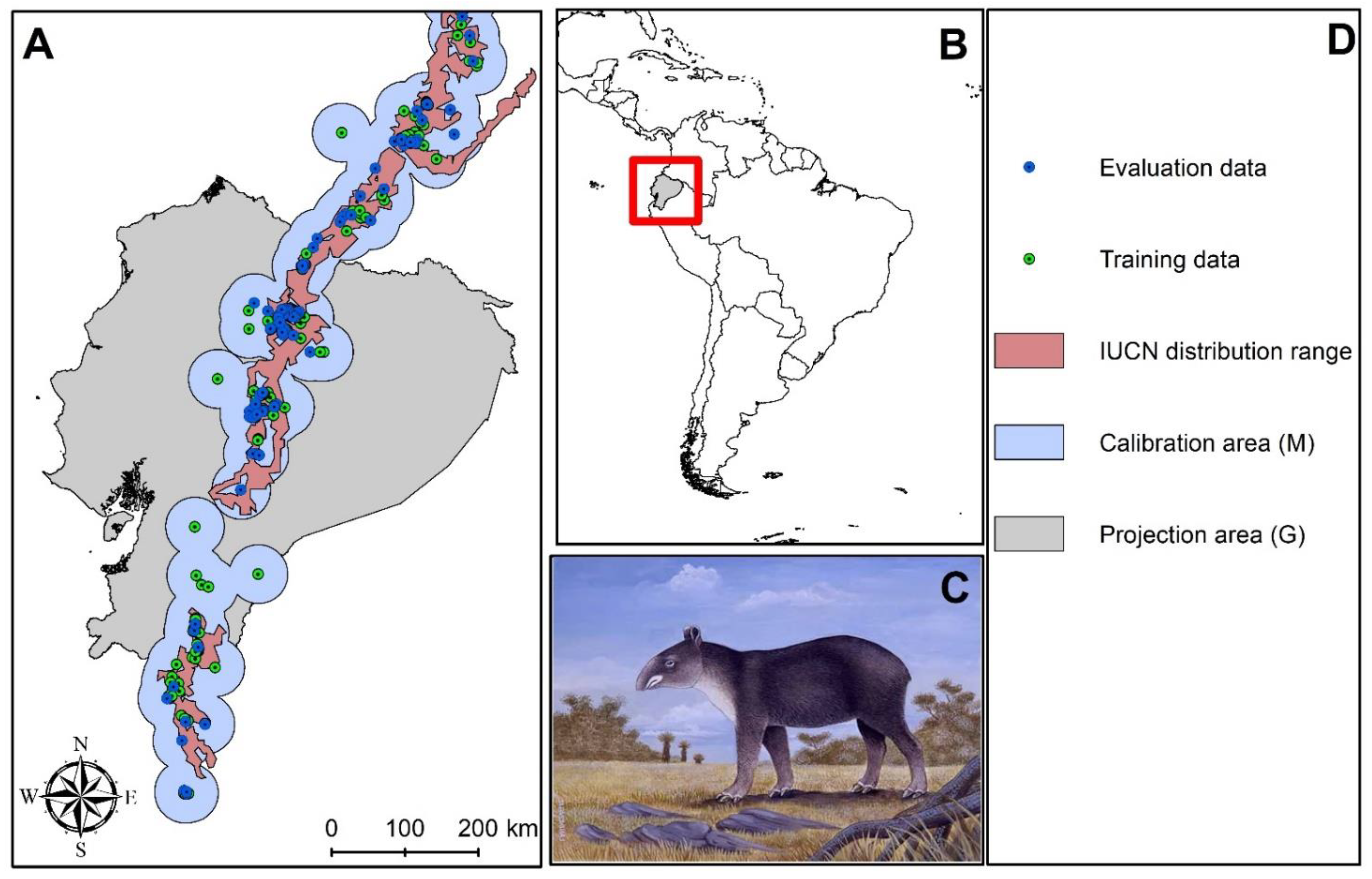
2.1. Study Area

The study area considered in this research for modeling purposes is centered on the Andes Mountains of Ecuador, with exact distribution zones of T. pinchaque, i.e., the Andean ecosystems, such as western montane forest, paramo, inter-Andean scrubland, and the eastern montane forest in Ecuador (Figure 1). This zone includes 19 provinces: Napo, Morona Santiago, Azuay, Bolívar, Cañar, Carchi, Chimborazo, Cotopaxi, El Oro, Esmeraldas, Loja, Orellana, Pastaza, Pichincha, Santo Domingo de los Tsachilas, Sucumbíos, Tungurahua, and Zamora Chinchipe [30,39].

2.2. Methods

For a better illustration and understanding, the methodological process is described, considering the objectives established in this study. Initially, a step-by-step description is given of the process followed for the generation of distribution models for the species under study. Then, the process adopted to quantify the predicted suitable areas for T. pinchaque in the SNAP of Ecuador is described. Finally, we describe the process used to estimate changes in suitable areas by comparing the current and future models for T. pinchaque in the study area.

2.2.1. Predictive Model

Occurrence Data

A database with validated occurrence records for T. pinchaque was constructed from the scientific literature, established within its native distribution limits, specifically for three Andean countries: Ecuador, Colombia, and Peru [29,40]. These records were previously obtained from biodiversity databases, such as GBIF (GBIF; www.gbif.org, accessed on 15 September 2021), MaNIS (www.manisnet.org), and the Tapir Specialist Group (IUCN/SSC TSG-Ecuador). In addition, occurrence records of T. pinchaque obtained through field work and monitoring projects in Colombia, Peru and Ecuador were included; a total of 1424 presence records were initially included in the database, including records from 1950 to the present (Supplementary Materials). Each occurrence record was projected on the geography through its coordinates (longitude, latitude) in decimal degrees based on the WGS 84 datum; this process was carried out using ArcMap 10.5. Each locality was verified and validated, eliminating records that presented geographical inconsistencies. Then, a cleaning protocol was applied, based on the methodology of Simoes [41], considering the recommended standards for the creation of ecological models [42,43]. This consisted of the following steps: (1) removing duplicate records, (2) verifying records with geographic inconsistencies, and (3) reducing areas with a high density of records, linked to oversampling close to accessible areas (settlements, roads, rivers, etc.) [44,45], in order to mitigate spatial autocorrelation and overfitting in the models [46,47]. This process was performed using the spThin package in R [48], managing a minimum distance of 1 km between each record. In this context, the cleaned database included 366 presence records (Figure 1). Finally, the aforementioned records were randomly split into two datasets, evaluation (20%) and calibration (80%), using the split_data function of the ellipsemm package in R [41].

Environmental Data

Nineteen bioclimatic variables were used at a spatial resolution of ~1 km2 from Worldclim version 1.4 [49], available at (http://www.worldclim.org/, accessed on 15 September 2021). Four variables were excluded (Bio 8, 9, 18, and 19), because they introduce spatial errors associated with the combination of temperature and precipitation information [50]. To forecast suitable areas of T. pinchaque distribution in the future, we used layers derived from projections of general circulation models (GCMs), for the average period between 2041 and 2060 (2050). Three GCMs (CCSM4, HadGEM2-ES, and MIROC5) were selected considering the variability and uncertainty present in the mathematical models used to generate future climate data [51,52]. In addition, two representative concentration trajectories (RCP 4.5 and RCP 8.5) were used for each GCM. These trajectories represent conservative (RCP 4.5) and pessimistic (RCP 8.5) greenhouse gas (GHG) emissions [53].
The dimensionality of the environmental dataset was reduced to mitigate the effects of the existing spatial autocorrelation between them, applying a Pearson coefficient (r > 0.8) between pairs of variables; this process was performed using the GUI version of the ntbox package [54]. Highly correlated variables were removed based on the previously mentioned threshold. Finally, five variables were selected: Bio 1, 2, 3, 12, and 15.

Calibration Area

For ecological niche models, the delimitation of a calibration area (M) [55] is a crucial and cautious process, mainly because its size influences the predictions generated by the algorithms [56], which implies possible overfitting and overpredictions in areas suitable for the species [57]. In view of this, a search was initially conducted in the current literature on the factors that influence the mobility of T. pinchaque. The results corroborated that altitude is one of the factors that restrict its range of mobility [58], with reports for T. pinchaque at altitudes ranging from 1200 to 4700 masl [34,59,60].
Because of the above, a digital terrain model (DEM) was downloaded at a resolution of 250 m, derived from the Shuttle Radar Topographic Mission (SRTM). The DEM was reclassified to identify the areas present between 1200 to 4700 masl. A hypothesis was then made about the accessibility area (M), using a 40 km buffer. This facilitated the capture of the altitudinal range suitable for T. pinchaque (Figure 1). Finally, a projection area (G) was defined, taking into account Ecuador, and considering the capacity of the ecological niche models to be projected in space (different geographic zones from those used for calibration) and periods (years) [41,55].

Model Calibration

For the construction of the models, the maximum entropy algorithm implemented in MaxEnt [61], through the kuenm package [62], was used. Aware that this type of algorithm, used for creating ecological models, is susceptible to configurations and parameterizations [63], which can cause problems related to over-fits and over-predictions in the final results [57], a rigorous calibration process was applied. This calibration consisted in the creation of candidate models, using a single set of variables (Set 1), 13 different regularization multiplier (RM) values (0.1–1 with intervals of 0.1, 1–4 with intervals of 1), as well as 29 possible combinations of feature classes (FC) (l = linear, q = quadratic, p = product, t = threshold, and h = hinge). The imposed parameters and configurations allowed us to evaluate the level of complexity of the models [64].

Evaluation and Creation of Final Models

Three metrics were used to evaluate the candidate models, allowing for the selection of the model with the best performance and the most simplicity in terms of parameterization and configuration. Initially, the significance ratio was calculated using partial ROC [65], a variant that allows for the resolution of issues associated with the traditional AUC, which is not recommended in ecological niche models. The resulting partial receiver operating characteristic (ROC) values range between 1 and 2, with values greater than 1 indicating good model performance. As a result, the predictive capacity was determined using the omission rate (OR) with a 5 percent tolerance for error [66]. The OR function enables the estimation of the fraction of presences predicted to be absent or false negatives. The Akaike information criterion for small samples (AICc) was then used to determine complexity [64]. This metric enables the assessment of the effect of the number of parameterizations and configurations on the generation of overfitted or highly complex models. As a result, only models with delta AICc < 2 values were chosen. After selecting the best model, final models for T. pinchaque were created for the present and future using 100% of the presence data, 10,000 background points, a maximum of 500 interactions, and ten replicates with logistic output format.
Consequently, models were projected from the calibration area (M) to the projection area (G), both for the current context and for future models, with their respective CPRs. During the model projection process, MaxEnt was configured to prevent extrapolation, avoiding possible overpredictions [57] in the final models.
Finally, seven resulting models were obtained: (1) current model; (2) future model CCSM4 for RCP 4.5; (3) future model CCSM4 for RCP 8.5; (4) future model HadGEM2-ES for RCP 4.5; (5) future model HadGEM2-ES for RCP 8.5; (6) future model MIROC5 for RCP 4.5; and (7) future model MIROC5 for RCP 4.5. Each had their respective replicates. The median was applied to the replicates of each model for the present period and future scenarios. Subsequently, the median of the medians was calculated for each RCP, thus generating consensus models, which summarize the variability existing in all the GCMs used [67]. As a result of this process, three definitive models were obtained: (1) current model; (2) consensus model RCP 4.5; and (3) consensus model RCP 8.5. These models were converted to binary, applying a threshold of 5% allowable omission error, considering the calibration data [66].

2.2.2. Representativeness of Predicted Suitable Areas in Ecuador’s SNAP

The predicted suitable areas in the SNAP of Ecuador were quantified by applying an overlap between the models generated for T. pinchaque and a vector file of the SNAP of Ecuador. This file was obtained from the spatial data infrastructure of the Ministry of Environment, Water and Ecological Transition of Ecuador (http://ide.ambiente.gob.ec/mapainteractivo/, accessed on 15 September 2021). The overlapping process was carried out using ArcMap 10.5. It is important to highlight that the SNAP in the context of Ecuador is considered one of the most effective methods of in situ conservation, given that it allows the protection and preservation of sensitive ecosystems and the biodiversity present in them. In addition, one of the tangible results is the success in counteracting the effects associated with deforestation and soil changes [25]. Hence, it is important to carry out this process of quantification of the areas predicted by the models as a conservation strategy for T. pinchaque.

2.2.3. Habitat Changes in the Distribution

The current binary model and future consensus models for RCP 4.5 and 8.5 were compared to estimate both the proportion and relative number of stable, lost, and gained pixels for T. pinchaque in its predicted range. This allowed the generation of models that report areas with potential future gains, losses, and stability. This process was performed through the BIOMOD_RangeSize function incorporated in the biomod2 package in R [68].

3. Results

3.1. Model Validation

Using the combination of 29 feature classes, 13 regularization multipliers, and a single set of variables, 377 candidate models for T. pinchaque were created and evaluated. Finally, three candidate models were statistically significant and met the AICc criteria (Table 1). The best candidate model used in the creation of the final models had an AUC ratio: 1.246, showing that it is a model with excellent predictive power, with an OR = 0.045, AICc = 8443.803, and ∆AICc = 0, in addition to the following configurations and parameterizations: RM = 0.7 and FC = qp (Table 1).
Sensitivity values representing the fraction of correctly predicted presences or true positives achieved by the models were obtained. In this context, the rate of presences correctly predicted by the models was 99.7% (with one presence not predicted) taking as reference the calibration area (M). Finally, with respect to the models generated in the projection area (G), the hit rate was 95% (10 non-predicted presences). It should be noted that in order to evaluate the sensitivity, the models had to be previously converted into binary, while the threshold used was 5% of the omission error. The sensitivity values obtained demonstrate the predictive power that the models had in predicting the presence data of T. pinchaque.

3.2. Representativeness of Suitable Areas Predicted by the Models in the SNAP

3.2.1. Model 1: Current

Under current conditions, the model reported suitable areas of approximately 67,805 km2 in Ecuador. Of these areas, 33.7% (22,872 km2) are within the SNAP, in contrast to 66.3% (44,933 km2) outside the SNAP. Regarding the SNAP territory, suitable areas for T. pinchaque habitats are reported in 31 of 61 protected areas (PA) (Table 2); among which the following PAs stand out, due to their higher proportion: Sangay National Park (NP) (4920 km2), Cayambe Coca NP (4305 km2), Llanganates NP (2487 km2), Sumaco Napo Galeras NP (1760 km2), Ecological Reserve (ER) Antisana (1392 km2), and Podocarpus NP (1383 km2).

3.2.2. Model 2: Future

The study area was divided into three zones: north, center, and south (Figure 1). In addition, these models suggest potential losses, gains, and stability of suitable areas for T. pinchaque habitats (Figure 2). Among the remarkable results, it can be mentioned that by the year 2050, the RCPs suggest that a large part of the area will be maintained, with values of 98.8% (66,970 km2) under the RCP 4.5 model compared to 98.6% (66,880 km2) of stability for the RCP 8.5 model. The PAs with 100% adequate area stability are: Bellavista private protected area, Cajas National Park, La Bonita Municipal Conservation Area, Cajas National Park, Cordillera oriental del Carchi decentralized autonomous protected area, El Ángel Ecological Reserve, Boliche National Recreation Area, Ichubamba Yasepan private protected area, La Bonita Municipal Conservation Area, Marcos Pérez De Castilla Community Protected Area, Pasochoa Wildlife Refuge, Quimsacocha National Recreation Area, Tambillo Community Protected Area, and Yacuambi Municipal Protected Area.
On the other hand, with respect to losses, the models report changes of 1.2% (835 km2) and 1.4% (925 km2) in the RCP 4.5 and 8.5 models, respectively. This suggests that most of the suitable areas that will show reductions are between 1060 and 2464 masl. These losses are evident in eight SNAP PAs: Cayambe Coca National Park, Cofan Bermejo Ecological Reserve, El Quimi Biological Reserve, Llanganates National Park, Sangay National Park, Siete Iglesias Municipal Conservation Area, and Sumaco Napo-Galeras National Park. Notably, El Zarza Wildlife Refuge is the most affected PA with a total reduction of suitable areas for T. pinchaque in both RCP models.
In general, the models project gains in suitable areas along the western and central zone of the Andean region of Ecuador, specifically in pixels of values with a minimum of 1087 and a maximum of 5863 masl. These gains were reported in nine SNAP PAs, highlighting a more significant gain in both RCP models in the following PAs: Chimborazo Wildlife Production Reserve, Los Ilinizas Ecological Reserve, and Cotacachi Cayapas National Park.

4. Discussion

In this study, a modeling process was performed based on the recommended standards [42,43], which meant that possible errors associated with sampling bias and spatial aggregation could be mitigated [44,46]. The process was able to accommodate the dimensionality of the set of environmental variables, the use of different settings and parameterizations [62], and the complexity of the models [64]. In this context, the models obtained after the selection process were highly significant (p < 0.001), had low omission rates (OR = 0.045), and were less complex (AICc = 8443.803, ∆AICc = 0). This is a clear difference compared to previous studies [29,69], where an exhaustive process was not applied in the selection of configurations and parameterizations in the calibration process, which is known to be very important for the final results of the models [63].
The results reported by the model under current conditions show that there is 67,805 km2 of suitable area for T. pinchaque in the Andean region of Ecuador, with 33.7% within the current SNAP, which is an acceptable range for the conservation of the species. Globally, 7.45% of the planet’s land surface is interconnected through PAs [70], which have contributed to biodiversity monitoring and conservation. For this reason, the expansion or creation of new protected areas in Ecuador is considered key as a beneficial in situ conservation strategy [27], because it would improve the connection between natural spaces in which T. pinchaque habitats, thus mitigating the impact of climate change observed in these areas [71]. The model under current conditions establishes that ~66% is outside the SNAP, which indicates insufficient connectivity in its territory for the preservation of this iconic species as a means of sustaining biological richness [69]. Its ecological role in sensitive environments, such as the páramos, is vital because it is a seed disperser and an excellent bioindicator of the conservation status of the ecosystems [34,72,73]. An example that demonstrates its importance is the Llanganates–Sangay ecological corridor, which has improved connectivity between the Llanganates and Sangay national parks, which are protected areas that have suitable areas that serve as habitats for T. pinchaque [72,74].
With respect to future predictions, the models suggest losses of ~2% in areas suitable for T. pinchaque distribution; these values are different from those reported by Ortega-Andrade [31], where they predict losses approximately equal to 17%. These differences can be addressed by the different methodologies used in both studies. Ortega-Andrade uses an omission error of 10%, which implies a significant reduction of adequate areas compared to the 5% applied in this study. Furthermore, it should be noted that a key difference was the use of different configurations and parameterizations in the MaxEnt algorithm through the kuenm package [62], which helped us avoid models with high complexity [64]. Finally, future models in this study have provided estimates for the total loss of suitable areas for T. pinchaque in the El Zarza Wildlife Refuge which could be associated with the influence of climate change in Andean regions. Therefore, it is vital to start taking initiatives to improve the adaptation of the species in the future in this protected area.
On the other hand, in terms of area gain, the models suggest that the western and central zones of the Andean region in Ecuador would be favored by these changes. However, these gains are reported in areas with pixels that have altitude values higher than what is currently known as a habitat for the species [34,59,60]. This can be explained in two ways. The biological explanation suggests that there is a relationship between altitudinal range and biodiversity. For example, an increase in temperature would induce a displacement towards areas that were previously colder, where environmental circumstances may be more conducive to the adaptation of populations in the future [75]. In this context, the displacement of fauna towards higher altitudinal zones is a relatively rapid process [76], which is not the case with the transition of flora towards higher altitudinal ranges [77]. This implies that T. pinchaque, being an herbivorous mammal [60], will in the future be limited with respect to its diet by not being able to rely on vegetation corresponding to its feeding habits, which could eventually lead to poor adaptation to higher altitudinal floors. The second explanation is that these areas are possible over-prediction zones generated by the models [57], which could be associated with the influence of size on the calibration area (M) used [56]. It is important to note that there is currently no standard methodology to minimize the drawbacks of this, so it is recommended to interpret with caution the areas reported for the species in areas with altitudinal ranges above 4700 masl. However, these areas could not be ruled out entirely, as studies suggest that climate change will influence Andean areas with higher altitudes in Ecuador [78,79], leading them to become increasingly abundant [78,80,81,82,83].
Multiple recommendations have been made in recent decades to improve the quality of niche models [34,35], including adequate cleaning of presence registers [33], delimitation of the calibration area (M) [48,49], incorporating a wide selection of parameters and configurations to minimize model complexity [56], and the use of multiple statistical criteria during the evaluation process [54]. These recommendations were taken into account when developing the final models, resulting in the generation of robust models at the predictive level. This study provides a deeper understanding of T. pinchaque’s distribution in Ecuador’s tropical Andes, and provides information on the species’ conservation status at a geographic scale, allowing for the identification of areas vulnerable and susceptible to future climate change effects. The study’s primary limitation was using only bioclimatic variables in the model generation process; this is justified because biotic interactions are imperceptible at coarse scales, such as those used in this study. Nonetheless, it is recommended that researchers continue developing models for T. pinchaque at finer scales using diverse environmental datasets (e.g., [73,74,75]) and global circulation models. Additionally, it would be necessary to analyze T. pinchaque’s biotic interactions with other mammalian species, their feeding patterns, the impact of land use change, and various anthropogenic activities.

5. Conclusions

Ecological niche models based on a rigorous selection and evaluation protocol were successfully used. The MaxEnt algorithm was used to estimate the potentially suitable areas for the distribution of T. pinchaque in current and future conditions. Robust models with excellent performance were obtained, considering the best configurations and parameterizations from the evaluation process. The geographic information presented in this study can be used in the short term to establish mitigation and adaptation strategies for climate change, to aid the design and establishment of connectivity zones between protected areas, and to evaluate biotic interactions with other tropical Andean species and environmental education programs based on the importance of the species in the conservation of Andean ecosystems in Ecuador.
Under current conditions, the models report suitable areas for the distribution of T. pinchaque in 19 provinces in Ecuador and 31 areas of Ecuador, representing a total of 67,805 km2. Under future conditions, these areas would remain stable, being equivalent to ~98% in both RCPs. In addition, future models report partial losses of suitable areas in seven protected areas and total losses in the El Zarza Wildlife Refuge, suggesting that environmental changes induced by future climate change will influence the species habitat. However, there are also estimated gains of suitable areas in nine protected areas, which allows us to analyze the importance associated with the increase in the proportion of protected areas in the SNAP of Ecuador for the conservation of T. pinchaque in the future.
The main threat identified for the tapir is the destruction of its habitat due to land use changes. With the projections made, we can show that, to a great extent, the in situ conservation strategy, i.e., the protected areas, play an essential role in the conservation processes of the species. However, it is essential to urge wildlife authorities and managers to join efforts to create strategies that contribute to connecting the main tapir habitats, such as, for example, biological corridors. This will facilitate the linking of dispersed populations, increasing the number of individuals and improving their genetic variability. Finally, it is important to continue with more studies that contribute to biodiversity conservation, considering the importance of balance in ecosystems to the humans dependent thereof.

Supplementary Materials

The following are available online at https://www.mdpi.com/article/10.3390/su132011486/s1.

Author Contributions

Conceptualization, C.M.-R., R.J.H.F., C.C.-O., I.D.G. and R.G.M.; methodology, C.M.-R. and R.J.H.F.; formal analysis, C.M.-R., R.J.H.F., C.C.-O., I.D.G. and R.G.M.; investigation, C.M.-R., R.J.H.F., C.C.-O., I.D.G. and R.G.M.; resources, C.M.-R., C.C.-O. and I.D.G.; writing—original draft preparation, C.M.-R., R.J.H.F. and C.C.-O.; writing—review and editing, C.M.-R., R.J.H.F. and C.C.-O.; visualization, C.M.-R., R.J.H.F., C.C.-O., I.D.G. and R.G.M.; supervision, C.M.-R.; project administration, C.M.-R. All authors have read and agreed to the published version of the manuscript.

Funding

This research was funded by Instituto Tecnológico Superior Universitario Oriente (Grant No. 34323674).

Institutional Review Board Statement

Not applicable.

Informed Consent Statement

Not applicable.

Data Availability Statement

Not applicable.

Acknowledgments

The authors would like to thank each of the researchers who carried out fieldwork for the georeferencing of data on the presence of Tapirus pinchaque in the tropical Andes.

Conflicts of Interest

The authors declare no conflict of interest.

References

  1. Nakamura, G.; Gonçalves, L.O.; da Silva Duarte, L. Revisiting the dimensionality of biological diversity. Ecography 2020, 43, 539–548. [Google Scholar] [CrossRef] [Green Version]
  2. Dunn, C.P. Biological and cultural diversity in the context of botanic garden conservation strategies. Plant Divers. 2017, 39, 396–401. [Google Scholar] [CrossRef]
  3. Woodward, G.; Bohan, D.A. Ecosystem Services: From Biodiversity to Society; Part 2; Elsevier: Amsterdam, The Netherlands, 2015. [Google Scholar]
  4. Balvanera, P.; Quijas, S.; Karp, D.S.; Ash, N.; Bennett, E.M.; Boumans, R.; Brown, C.; Chan, K.M.A.; Chaplin-Kramer, R.; Halpern, B.S. Ecosystem Services. In The GEO Handbook on Biodiversity Observation Networks; Walters, M., Scholes, R.J., Eds.; Springer International Publishing: Cham, Switzerland, 2017; pp. 39–78. [Google Scholar]
  5. Vimal, R.; Navarro, L.M.; Jones, Y.; Wolf, F.; Le Moguédec, G.; Réjou-Méchain, M. The global distribution of protected areas management strategies and their complementarity for biodiversity conservation. Biol. Conserv. 2021, 256, 109014. [Google Scholar] [CrossRef]
  6. Wilson, M.; Liu, S. Evaluating the non-market value of ecosystem goods and services provided by coastal and nearshore marine systems. In Ecological Economics of the Oceans and Coasts; Edward Elgar Publishing: Cheltenham, UK, 2008. [Google Scholar]
  7. Hernández-Blanco, M.; Costanza, R.; Anderson, S.; Kubiszewski, I.; Sutton, P. Future scenarios for the value of ecosystem services in Latin America and the Caribbean to 2050. Curr. Res. Environ. Sustain. 2020, 2, 100008. [Google Scholar] [CrossRef]
  8. Soley, F.G.; Perfecto, I. A way forward for biodiversity conservation: High-quality landscapes. Trends Ecol. Evol. 2021, 36, 770–773. [Google Scholar] [CrossRef]
  9. Pielke, R.A.; Adegoke, J.; Hossain, F.; Niyogi, D. Environmental and Social Risks to Biodiversity and Ecosystem Health—A Bottom-Up, Resource-Focused Assessment Framework. Earth 2021, 2, 440–456. [Google Scholar] [CrossRef]
  10. Dueñas, M.-A.; Hemming, D.J.; Roberts, A.; Diaz-Soltero, H. The threat of invasive species to IUCN-listed critically endangered species: A systematic review. Glob. Ecol. Conserv. 2021, 26, e01476. [Google Scholar] [CrossRef]
  11. Mantyka-Pringle, C.S.; Visconti, P.; di Marco, M.; Martin, T.G.; Rondinini, C.; Rhodes, J.R. Climate change modifies risk of global biodiversity loss due to land-cover change. Biol. Conserv. 2015, 187, 103–111. [Google Scholar] [CrossRef] [Green Version]
  12. Waldron, A.; Miller, D.C.; Redding, D.; Mooers, A.; Kuhn, T.S.; Nibbelink, N.; Roberts, J.T.; Tobias, J.A.; Gittleman, J.L. Reductions in global biodiversity loss predicted from conservation spending. Nature 2017, 551, 364–367. [Google Scholar] [CrossRef] [PubMed]
  13. Githiru, M.; Njambuya, J.W. Globalization and Biodiversity Conservation Problems: Polycentric REDD+ Solutions. Land 2019, 8, 35. [Google Scholar] [CrossRef] [Green Version]
  14. Mori, A.S.; Dee, L.E.; Gonzalez, A.; Ohashi, H.; Cowles, J.; Wright, A.J.; Isbell, F. Biodiversity–productivity relationships are key to nature-based climate solutions. Nat. Clim. Chang. 2021, 11, 543–550. [Google Scholar] [CrossRef]
  15. Marta, S.; Brunetti, M.; Manenti, R.; Provenzale, A.; Ficetola, G.F. Climate and land-use changes drive biodiversity turnover in arthropod assemblages over 150 years. Nat. Ecol. Evol. 2021, 5, 1291–1300. [Google Scholar] [CrossRef] [PubMed]
  16. Cuenca, P.; Arriagada, R.; Echeverría, C. How much deforestation do protected areas avoid in tropical Andean landscapes? Environ. Sci. Policy 2016, 56, 56–66. [Google Scholar] [CrossRef]
  17. Schwartz, K.R.; Gusset, M.; Crosier, A.E.; Versteege, L.; Eyre, S.; Tiffin, A.; otzé, A. The Role of Zoos in Tree Kangaroo Conservation: Connecting Ex Situ and In Situ Conservation Action. In Biodiversity of World: Conservation from Genes to Landscapes; Dabek, L., Valentine, P., Blessington, J., Schwartz Krbt, T.K., Eds.; Academic Press: Cambridge, MA, USA, 2021; Chapter 22; pp. 329–361. [Google Scholar]
  18. O’Connor, B.; Bojinski, S.; Röösli, C.; Schaepman, M.E. Monitoring global changes in biodiversity and climate essential as ecological crisis intensifies. Ecol. Inform. 2020, 55, 101033. [Google Scholar] [CrossRef]
  19. Fei, S.; Jo, I.; Guo, Q.; Wardle, D.A.; Fang, J.; Chen, A.; Brockerhoff, E.G. Impacts of climate on the biodiversity-productivity relationship in natural forests. Nat. Commun. 2018, 9, 5436. [Google Scholar] [CrossRef]
  20. Cheng, H.; Sinha, A.; Cruz, F.W.; Wang, X.; Edwards, R.L.; d’Horta, F.M.; Auler, A.S. Climate change patterns in Amazonia and biodiversity. Nat. Commun. 2013, 4, 1411. [Google Scholar] [CrossRef]
  21. Visscher, A.M.; Vanek, S.; Meza, K.; de Goede, R.G.; Valverde, A.A.; Ccanto, R.; Fonte, S.J. Eucalyptus and alder field margins differ in their impact on ecosystem services and biodiversity within cropping fields of the Peruvian Andes. Agric. Ecosyst. Environ. 2020, 303, 107107. [Google Scholar] [CrossRef]
  22. Fastré, C.; Possingham, H.P.; Strubbe, D.; Matthysen, E. Identifying trade-offs between biodiversity conservation and ecosystem services delivery for land-use decisions. Sci. Rep. 2020, 10, 7971. [Google Scholar] [CrossRef]
  23. Cunalata García, A.; López Pumalema, J. Turismo de humedales en Ecuador: Análisis a los sitios RAMSAR. Green World J. 2020, 3, 1–12. Available online: https://www.greenworldjournal.com/doi-018-ac-2020 (accessed on 15 September 2021).
  24. Bax, V.; Francesconi, W. Conservation gaps and priorities in the Tropical Andes biodiversity hotspot: Implications for the expansion of protected areas. J. Environ. Manag. 2019, 232, 387–396. [Google Scholar] [CrossRef]
  25. Acha, S.; Linan, A.; MacDougal, J.; Edwards, C. The evolutionary history of vines in a neotropical biodiversity hotspot: Phylogenomics and biogeography of a large passion flower clade (Passiflora section Decaloba). Mol. Phylogenetics Evol. 2021, 164, 107260. [Google Scholar] [CrossRef] [PubMed]
  26. Wong, W.S. Not the Same: Rethinking Chineseness in a Global Context Through Poster Design. In The Disappearance of Hong Kong in Comics, Advertising and Graphic Design; Wong, W.S., Ed.; Springer International Publishing: Cham, Switzerland, 2018; pp. 215–239. [Google Scholar]
  27. Mestanza-Ramón, C.; Henkanaththegedara, S.M.; Vásconez Duchicela, P.; Vargas Tierras, Y.; Sánchez Capa, M.; Constante Mejía, D.; Jimenez Gutierrez, M.; Charco Guamán, M.; Mestanza Ramón, P. In-Situ and Ex-Situ Biodiversity Conservation in Ecuador: A Review of Policies, Actions and Challenges. Diversity 2020, 12, 315. [Google Scholar] [CrossRef]
  28. Graham, R.W.; Grady, F.; Ryan, T.M. Juvenile Pleistocene tapir skull from Russells Reserve Cave, Bath County, Virginia: Implications for cold climate adaptations. Quat. Int. 2019, 530–531, 35–41. [Google Scholar] [CrossRef]
  29. Lizcano, D.J.; Cavelier, J. Using GPS collars to study mountain tapirs (Tapirus pinchaque) in the Central Andes of Colombia. Tapir. Conserv. 2004, 13, 18–23. [Google Scholar]
  30. Heredia, A.; Achoa, O.; Sandoval-Cañas, L.; Iglesias, M. Reportes sobre la presencia del Tapir de Montaña (Tapirus pinchaque) en el Parque Nacional Llanganates, Ecuador. Tapir. Conserv. 2007, 19, 1813–2286. [Google Scholar]
  31. Ortega-Andrade, H.M.; Prieto-Torres, D.A.; Gómez-Lora, I.; Lizcano, D.J. Ecological and Geographical Analysis of the Distribution of the Mountain Tapir (Tapirus pinchaque) in Ecuador: Importance of Protected Areas in Future Scenarios of Global Warming. PLoS ONE 2015, 10, e0121137. [Google Scholar] [CrossRef] [Green Version]
  32. Downer, C.C. Observations on the diet and habitat of the mountain tapir (Tapirus pinchaque). J. Zool. 2001, 254, 279–291. [Google Scholar] [CrossRef]
  33. Lizcano, D.J.; Cavelier, J. Daily and seasonal activity of the mountain tapir (Tapirus pinchaque) in the Central Andes of Colombia. J. Zool. 2000, 252, 429–435. [Google Scholar] [CrossRef]
  34. Lizcano, D.J.; Cavelier, J. Densidad Poblacional y Disponibilidad de Híbitat de la Danta de Montaña (Tapirus pinchaque) en los Andes Centrales de Colombia. Biotropica 2000, 32, 165–173. [Google Scholar] [CrossRef]
  35. Paz Mena, Y.S. Contaminación marina por actividades antrópicas. Green World J. 2018, 1, 1. [Google Scholar]
  36. Castellanos-Peñafiel, A.X.; Brito, J.; Castellanos-Insuasti, F.X. Tapirus pinchaque in Southwestern Ecuador. Serie Zoológica 2020, 16, 1–4. [Google Scholar]
  37. Herrera-Feijoo, R.J.; de Decker, M.; Chicaiza-Ortiz, C.; Penafilel Arcos, P.; Garzon Ortega, C. Posibles cambios en el rango de distribución de Tapirus pinchaque bajo escenarios de cambio climático. Green World J. 2021, 4, 1–19. [Google Scholar] [CrossRef]
  38. Alzate, A.A.; Downer, C.C.; Delgado, C.A.; Sánchez-Londoño, J.D. Un registro de tapir de montaña (Tapirus Pinchaque) en el norte de la Cordillera Occidental de Colombia. Mastozoología Neotropical 2010, 17, 111–116. [Google Scholar]
  39. Willis, S.G.; Hole, D.G.; Huntley, B. Climate Change and Conservation. In Trade-offs in Conservation: Deciding What to Save; Wiley-Blackwell: Hoboken, NJ, USA, 2010; pp. 329–348. [Google Scholar]
  40. Branco, V.V.; Cardoso, P. An expert-based assessment of global threats and conservation measures for spiders. Glob. Ecol. Conserv. 2020, 24, e01290. [Google Scholar] [CrossRef]
  41. Baker-Médard, M.; Gantt, C.; White, E.R. Classed conservation: Socio-economic drivers of participation in marine resource management. Environ. Sci. Policy 2021, 124, 156–162. [Google Scholar] [CrossRef]
  42. Fonseca, C.R.; Paterno, G.B.; Guadagnin, D.L.; Venticinque, E.M.; Overbeck, G.E.; Ganade, G.; Metzger, J.P.; Kollmann, J.; Sauer, J.; Cardoso, M.Z. Conservation biology: Four decades of problem- and solution-based research. Perspect. Ecol. Conserv. 2021, 19, 121–130. [Google Scholar] [CrossRef]
  43. Loaiza, P.J.A.; Cordova, P.A.A.; Valverde, F.M.V.; Ordóñez, D.A.T.; Torres, A.C.E.; Moretta, P.Y. El Tapir de montaña (Tapirus pinchaque), como especie bandera en los Andes del sur del Ecuador. INNOVA Res. J. 2017, 2, 86–103. [Google Scholar] [CrossRef]
  44. Simoes, M.; Romero-Alvarez, D.; Nuñez-Penichet, C.; Jiménez, L.; Cobos, M.E. General theory and good practices in ecological niche modeling: A basic guide. Biodivers. Inform. 2020, 15, 67–68. [Google Scholar] [CrossRef]
  45. Araújo, M.B.; Anderson, R.P.; Barbosa, A.M.; Beale, C.M.; Dormann, C.F.; Early, R.; Garcia, R.A.; Guisan, A.; Maiorano, L.; Naimi, B. Standards for distribution models in biodiversity assessments. Sci. Adv. 2019, 5, eaat4858. [Google Scholar] [CrossRef] [Green Version]
  46. Zurell, D.; Franklin, J.; König, C.; Bouchet, P.J.; Dormann, C.F.; Elith, J.; Fandos, G.; Feng, X.; Guillera-Arroita, G.; Guisan, A. A standard protocol for reporting species distribution models. Ecography 2020, 43, 1261–1277. [Google Scholar] [CrossRef]
  47. Zizka, A.; Antonelli, A.; Silvestro, D. Sampbias, a method for quantifying geographic sampling biases in species distribution data. Ecography 2021, 44, 25–32. [Google Scholar] [CrossRef]
  48. Gábor, L.; Moudrý, V.; Barták, V.; Lecours, V. How do species and data characteristics affect species distribution models and when to use environmental filtering? Int. J. Geogr. Inf. Sci. 2020, 34, 1567–1584. [Google Scholar] [CrossRef]
  49. Boria, R.A.; Olson, L.E.; Goodman, S.M.; Anderson, R.P. Spatial filtering to reduce sampling bias can improve the performance of ecological niche models. Ecol. Model. 2014, 275, 73–77. [Google Scholar] [CrossRef]
  50. Lobo, J.M. Debemos fiarnos de los modelos de distribución de especies? In Los Bosques y la Biodiversidad Frente al Cambio Climático: Impactos, Vulnerabilidad y Adaptación en España; Ministerio de Agricultura, Alimentación y Medio Ambiente: Madrid, Spain, 2015; pp. 407–417. [Google Scholar]
  51. Aiello-Lammens, M.E.; Boria, R.A.; Radosavljevic, A.; Vilela, B.; Anderson, R.P. spThin: An R package for spatial thinning of species occurrence records for use in ecological niche models. Ecography 2015, 38, 541–545. [Google Scholar] [CrossRef]
  52. Hijmans, R.J.; Cameron, S.E.; Parra, J.L.; Jones, P.G.; Jarvis, A. Very high resolution interpolated climate surfaces for global land areas. Int. J. Climatol. J. R. Meteorol. Soc. 2005, 25, 1965–1978. [Google Scholar] [CrossRef]
  53. Escobar, L.E.; Lira-Noriega, A.; Medina-Vogel, G.; Peterson, A.T. Potential for spread of the white-nose fungus (Pseudogymnoascus destructans) in the Americas: Use of Maxent and NicheA to assure strict model transference. Geospat. Health 2014, 9, 221–229. [Google Scholar] [CrossRef] [PubMed]
  54. Flato, G.; Marotzke, J.; Abiodun, B.; Braconnot, P.; Chou, S.C.; Collins, W.; Cox, P.; Driouech, F.; Emori, S.; Eyring, V. Evaluation of climate models. In Climate Change 2013: The Physical Science Basis; Contribution of Working Group I to the Fifth Assessment Report of the Intergovernmental Panel on Climate Change; Cambridge University Press: Cambridge, UK, 2014; pp. 741–866. [Google Scholar]
  55. Zappa, G.; Shepherd, T.G. Storylines of atmospheric circulation change for European regional climate impact assessment. J. Clim. 2017, 30, 6561–6577. [Google Scholar] [CrossRef] [Green Version]
  56. Van Vuuren, D.P.; Edmonds, J.; Kainuma, M.; Riahi, K.; Thomson, A.; Hibbard, K.; Hurtt, G.C.; Kram, T.; Krey, V.; Lamarque, J.-F. The representative concentration pathways: An overview. Clim. Chang. 2011, 109, 5–31. [Google Scholar] [CrossRef]
  57. Osorio-Olvera, L.; Lira-Noriega, A.; Soberon, J.; Peterson, A.T.; Falconi, M.; Contreras-Díaz, R.G.; Martínez-Meyer, E.; Barve, V.; Barve, N. ntbox: An R package with graphical user interface for modelling and evaluating multidimensional ecological niches. Methods Ecol. Evol. 2020, 11, 1199–1206. [Google Scholar] [CrossRef]
  58. Mota-Vargas, C.; Encarnación-Luévano, A.; Ortega-Andrade, H.M.; Prieto-Torres, D.A.; Peña-Peniche, A.; Rojas-Soto, O.R. Una breve introducción a los modelos de nicho ecológico. In La Biodiversidad en un Mundo Cambiante: Fundamentos Teóricos y Metodológicos Para su Estudio Universidad Autónoma del Estado de Hidalgo/Libermex, Ciudad de México; Universidad Autónoma del Estado de Hidalgo: Pachuca, Mexico, 2019; pp. 39–63. [Google Scholar]
  59. Barve, N.; Barve, V.; Jiménez-Valverde, A.; Lira-Noriega, A.; Maher, S.P.; Peterson, A.T.; Soberón, J.; Villalobos, F. The crucial role of the accessible area in ecological niche modeling and species distribution modeling. Ecol. Model. 2011, 222, 1810–1819. [Google Scholar] [CrossRef]
  60. Mendes, P.; Velazco, S.J.E.; de Andrade, A.F.A.; Júnior, P.D.M. Dealing with overprediction in species distribution models: How adding distance constraints can improve model accuracy. Ecol. Model. 2020, 431, 109180. [Google Scholar] [CrossRef]
  61. Mena, J.L.; Yagui, H.; La Rosa, F.; Pastor, P.; Rivero, J.; Appleton, R. Topography and disturbance explain mountain tapir (Tapirus pinchaque) occupancy at its southernmost global range. Topography and disturbance explain mountain tapir (Tapirus pinchaque) occupancy at its southernmost global range. Mamm. Biol. 2020, 100, 231–239. [Google Scholar] [CrossRef]
  62. Padilla, M.; Dowler, R.C.; Downer, C.C. Tapirus pinchaque (Perissodactyla: Tapiridae). Mamm. Species 2010, 42, 166–182. [Google Scholar] [CrossRef]
  63. Tirira, D.G.; Urgilés-Verdugo, C.A.; Tapia, A.; Cajas-Bermeo, C.A.; Izurieta, X.; Zapata-Ríos, G. Tropical Ungulates of Ecuador: An Update of the State of Knowledge. In Ecology and Conservation of Tropical Ungulates in Latin America; Springer: Berlin/Heidelberg, Germany, 2019; pp. 217–271. [Google Scholar]
  64. Phillips, S.J.; Anderson, R.P.; Schapire, R.E. Maximum entropy modeling of species geographic distributions. Ecol. Model. 2006, 190, 231–259. [Google Scholar] [CrossRef] [Green Version]
  65. Cobos, M.E.; Peterson, A.T.; Barve, N.; Osorio-Olvera, L. kuenm: An R package for detailed development of ecological niche models using Maxent. PeerJ 2019, 7, e6281. [Google Scholar] [CrossRef] [PubMed] [Green Version]
  66. Hallgren, W.; Santana, F.; Low-Choy, S.; Zhao, Y.; Mackey, B. Species distribution models can be highly sensitive to algorithm configuration. Ecol. Model. 2019, 408, 108719. [Google Scholar] [CrossRef]
  67. Warren, D.L.; Seifert, S.N. Ecological niche modeling in Maxent: The importance of model complexity and the performance of model selection criteria. Ecol. Appl. 2011, 21, 335–342. [Google Scholar] [CrossRef] [Green Version]
  68. Peterson, A.T.; Papeş, M.; Soberón, J. Rethinking receiver operating characteristic analysis applications in ecological niche modeling. Ecol. Model. 2008, 213, 63–72. [Google Scholar] [CrossRef]
  69. Anderson, R.P.; Lew, D.; Peterson, A.T. Evaluating predictive models of species’ distributions: Criteria for selecting optimal models. Ecol. Model. 2003, 162, 211–232. [Google Scholar] [CrossRef]
  70. Campbell, L.P.; Luther, C.; Moo-Llanes, D.; Ramsey, J.M.; Danis-Lozano, R.; Peterson, A.T. Climate change influences on global distributions of dengue and chikungunya virus vectors. Philos. Trans. R. Soc. B Biol. Sci. 2015, 370, 20140135. [Google Scholar] [CrossRef]
  71. Thuiller, W.; Lafourcade, B.; Engler, R.; Araújo, M.B. BIOMOD—A platform for ensemble forecasting of species distributions. Ecography 2009, 32, 369–373. [Google Scholar] [CrossRef]
  72. Hoorn, C.; Guayasamin, J.M.; Ortega-Andrade, H.M.; Linder, P.; Bonaccorso, E. Celebrating Alexander von Humboldt’s 250th anniversary: Exploring bio-and geodiversity in the Andes (IBS Quito 2019). Front. Biogeogr. 2019, 11, 2. [Google Scholar] [CrossRef] [Green Version]
  73. Saura, S.; Bertzky, B.; Bastin, L.; Battistella, L.; Mandrici, A.; Dubois, G. Protected area connectivity: Shortfalls in global targets and country-level priorities. Biol. Conserv. 2018, 219, 53–67. [Google Scholar] [CrossRef]
  74. Dinerstein, E.; Olson, D.; Joshi, A.; Vynne, C.; Burgess, N.D.; Wikramanayake, E.; Hahn, N.; Palminteri, S.; Hedao, P.; Noss, R. An ecoregion-based approach to protecting half the terrestrial realm. BioScience 2017, 67, 534–545. [Google Scholar] [CrossRef]
  75. Loor, D.K.B. Dieta del tapir de montaña (Tapirus pinchaque) en tres localidades del corredor ecológico Llangantes–Sangay. Boletín Técnico Serie Zoológica 2019, 10, 1–11. [Google Scholar]
  76. Puig, C.R.; Alvear, G.R. Diversidad en formícidos y plantas vasculares en el Parque Nacional Yasuní, Ecuador. Boletín Técnico Serie Zoológica 2019, 12, 10–11. [Google Scholar]
  77. Arias-Gutiérrez, R.; Reyes-Puig, J.; Tapia, A.; Terán, A.; Rodríguez, X.; Bermudez, D.; López de Vargas-Machuca, K. Desarrollo local y conservación en la vertiente oriental andina: Corredor ecológico Llanganates-Sangay-valle del Anzu. Revista Amazónica Ciencia y Tecnología 2016, 5, 52–68. [Google Scholar]
  78. Freeman, B.G.; Song, Y.; Feeley, K.J.; Zhu, K. Montane species and communities track recent warming more closely in the tropics. bioRxiv 2020. [Google Scholar] [CrossRef]
  79. Carnicer, C.; Eisenlohr, P.V.; de A. Jácomo, A.T.; Silveira, L.; Alves, G.B.; Tôrres, N.M.; de Melo, F.R. Running to the mountains: Mammal species will find potentially suitable areas on the Andes. Biodivers. Conserv. 2020, 29, 1855–1869. [Google Scholar] [CrossRef]
  80. Cuesta, F.; Peralvo, M.; Merino-Viteri, A.; Bustamante, M.; Baquero, F.; Freile, J.F.; Muriel, P.; Torres-Carvajal, O. Priority areas for biodiversity conservation in mainland Ecuador. Neotrop. Biodivers. 2017, 3, 93–106. [Google Scholar] [CrossRef]
  81. Herzog, S.K.; Tiessen, H. Climate Change and Biodiversity in the Tropical Andes; Fundacion Ambiente y Recursos Naturales: Capital Federal, Argentina, 2017. [Google Scholar]
  82. Báez, S.; Jaramillo, L.; Cuesta, F.; Donoso, D.A. Effects of climate change on Andean biodiversity: A synthesis of studies published until 2015. Neotrop. Biodivers. 2016, 2, 181–194. [Google Scholar] [CrossRef]
  83. Peters, T.; Drobnik, T.; Meyer, H.; Rankl, M.; Richter, M.; Rollenbeck, R.; Thies, B.; Bendix, J. Environmental changes affecting the Andes of Ecuador. In Ecosystem Services, Biodiversity and Environmental Change in a Tropical Mountain Ecosystem of South Ecuador; Springer: Berlin/Heidelberg, Germany, 2013; pp. 19–29. [Google Scholar]
Figure 1. (A) Study area, represented in three zones: north, center, and south; (B) known distribution area of T. pinchaque in the South American Andean region; (C) infographic of the species; (D) Map legend.
Sustainability 13 11486 g001
Figure 2. Reported changes in areas suitable for T. pinchaque distribution under climate change scenarios.
Sustainability 13 11486 g002
Table 1. Performance of the best models under the parameters imposed in the calibration and evaluation process.
ModelAUC RatioORAICc∆AICcRMFC
11.2460.0458443.8030.0000.7qp
21.1730.0458445.1061.3030.8qp
31.1620.0458445.1851.3820.6qp
Features classes (FC), omission rate 5% (OR), Akaike information criterion-corrected (AICc), delta Akaike information criterion-corrected (∆AICc). q = quadratic; p = product.
Table 2. Predicted suitable areas (km2) for T. pinchaque within the National Protected Areas System of Ecuador.
Name of Protected AreaDesign TypeCurrent (km2)RCP 4.5 (km2)RCP 8.5 (km2)
AntisanaER13921406 (+1.01%)1408 (+1.15%)
BellavistaPPA33 (0%)3 (0%)
CajasNP350350 (0%)350 (0%)
Cayambe CocaNP43054235 (−1.63%)4300 (−0.12%)
Cerro PlateadoBR224235 (+4.91%)238 (+6.25%)
ChimborazoWPR388613 (+57.99%)621 (+60.05%)
Cofan BermejoER133129 (−3.01%)127 (−4.51%)
Colonso ChalupasBR976969 (−0.72%)980 (+0.41%)
Cordillera Oriental Del CarchiDAPA231231 (0%)231 (0%)
Cotacachi CayapasNP694757 (+9.08%)807 (+16.28%)
CotopaxiNP350374 (+6.86%)376 (+7.43%)
El ÁngelER187187 (0%)187 (0%)
El BolicheNRA66 (0%)6 (0%)
El QuimiBR102100 (−1.96%)98 (0%)
El ZarzaWR60 (−100.00%)0 (0%)
Ichubamba YasepanPPA5454 (0%)54 (0%)
La BonitaMCA621621 (0%)621 (0%)
LlanganatesNP24872473 (−0.56%)2479 (−0.32%)
Los IlinizasER745957 (+28.46%)1055 (+41.61%)
Marcos Pérez De CastillaCPA9999 (0%)99 (0%)
PasochoaWR44 (0%)4 (0%)
PodocarpusNP13831432 (+3.54%)1443 (+4.34%)
PululahuaGR3738 (+2.70%)38 (+2.70%)
QuimsacochaNRA3232 (0%)32 (0%)
Rio Negro SopladoraNP386386 (0%)385 (−0.26%)
SangayNP49204852 (−1.38%)4865 (−1.12%)
Siete IglesiasMCA175174 (−0.57%)171 (−2.29%)
Sumaco Napo-GalerasNP17601722 (−2.16%)1750 (−0.57%)
TambilloCPA2121 (0%)21 (0%)
YacuambiMCA307307 (0%)307 (0%)
YacuriNP494496 (+0.40%)497 (+0.61%)
Abbreviations: NP = national park; ER = ecological reserve; PPA = private protected area; BR = biological reserve; WPR = wildlife production reserve; DAPA = decentralized autonomous protected area; NRA = national recreation area; WR = wildlife refuge; MCA = municipal conservation area; CPA = community protected area; GR = geobotanic reserve.
Publisher’s Note: MDPI stays neutral with regard to jurisdictional claims in published maps and institutional affiliations.

