Techno-Economic Optimization of a Solar–Wind Hybrid System to Power a Large-Scale Reverse Osmosis Desalination Plant

Soliman, A. M.; Alharbi, Abdullah G.; Sharaf Eldean, Mohamed A.

doi:10.3390/su132011508

Open AccessArticle

Techno-Economic Optimization of a Solar–Wind Hybrid System to Power a Large-Scale Reverse Osmosis Desalination Plant

by

A. M. Soliman

^1,2,*,

Abdullah G. Alharbi

³ and

Mohamed A. Sharaf Eldean

²

¹

Department of Mechanical Engineering, College of Engineering, Jouf University, Sakaka 72388, Saudi Arabia

²

Department of Mechanical Engineering, Faculty of Engineering, Suez University, Suez 41522, Egypt

³

Department of Electrical Engineering, College of Engineering, Jouf University, Sakaka 72388, Saudi Arabia

^*

Author to whom correspondence should be addressed.

Sustainability 2021, 13(20), 11508; https://doi.org/10.3390/su132011508

Submission received: 14 September 2021 / Revised: 11 October 2021 / Accepted: 13 October 2021 / Published: 18 October 2021

Download

Browse Figures

Review Reports Versions Notes

Abstract

:

Solar-wind hybrid systems have grown to become a pivotal option for powering membrane desalination processes, especially because they have zero harmful emissions. In this work, solar photovoltaic (PV) and horizontal wind turbine (HWT) systems were used to drive a reverse osmosis (RO) desalination process to produce large-capacity fresh water. Moreover, an investigation into a hybrid PV–HWT system combined with RO was also conducted. The proposed systems are compared technically and economically with the solar organic Rankine cycle (SORC) for RO. Technical and analytical optimization methods were performed to minimize the unit product cost (USD/m³). The results revealed that photovoltaic-powered RO is recommended over wind energy operations. However, for large capacities, both thermal and wind farms dominate.

Keywords:

photovoltaic system; horizontal wind turbines; solar organic Rankine cycle; reverse osmosis

1. Introduction

The Middle East and North Africa (MENA) have the world’s lowest per capita availability of water resources [1]. Fortunately, most MENA countries have a renewable energy potential that encourages the application of solar and wind to drive desalination units. Renewable energy to drive the desalination units is a vital solution to water scarcity in remote areas that lack conventional energy sources like heat and electricity grid [2]. Reverse osmosis (RO) is a modern process to desalinate water for a wide range of applications [3].

For this technique, mechanical energy in the form of a high-pressure pump, not thermal energy, is required. In recent decades RO has gone through a remarkable development. The number of RO plants has increased and the capacity of the units has reached 3,000,000 m³/day [4]. The reliability and the availability of combining renewable energy resources such as solar and wind power are reasons for using RO instead of thermal distillation processes. Photovoltaic (PV) panels are the common form of solar energy generation in RO units. Essam Mohamed et al. [5] investigated technically and economically a photovoltaic system to drive RO desalination. The productivity of that system was 0.35 m³/day with a specific power consumption of about (4.6 kWh/m³). The cost of fresh water was about (EUR 15–20/m³), which is high because of the need for a large number of batteries to stabilize the pressure and flow rate for the membranes [5]. An economic feasibility study of PV power on RO within low specific power consumption was established by Helal [6]. It was conducted using three alternative configurations of an autonomous PV–RO unit in the United Arab Emirates (UAE). In that study, a diesel generator was used during periods of low sunlight. The productivity of PV-RO was not more than 20 m³/day (10 h). In Helal’s study, the environmental impacts of diesel generator emissions were ignored. The technical characteristics of PV-RO desalination systems and an economic comparison were presented by Manolakos [7]. The total peak power of the PV system was 846 W and consisted of 18 Arco-Solar mono-crystalline PV panels. The productivity of the system was 0.1 m³/h and the specific energy consumption has been found to be in the range of 3.8–6 kWh/m³. It is found that the cost of 1 m³ of fresh water was about EUR 7.77. Ahmed [8] found that the cost of the productivity for a PV-powered small-scale RO water desalination system is USD 3.73/m³. In Morocco, Tzen [9] studied an autonomous PV–RO system for the potable and other water needs of a rural community and found that the specific power consumption (SPC) was 15 kWh/m³).

Wind energy is also used in this kind of operation, and some of the literature is provided in this section. Liu et al. [10] studied a RO system driven by wind energy for wastewater treatment without an economic study. An experimental RO plant connected directly to a wind system without energy storage was presented by Pestana [11]. The system was designed based on 21 kW of power, to produce 3.6 m³/h. Dehmas et al. [12] found that wind energy can successfully power a desalination plant. Their studies included the economic analysis of 5 Bonus 2 MW wind turbines. Garcia-Rodriguez et al. [13] presented the influence of the climate, nominal power of the wind turbine, salt concentration, design arrangement, operating conditions, and plant capacity on the cost of fresh water. Romero-Ternero et al. [14] presented exergo-economic analysis for wind-powered seawater RO system the unit cost of freshwater was EUR 0.76/m³. Wind RO plants have a wide range capacity of 12–2500 m³/day with nominal power of 4–200 kW [15]. Dimitriou et al. [16], and Ruiz-García and Nuezb [17], investigated the performance of RO under variable operating conditions, and another study by Ruiz-García and Nuezb [18] investigated the long-term intermittent performance of a brackish water RO desalination plant.

From the literature review, the hybrid wind–PV system for driving RO has shown advantages: a wide range of capacities, minimal energy loss, easy maintenance and reliability. However, such systems were not investigated from a problem optimization or techno-economic perspective. Optimization criteria are very important because they reduce the total power consumption on the RO high-pressure pump (HPP), thereby, reducing the area of the solar field and the total cost. It is obvious from the literature that the possibility of producing a large water capacity (>3000 m³/day) is far away because of the cost limitations of PV and wind technologies. Furthermore, electric storage for PV and wind power is still unaffordable. In this study, under the steady regime, the design and optimization of the various capacities of a PV-horizontal wind turbine (HWT)–RO system are investigated to come to a clear decision about the feasibility of using PV and HWT regardless of location or weather condition. Moreover, the comparison between the proposed systems and the solar thermal power cycle of a RO operation is performed. The optimization of techno-economic issues is the focus of this work to decrease power consumption and system costs. The work proceeds as follows:

Process configurations are presented, design limits are investigated, and the mathematical model of the proposed systems is presented.
The optimization method is performed to study the effect of cost minimization.
A comparison of four cases (solar direct–three configurations vs. solar indirect–one configuration) is performed.

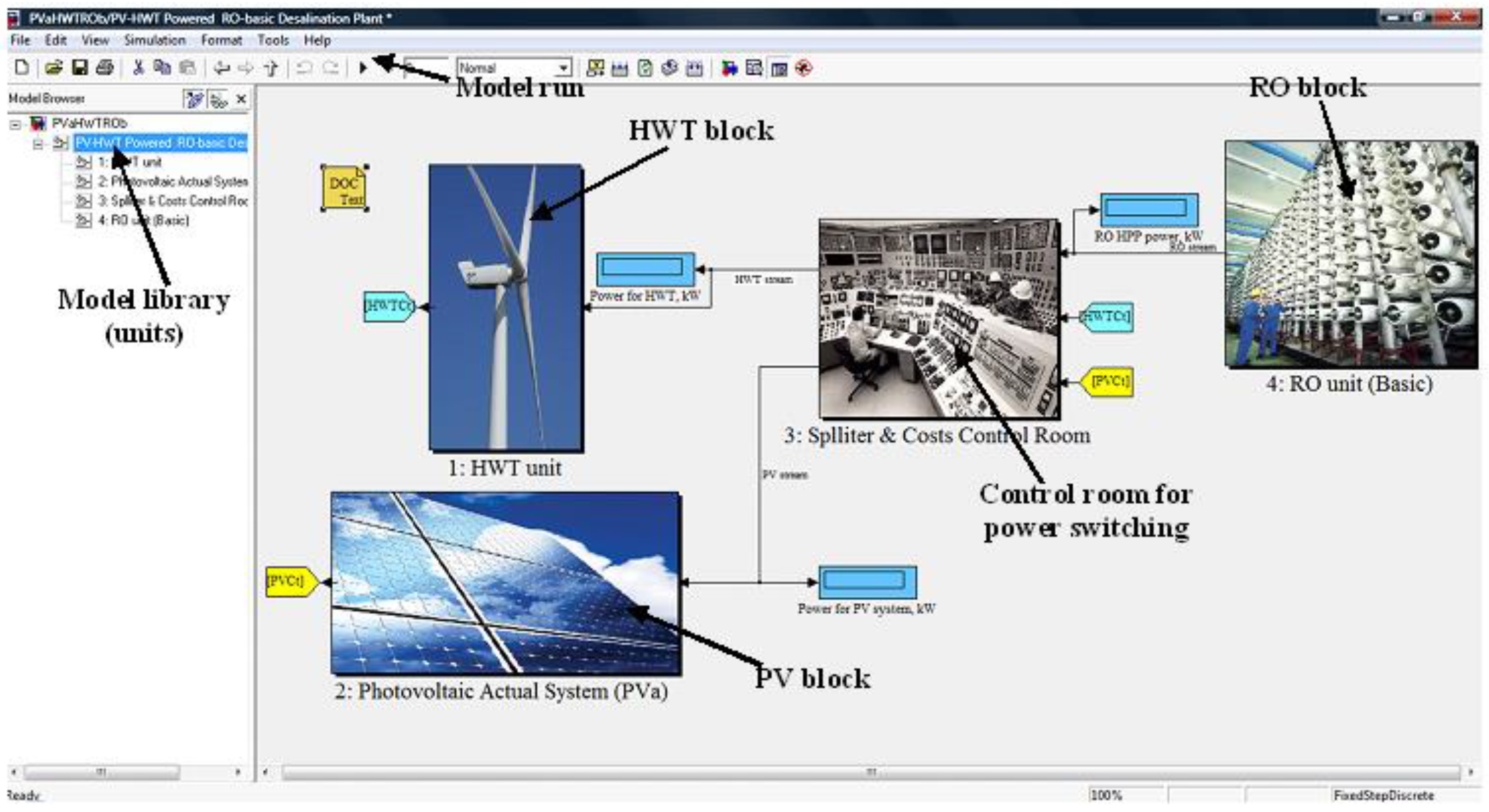
2. The Process Configurations

The combination of solar power with RO was achieved by one of two methods. The first is electrical (PV and HWT), and the second is via the thermal solar Rankine cycle. The proposed configuration related to the electrical method was modeled using SDS software and shown in Figure 1 [19]. SDS is a developed software library as a part of the REDS program library developed by Sharaf et al. [16]. The model configuration contained a PV, HWT, inverter unit, battery bank (storage unit) and a control room for power switching between PV and HWT to operate the RO system.

The RO unit was operated by HWT, PV or both (PV–HWT). Concentrated solar power (CSP) is shown in Figure 2. This configuration is presented based on thermal power to operate the organic Rankine cycle (ORC) to generate power to operate the RO system. This configuration contained a parabolic trough collector (PTC) field for the thermal power, a boiler heat-exchanger unit (BHX), pumps, ORC turbine, recuperator for regeneration and energy recovery, a condenser unit for heat rejection and the pre-heating of salt water stream and the RO system. Therminol-VP1 [20] was used as heat transfer oil (HTO) in the fourth configuration. Toluene was used as the working substance through the ORC [2,20,21].

3. Simulation Methodology

The calculated parameters were area, dimension, mass flow rate, and temperature. For the desalination, the fresh water capacity was specified, after which the electrical load was calculated for either PV or the HWT design specifications. The calculated parameters and design limits of the proposed units are illustrated in Table 1. The mathematical model representing the process configurations and validity is listed in the Appendix A.

4. Results and Comments

4.1. Non-Optimization Comparison Results

There are many ways to judge process performance results such as by field area, fresh water production rate, salinity range or specific costs. The main performance indicator studied in this work was the unit product cost (UPC) in USD/m³. This indicator is very important, giving an early evaluation before the optimization procedures. In this section, the process results are obtained at an RO production rate of 3500 m³/day as a pre-stage before optimization. The costs of the system units are illustrated in the Appendix A. The user has to specify total productivity and then all the required parameters will be calculated relatively and iteratively.

Table 2 shows the data results for the HWT-RO system for 3500 m³/day. The results revealed that to generate 1131 kWe, two 600-kWe HWTs were used. HWT-600 kW was used because the expected wind speed in the Suez Gulf region is suitable. The average wind speed is 11–12 m/s. Technical analyses showed that the hub height was about 41 m with a 43 m rotor diameter. The wind farm occupies about 0.063 km² of land; the total annual cost is about 6.31 × 10⁵ USD/year; and the unit product cost (UPC) is about 0.5541 USD/m³.

Table 3 presents the results of the PV–RO system that produced the same amount of fresh water (3500 m³/day). The expected power load was 1131 kWe for the RO plant, and a 220 W module is chosen for the PV site. In addition, 350 W/m² of solar radiation was chosen as a known input parameter to calculate the PV site area based on the worst winter conditions [22]. Excess power in summer could be stored in other facilities such as the control room cabinet or lighting issues in the plant. Compared to the HWT–RO, the PV–RO had a lower UPC (USD 0.53 vs. 0.55/m³) and a smaller solar field site (about 0.02 vs. 0.06 km²). Based on current results, the PV–RO system is considered to have a lower UPC than the HWT–RO system.

Table 4 shows the results of the hybrid system in which the power demanded by the RO plant is equally divided between the HWT farm and the PV site. The results revealed that the hybrid took up a larger area (HWT farm and PV site area) and the UPC increased to USD 0.5744/m³ due to the HWT number increase. It is obvious from the related tables that the UPC could be optimized to a minimum value with respect to the site area by selecting the right PV module power or the number of wind turbines. Moreover, the PV–RO system was considered attractive against the remaining systems according to the minimum area required and UPC in USD/m³. However, the 280 W module may consume a larger area with a higher cost per site. Therefore, optimization should be implemented to identify the greatest effect of each system on the UPC in USD/m³.

4.2. Comparison Results Based on Optimization

It was becoming very hard to recognize the main cause for the UPC. Previous results indicated that the PV–RO system had the lowest UPC; however, such a result needs more investigation based on many factors such as the number of wind turbines, modules of watts of PV, and RO operating conditions. For that purpose, technical and analytical optimization techniques were implemented. The technical method was implemented for the RO part, but the analytical method was implemented for the RO, HWT, and PV systems.

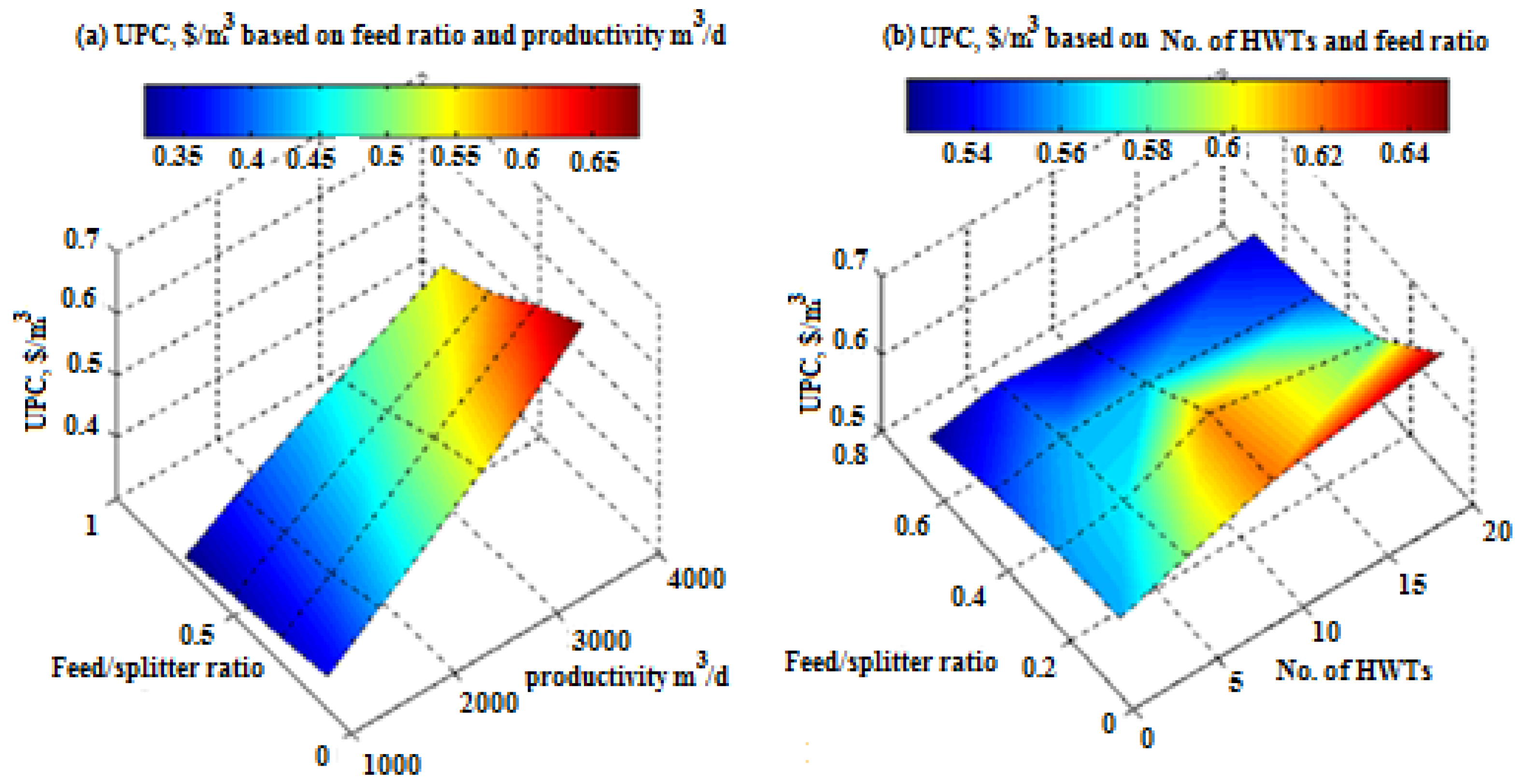
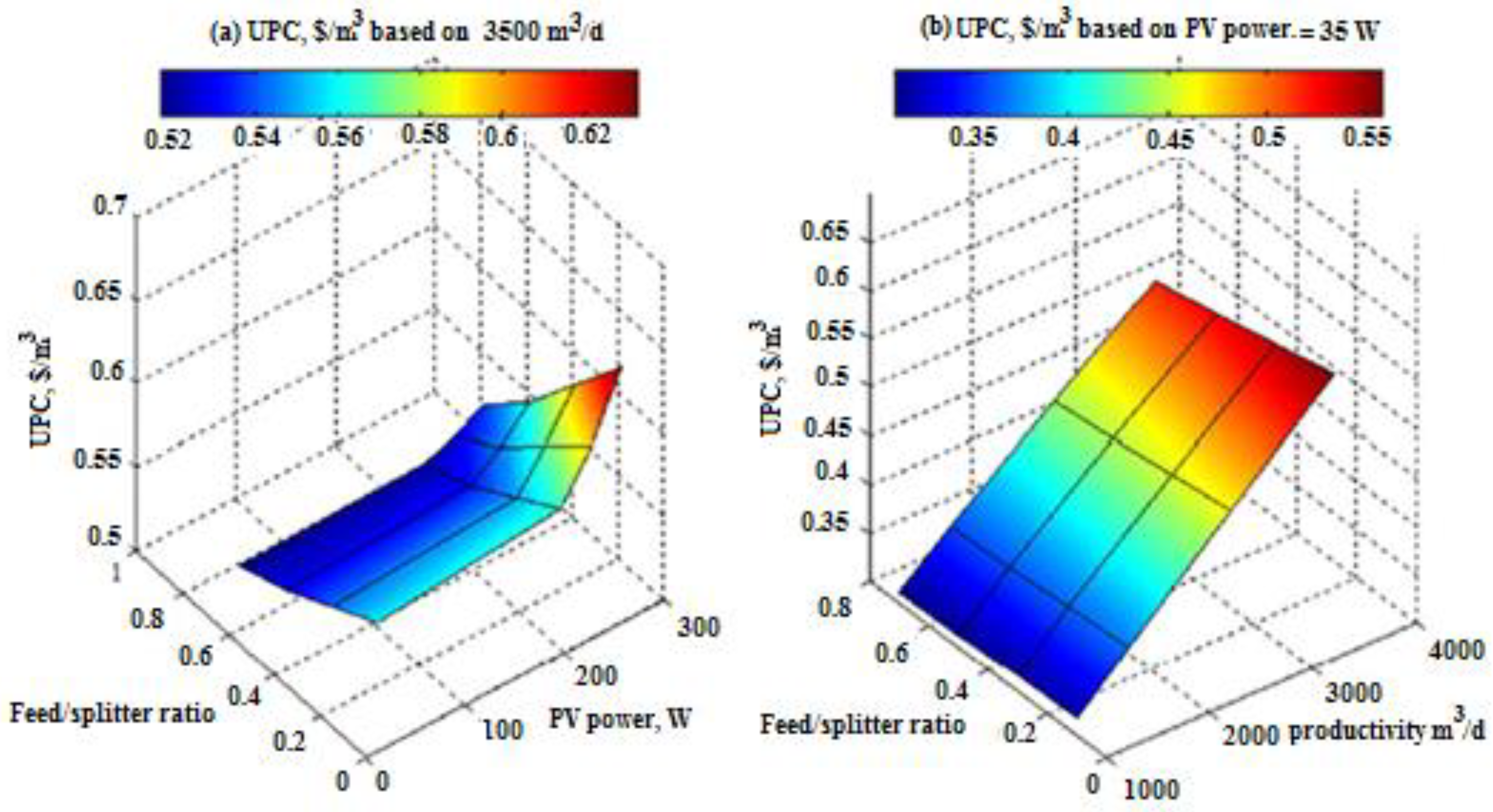
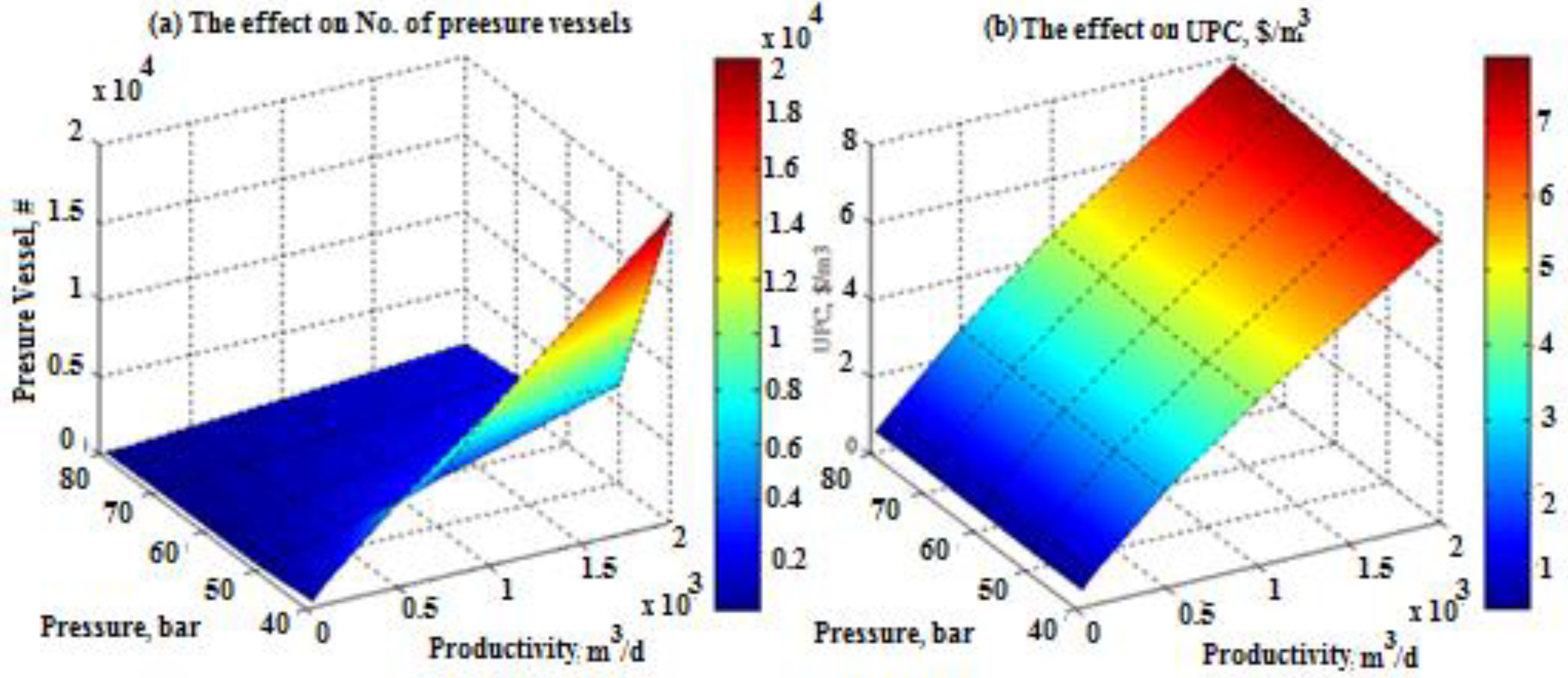
4.2.1. Technical Optimization Results

In this section, the solution to minimize the objective function (UPC, USD/m³) was implemented for the RO part. Optimizing it influenced the HWT and PV. To minimize the UPC, it was necessary to reduce the HPP power load and maintain the same fresh water production rate. Increasing the number of stages decreased the HPP power load. For the same case study (3500 m³/day), the number of stages was increased to nine. Table 5 shows that the increased number of stages decreased the power from 1131 to 917.47 kW (18–20%). Then the calculated SPC became 6.3 vs. 7.7 kWh/m³ in the basic case. Based on a previous study [3,21], increasing the number of stages decreased the HPP power load and the PEX device dominated operations in RO plants, reducing power consumption by 60–65% [22]. Table 5 shows the data results of the RO plant for 3500 m³/day based on the different technical devices. Therefore, the PEX device is recommended in this study.

4.2.2. The Analytical Optimization Results

Based on the technical results in the previous section, the RO-PEX technique is recommended for the analytical method. Figure 3 shows the effect of the RO-PEX inlet feed/splitter ratio and the total system productivity on the UPC. The figure addressed the case of HWT-RO-PEX without the operation of the PV solar field. Decreasing the inlet feed splitter ratio to 10% increased the demanded power by the HPP by more than three times (390 to 1532 kW). The UPC was directly proportional to this effect, increasing to 0.683 USD/m³ at 3500 m³/day. Furthermore, the effect on total productivity was also notable with respect to the feed/splitter ratio. The number of HWTs in the wind farm was a very important parameter that affected the UPC (Figure 3b). Increasing the number of wind turbines (low power per unit) increased the UPC. Therefore, fewer than two units are recommended for this operation.

Decreasing the quantity of total fresh water from 3500 to 1000 m³/day would also increase the UPC for the same operating conditions. At 3500 m³/day and a feed/splitter ratio of 70%, the UPC is about 0.548 USD/m³. Figure 4a,b represents the effect of the inlet feed splitter, PV module power, and total productivity on the UPC. Figure 4a,b demonstrates the effect on the UPC without the operation of the HWT farm. In Figure 4a, results are obtained at total productivity of 3500 m³/day. The figure shows that it was important to increase the feed/splitter ratio related to the RO-PEX part because it decreased the HPP power demand and hence lowered the UPC. At the same time, selecting a module with a higher rate of power increased the UPC. The results revealed that the PV 35 W module was the best choice with a feed/splitting ratio of more than 70%. However, the PV 280 W module increased the UPC. For a ratio of 70% and PV 35 W, it was about 0.517 USD/m³.

Figure 4b shows the effect of various system production rates from 1000 to 3500 m³/day on the UPC. The optimized point is obvious at 0.31 against 0.557 USD/m³. Decreasing total productivity while increasing the inlet feed/splitter ratio led to a decrease in the UPC. For the operation of the PV field, the 35 W module is effective because of the individual unit price. Moreover, increasing rather than decreasing the inlet feed/splitter ratio is recommended for the following reasons:

It decreases the electrical load on the HPP unit;
The operation proceeds without any need for more pressure vessels or membranes;
The gain power is fully loaded on the PEX unit without any excess power from the brine loss.

Suppose that the investor or the designer had to choose between the PV solar field or the HWT farm or both with respect to the control room load (CRL) distribution. From the results, the operation of the PV is recommended over the HWT operation based on the UPC. For both operations, increasing the load percentage meant increasing the dependent load on the HWT farm. Figure 5 shows the variations in the electric load distribution between the PV and the HWT. It is evident that the UPC was minimized by a load percentage of less than 5%; i.e., fully operated by the PV solar field. Decreasing the load on the HWT farm lowered the UPC. The operation with less than a 5% load on the HWT farm was remarkable and cost about USD 0.518/m³. Criteria to consider when selecting the type of operation are

The PV module power and number of HWTs,
The total productivity with respect to the inlet feed/splitter ratio, and
The site operating conditions, which decide the number of HWTs in the farm based on the power of each turbine.

According to Equations (A1) and (A14) in the Appendix A, increasing the power load depends on system productivity, and the feed mass flow rate and the HPP pressure depend on the design parameters of the RO modules. Therefore, the power is a multidimensional functional of parameters:

P o w e r = f {\begin{matrix} ∆ P = f (A_{e}, n_{e}, N_{V}, k_{w}, F F, T C F) \\ M_{f = f {\begin{matrix} M_{d} \\ R R \end{matrix}} \end{matrix}

(1)

where A_e, n_e, N_V are the design parameters for the RO, and their effect is notable on the RO pressure.

In this optimization, the constraints of the algorithm are FF = 0.85; TCF = f(T_f); A_e = 35.5 m²; n_e = 8 elements, and the limits of the system are changed around the M_d, N_V, and the

∆ P

. The results revealed that more productivity meant more power at the same recovery ratio (RR) of 0.3. It was obvious that by increasing system productivity up to 200,000 m³/day the N_V would directly affect the UPC at the same pressure category (e.g., 40 bar). The UPC increased from 0.47 to 7.33 USD/m³ by the use of 20,000 N_V. Increasing the N_V decreased the UPC by increasing the

∆ P

, thereby decreasing the power and the load on the PV site. For moderate production (10,000 m³/day), about 1450 pressure vessels at 40 bar were proposed; however, 750 pressure vessels to produce 100,000 m³/day at 80 bar were used. It is clear now that the choice should have been made according to the lower cost for each pressure category. Therefore, 40 bar should be used, but the massive number of pressure vessels is considered a hindrance to maintenance and system control. For less control and fewer maintenance issues 80 bar is preferred; moreover, maximum production could reach 200,000 m³/day with 1500 pressure vessels compared with 20,000 pressure vessels for 40 bar. According to the PV site, the operation of 200,000 m³/day is considered a massive challenge because of the relation of the site area to the PV site, which would have to generate about 24 MWe. Therefore, because of cost, the 40-bar category was favored in this study. Figure 6 shows the data results of the effect of pressure and productivity on the system pressure vessel numbers and UPC.

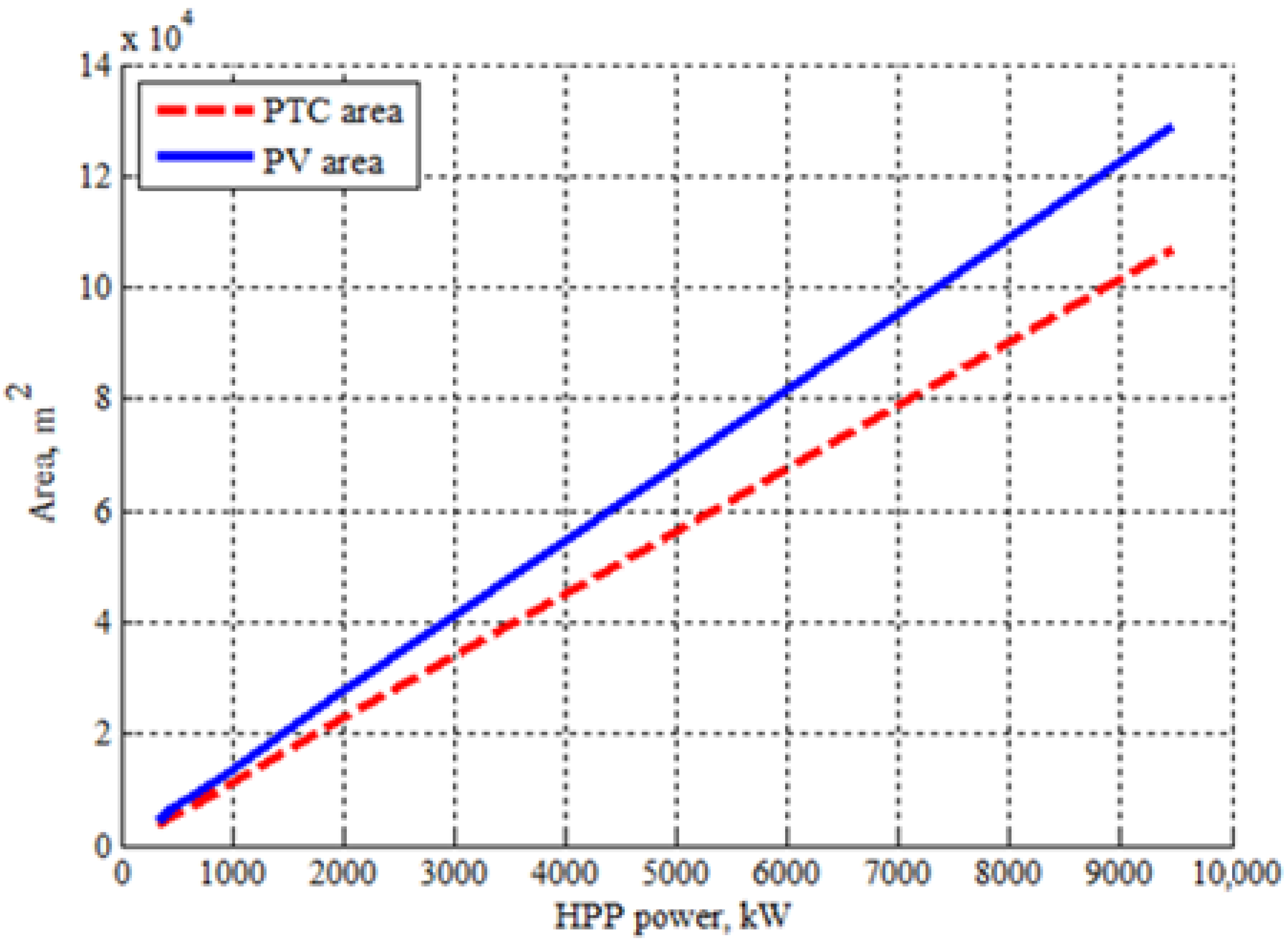
4.3. Data Results Compared with Solar-ORC

The PV-RO is compared with the S-ORC-RO system under the same operating conditions based on the 3500 m³/day capacity. For HPP_RO = 40 bar category, the solar thermal cycle (PTC) consumed a larger area (4475 vs. 3243 m²) and a larger UPC (1.365 vs. 0.4705 USD/m³). Increasing the number of pressure vessels increased the indirect costs for both systems. Moreover, the power load on the thermal units was synchronized with more thermal units, mass flow rates and pumps comparing with direct contact in the case of PV-RO. Even though the HPP_RO = 80 bar category harvested more area, the UPC was lower for thermal system; however, it increased a little in the electric one. The HPP_RO = 80 bar category required more power, i.e., more area was needed. Figure 7 shows the data comparison between both systems according to the area and UPC at 3500 m³/day. Increasing the pressure on the RO reduced the number of pressure vessels (26 at 80 bar vs. 450 at 40 bar). Therefore, the power increase to harvest more solar area caused an increase in the UPC. Figure 8 shows variations in the solar field area for both sites (thermal and electrical) according to the variations of HPP power. Increasing the power demand by the RO pump required more area to cover the load. The competition of PV with solar thermal for power generation is still far away from implementation because of limitations to the PV operation. Table 6 illustrates the comparison between the PV and the CSP thermal power.

It is clear that the UPC of the PV–RO system was lower than that of the CSP–RO; however, it may increase during operation for high rates of power (over than 10 MWe). because of the high price of the PV panels. Reducing the capital costs of the PV panels may reduce the UPC making it competitive with thermal systems. One possible way to reduce the UPC is to increase the construction rate by building many PV–RO systems with higher rates of productivity for larger remote areas. It may be noted that a PV-powered RO system is suitable for remote regions. Generally, CSP is favorable for larger categories of power generation up to 600 MW.

Figure 9 shows the UPC comparison between Toh et al. [23] and the present work with different feed pressures. Increasing the pressure on the RO caused an increase in the UPC, and the results showed compatibility and convergence.

5. Conclusions

This work was concerned with powering a reverse osmosis (RO) desalination system by using renewable energy sources such as solar photovoltaic and wind energy. Three configurations for powering the RO were compared analytically by the use of SDS-REDS software. The first was HWT-RO; the second was PV-RO, while the third was the hybrid system HWT-PV-RO. To select the most cost-efficient one to be compared with the solar thermal Rankine cycle (S-ORC-RO), a technical and analytical optimization had to be implemented. The technical optimization recommended the use of the PEX technique, which reduced power consumption by 65%.

For analytical optimization, the following items are recommended:

Reducing the inlet feed/splitter ratio to 10% to more than triple the demanded power by the HPP (390 to 1532 kW).
Using fewer than two HWTs for this kind of an operation because increasing the number of wind turbines (low power per unit) increases the UPC.
Selecting a PV module that minimizes UPC. The results revealed that the PV 35 W module was the best choice with a feed/splitter ratio of more than 70%, whereas the PV 280 W module increased the UPC. The PV 35 W UPC was about 0.517 USD/m³.
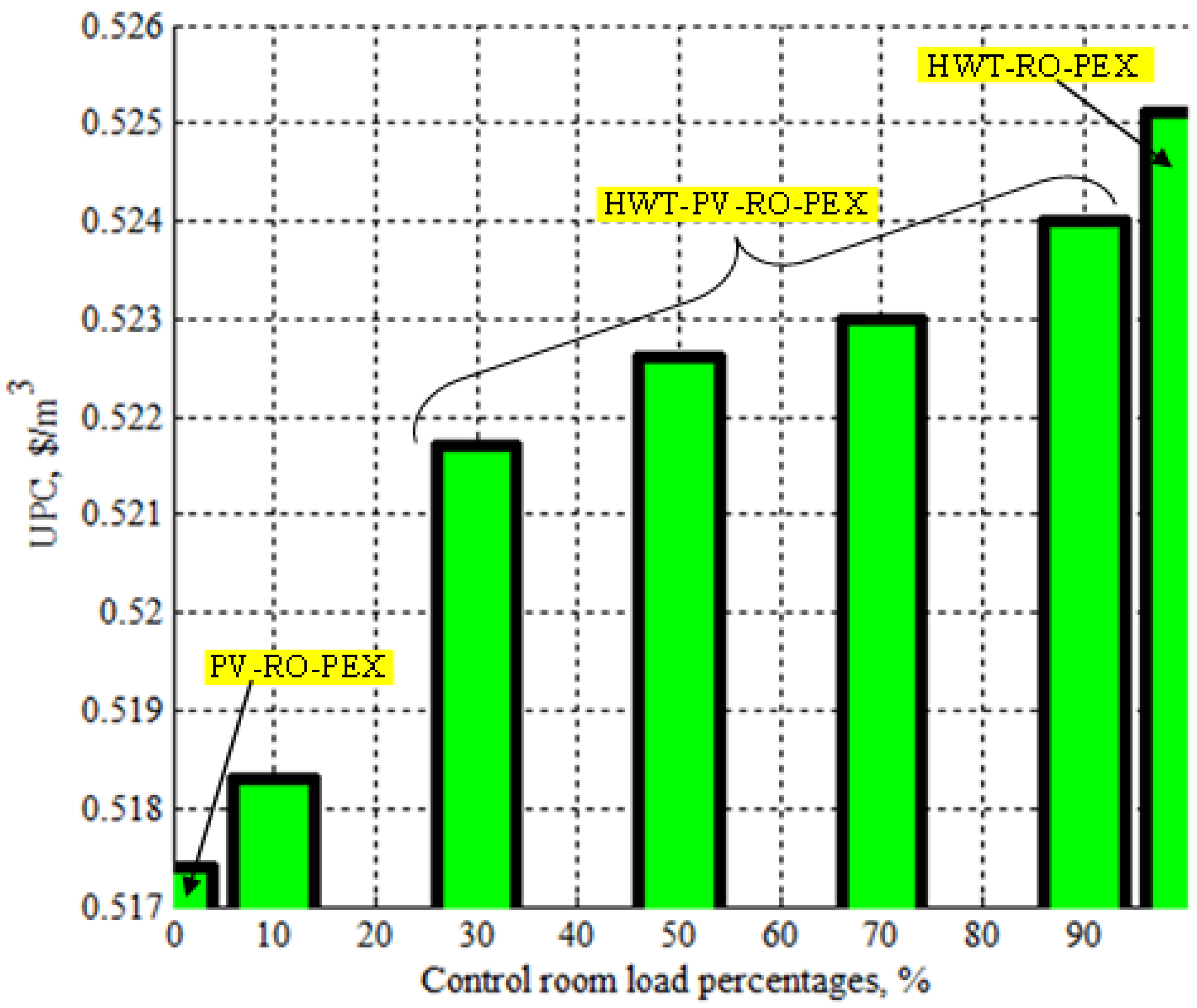
Maintaining less than a 5% load on the HWT farm to minimize UPC. For both operations, increasing the load percentage meant increasing the dependent load on the farm, and this work confirmed that was UPC is minimized when the load percentage was less than 5%; i.e., fully operational by the PV solar field. This operation gave a remarkable UPC of about 0.518 USD/m³.
Reducing the capital costs of PV panels to reduce the UPC so that it can compete with thermal systems. In a comparison with S-ORC-RO, the UPC of the PV-RO system was lower than that of the CSP-RO system; however, it may increase if the operation generates power over 10 MWe.

Generally, the CSP was favorable for larger categories of power generation up to 600 MW. The PV-RO and HWT-RO were proven promising for producing sustainable fresh water. PV-RO can compete against the HWT-RO or the S-ORC-RO for lower rates of fresh water production. HWT-RO and S-ORC-RO consume larger areas; however, they could be used for higher rates of power and fresh water production.

6. Recommendations

A wide range of varied operating conditions should be examined, and system performance should be studied using more design parameter variation.

Author Contributions

Methodology: A.M.S. and M.A.S.E.; formal analysis: A.M.S. and M.A.S.E.; software, M.A.S.E.; validation, A.M.S., A.G.A. and M.A.S.E.; formal analysis, A.M.S. and M.A.S.E.; investigation, A.M.S., A.G.A. and M.A.S.E.; resources, A.G.A.; administration, A.M.S.; funding acquisition, A.G.A.; writing—original draft preparation: A.M.S. and M.A.S.E.; review and editing: A.M.S. and A.G.A.; supervision: A.M.S.; project administration: A.G.A. All authors have read and agreed to the published version of the manuscript.

Funding

This work is supported by Ministry of Education in Saudi Arabia for funding this work through the project number 375213500.

Institutional Review Board Statement

Not applicable.

Informed Consent Statement

Not applicable.

Data Availability Statement

Not applicable.

Acknowledgments

The authors extend their appreciation to the Deputyship for Research & Innovation, Ministry of Education in Saudi Arabia for funding this work through the project number 375213500.

Conflicts of Interest

Authors declare no conflict of interest.

Nomenclature

A	Area: m²
Ac	Cell area, m²
Ae	Element area, m²
AH	Battery capacity, Ah
Am	Module area, m²
Ar	Rotor swept area m²
At	Total area, m²
BS	Battery storage, Wh
Cb	Battery cost, USD
Ct	Total cost, USD
CP	Turbine power coefficent
DCC	Direct capital cost, USD
DOD	Depth of discharge
Dr	Rotor diameter, m
FF	Fouling factor
FOBc	Full over board cost, USD
Gb	Solar flux, W/m²
HPP	High pressure pump
Hh	Hub height, m
HWT	Horizontal wind turbine
k	Permeability
M	Mass flow rate, m³/h, kg/s
n	Number, #
ne	Element number
NV	Number of pressure vessels
NOB	Number of batteries, #
NOC	Number of cells, #
NOM	Number of modules, #
NWT	Number of wind turbines, #
OH	Operating hours, h
P	Power, Permeator, or Pressure, bar
Pm	Module power, W
Pt	Total power, W
Pw	Wind power, kW
PV	Photovoltaic
ΔP	Pressure, bar
RR	Recovery ratio
RPMr	Rotor speed, rpm
SPC	Specific power consumption, kWh/m³
SR	Salt rejection
T	Temperature, °C
Tor	Torque, Nm
TCF	Temperature correction factor
UPC	Unit product cost, USD/m³
V	Volt
Vws	Start wind speed, m/s
Vwa	Average wind speed, m/s
X	Salinity, ppm
Subscripts
air	Ambient
b	Brine, battery
c	Cell
d	Distillate product
e	Element
f	Feed
m	Module
ORC	Organic rankine cycle
RO	Reverse osmosis
t	Turbine, total
v	Vessel
w	Water
Greek
η	Efficiency, %
Π	Osmotic pressure, kPa
ρ	Density, kg/m^r
ω	Rad/s

Appendix A

A: The RO Model

The mathematical model for the proposed RO unit is written as follows [2,24]:

The feed flow rate M_f based on recovery ratio RR and distillate flow rate M_d is

M_{f} = \frac{M_{d}}{R R}

(A1)

The distillate product salt concentration X_d is

X_{d} = X_{f} \times (1 - S R)

(A2)

where X_f is the feed flow rate salt concentration, and SR is the salt rejection percentage. The rejected brine is found from

M_{b} = M_{f} - M_{d}

(A3)

The rejected salt concentration kg/m³ is estimated by

X_{b} = \frac{M_{f} \times X_{f} - M_{d} \times X_{d}}{M_{b}}

(A4)

The average salt concentration kg/m³ is estimated as

X_{a v} = \frac{M_{f} \times X_{f} + M_{b} \times X_{b}}{M_{f} + M_{b}}

(A5)

The temperature correction factor TCF is found by

T C F = e x p (2700 \times (\frac{1}{273 + t} - \frac{1}{298}))

(A6)

Membrane water permeability k_W is

k_{w} = 6.84 \times 10^{- 8} \times (18.6865 - (0.177 \times X_{b})) / (t + 273))

(A7)

The salt permeability k_s is

k_{s} = F F \times T C F \times 4.72 \times 10^{- 7} \times (0.06201 - (5.31 \times 10^{- 5} \times (t + 273)))

(A8)

where FF is the membrane fouling factor. The calculations of osmotic pressure for the feed, brine, and distillate product are found as

Π_{f} = 75.84 \times X_{f}

(A9)

Π_{b} = 75.84 \times X_{b}

(A10)

Π_{d} = 75.84 \times X_{d}

(A11)

The average osmotic pressure on the feed side is

Π_{a v} = 0.5 \times (Π_{f} + Π_{b})

(A12)

The net osmotic pressure across the membrane is

Δ Π = Π_{a v} - Π_{d}

(A13)

The net pressure difference across the membrane is

Δ P = (\frac{M_{d}}{3600 \times T C F \times F F \times A_{e} \times n_{e} \times N_{v} \times k_{w}}) + Δ Π

(A14)

where A_e is the element area in m²; n_e is number of membrane elements; and N_v is the number of pressure vessels. The required power input in kW for the RO high pressure pump (HPP) is estimated as

H P P_{p o w e r} = \frac{1000 \times M_{f} \times Δ P}{3600 \times ρ_{f} \times η_{p}}

(A15)

where ρ_f is the feed flow rate density, and η_p is the driving pump mechanical efficiency. The specific power consumption in kWh/m³ is estimated as

S P C = \frac{H P P_{p o w e r}}{M_{d}}

(A16)

B: The HWT Model

The Horizontal Wind Turbine (HWT) as a part of wind desalination library (REDS [25]) was modeled according to the specification data obtained from the manufacture manual for many watt points, which vary from 0.5 to 8000 kW according to many companies. The data were obtained from more than 50 companies involved in wind turbine manufacturing. A developed model by Sharaf [26,27,28,29] was presented and correlated as a function of wind turbine power (P) as follows:

The starting wind speed m/s as a function of turbine power (kW):

V w_{s} = 13.37 \times ϵ^{({1.698}^{- 5} \times P)} - 10.72 \times ϵ^{(- 0.003214 \times P)}

(A17)

The average wind speed m/s:

V w_{a} = 9.378 \times (P^{0.09862})

(A18)

The rotor diameter m:

D r = 2.573 \times (P^{0.4414})

(A19)

The tower (Hub) height m:

H h = 1.437 \times (P^{0.5046}) + 5.354

(A20)

Air density kg/m³ is calculated based on air and pressure temperature:

ρ_{a i r} = \frac{P_{a i r} \times 100}{0.287 \times (T_{a i r} + 273.15)}

(A21)

where P_air is in bar and T_air is in °C.

The rotor swept area m² is then calculated based on the rotor diameter Dr:

A r = π \times {(D r / 2)}^{2}

(A22)

The air mass flow rate kg/s is then calculated based on the density, rotor swept area and average wind speed:

M_{a i r} = ρ_{a i r} \times A r \times V w_{a}

(A23)

The required wind power kW:

P_{w} = \frac{(\frac{1}{2} \times ρ_{a i r} \times A r \times (V w_{a}^{3})}{1000}

(A24)

The power coefficient is calculated from the assigned power P and the aerodynamic power Pw:

C P = \frac{P}{P_{w}}

(A25)

The rotor speed in rpm:

r p m_{r} = 347.6 \times (P^{- 0.2909}) - 16.91

(A26)

The rotor torque Tor in Nm based on the power of the turbine and the angular velocity (

ω

):

ω = \frac{(2 \times π \times R P M_{r})}{60}

(A27)

T o r = \frac{(1000 \times P)}{ω}

(A28)

The number of wind turbines can be calculated related to the total demanded power (TP kW) from the wind farm:

N W T = \frac{T P}{P}

(A29)

C: The PV Model

PV system was considered a very important power source in this work. It was modeled according to the actual data presented through more than 150 data points from the manufacturing manuals. The range of the operating modules type was from 5 to 280 W. Each module watt type can calculate the module specification based on the data fed in the table. Table A1 illustrates the inputs and outputs of the developed lookup table model block. SDS program [16,26] library is used to model and visualize the PV system program. The developed code is introduced to calculate the following:

Table A1. PV input and calculated parameters by the use of SDS program [25].

Inputs:

Outputs:

1—Operating hours (OH), h
2—Solar flux (G_b), W/m²
3—Number of cloudy days factor
4—System total power (P_t), kW
5—Module power (P_m) (5–280 W)
6—Battery depth of discharge (DOD)
7—Battery voltage (V_b), Volt
8—Battery efficiency, %
9—Battery unit price (C_b), USD

1—Open circuit voltage (V_oc), Volt
2—Short circuit current (I_sc), A
3—Maximum voltage (V_m), Volt
4—Maximum current (I_m), A
5—Cell and Module efficiencies, %
6—Net weight, kg
7—The dimensions, m²
8—Module price, USD/W
9—Number of cells and modules (NOC)
10—Cell area (A_c), cm²
11—Module area (A_m), m²
12—Total system area (A_t), m²
13—Battery storage, Wh
14—Battery capacity, Ah
15—Number of batteries (NOB)
16—Full over board cost (FOB_c), USD.

When calculating the main specifications (Table A1, parameters from 1 to 9) based on the module power, the following code was easily calculated. The number of modules (NOM) based on total power and module power:

N O M = \frac{P_{t}}{P_{m}}

(A30)

The module area in m² is then calculated based on module power P_m and efficiency

η_{m}

:

A_{m} = 100 \times \frac{P_{m}}{G_{b} \times η_{m}}

(A31)

Then the total area in m² was calculated:

A_{t} = A_{m} \times N O M

(A32)

The cell area in cm² based on the number of cells (NOC) that been calculated from the lookup table.

A_{c} = \frac{A_{m} \times 10^{3}}{N O C}

(A33)

The battery storage in Wh based on the operating hours (OH), number of cells (NOC), the total power (P_t), battery efficiency and depth of discharge (DOD):

B S = \frac{O H \times N O C \times P_{t}}{D O D \times η_{b}}

(A34)

If a 24 V system were chosen, the required (AH) of batteries would be 16,585/24,700.

A H = \frac{B S}{V_{m}}

(A35)

Number of batteries can be calculated as follows based on the maximum voltage and the battery voltage:

N O B = \frac{V_{m}}{V_{b}}

(A36)

The system total costs in (C_t, USD) are then calculated based on the full over board costs of the modules (FOB_c) and the batteries costs (C_b):

C_{t} = (P_{t} \times F O B_{c}) + (C_{b} \times N O B)

(A37)

where the FOB_c includes cables, connections, worker time, inverter unit, and maintenance costs.

D: Monthly average irradiation and wind speed

Figure A1. Monthly average irradiation for Suez Gulf region.

Figure A2. Monthly average wind velocity for Suez Gulf region.

References

Lamei, A.; van der Zaag, P.; von Münch, E. Basic cost equations to estimate unit production costs for RO desalination and long-distance piping to supply water to tourism-dominated arid coastal regions of Egypt. Desalination 2008, 225, 1–12. [Google Scholar] [CrossRef] [Green Version]
Nafey, A.; Sharaf, M. Combined solar organic Rankine cycle with reverse osmosis desalination process: Energy, exergy, and cost evaluations. Renew. Energy 2010, 35, 2571–2580. [Google Scholar] [CrossRef]
Mark, W.; Craig, B. Optimization of seawater RO systems design. Desalination 2005, 173, 1–12. [Google Scholar]
Qasim, M.; Badrelzaman, M.; Darwish, N.N.; Darwish, N.A.; Hilal, N. Reverse osmosis desalination: A state-of-the-art review. Desalination 2019, 459, 59–104. [Google Scholar] [CrossRef] [Green Version]
Mohamed, E.S.; Papadakis, G.; Mathioulakis, E.; Belessiotis, V. A direct coupled photovoltaic seawater reverse osmosis desalination system toward battery based systems—a technical and economical experimental comparative study. Desalination 2008, 221, 17–22. [Google Scholar] [CrossRef]
Helal, A.; Al-Malek, S.; Al-Katheeri, E. Economic feasibility of alternative designs of a PV-RO desalination unit for remote areas in the United Arab Emirates. Desalination 2008, 221, 1–16. [Google Scholar] [CrossRef]
Manolakos, D.; Mohamed, E.; Karagiannis, I.; Papadakis, G. Technical and economic comparison between PV-RO system and RO-Solar Rankine system. Case study: Thirasia island. Desalination 2008, 221, 37–46. [Google Scholar] [CrossRef]
Ahmad, G.; Schmid, J. Feasibility study of brackish water desalination in the Egyptian deserts and rural regions using PV systems. Energy Convers. Manag. 2002, 43, 2641–2649. [Google Scholar] [CrossRef]
Tzen, E.; Perrakis, K.; Baltas, P. Design of a stand alone PV-desalination system for rural areas. Desalination 1998, 119, 327–333. [Google Scholar] [CrossRef]
Liu, C.; Xia, W.; Park, J. A wind-driven reverse osmosis system for aquaculture wastewater reuse and nutrient recovery. Desalination 2007, 202, 24–30. [Google Scholar] [CrossRef]
de la Nuez Pestana, I.; Latorre, F.J.G.; Espinoza, C.A.; Gotor, A.G. Optimization of RO desalination systems powered by renewable energies. Part I Wind. Energy. Desalination 2004, 160, 293–299. [Google Scholar]
Dehmas, D.A.; Kherba, N.; Hacene, F.B.; Merzouk, N.K.; Merzouk, M.; Mahmoudi, H.; Goosen, M.F. On the use of wind energy to power reverse osmosis desalination plant: A case study from Ténès (Algeria). Renew. Sustain. Energy Rev. 2011, 15, 956–963. [Google Scholar] [CrossRef]
García-Rodríguez, L.; Romero-Ternero, V.; Camacho, C.G. Economic analysis of wind-powered desalination. Desalination 2001, 137, 259–265. [Google Scholar] [CrossRef]
Romero-Ternero, V.; García-Rodríguez, L.; Gómez-Camacho, C. Thermoeconomic analysis of wind powered seawater reverse osmosis desalination in the Canary Islands. Desalination 2005, 186, 291–298. [Google Scholar] [CrossRef]
Ma, Q.; Lu, H. Wind energy technologies integrated with desalination systems: Review and state-of-the-art. Desalination 2011, 277, 274–280. [Google Scholar] [CrossRef]
Dimitriou, E.; Boutikos, P.; Mohamed, E.S.; Koziel, S.; Papadakis, G. Theoretical performance prediction of a reverse osmosis desalination membrane element under variable operating conditions. Desalination 2017, 419, 70–78. [Google Scholar] [CrossRef]
Ruiz-García, A.; Nuez, I. Performance evaluation and boron rejection in a SWRO system under variable operating conditions. Comput. Chem. Eng. 2021, 153, 107441. [Google Scholar] [CrossRef]
Ruiz-García, A.; Nuez, I. Long-term intermittent operation of a full-scale BWRO desalination plant. Desalination 2020, 489, 114526. [Google Scholar] [CrossRef]
Nafey, A.S.; Sharaf, M.A.; García-Rodríguez, L. A new visual library for design and simulation of solar desalination systems (SDS). Desalination 2010, 259, 197–207. [Google Scholar] [CrossRef]
Delgado-Torres, A.M.; García-Rodríguez, L. Preliminary assessment of solar organic Rankine cycles for driving a desalination system. Desalination 2007, 216, 252–275. [Google Scholar] [CrossRef]
Nafey, A.; Sharaf, M.; Rodríguez, M.D.L.G. Thermo-economic analysis of a combined solar organic Rankine cycle-reverse osmosis desalination process with different energy recovery configurations. Desalination 2010, 261, 138–147. [Google Scholar] [CrossRef]
Sharaf, M.A.; Nafey, A.S.; García-Rodríguez, L. Exergy and thermo-economic analyses of a combined solar organic cycle with multi effect distillation (MED) desalination process. Desalination 2011, 272, 135–147. [Google Scholar] [CrossRef]
Toh, K.Y.; Lianga, Y.Y.; Lau, W.J.; Weihs, G.A.F. The techno-economic case for coupling advanced spacers to high-permeance RO membranes for desalination. Desalination 2020, 491, 114534. [Google Scholar] [CrossRef]
El-Dessouky, H.T.; Ettouney, H.M. Fundamental of Salt Water Desalination; Elsevier Science: Amsterdam, The Netherlands, 2002. [Google Scholar]
Eldean, M.A.S. Design and Simulation of Solar Desalination Systems. Ph.D. Thesis, Suez Canal University, Suez, Egypt, 2011. [Google Scholar]
Soliman, A.M.; Eldean, M.A.S.; Miraouia, I. Experimental and Economical Analysis of an Autonomous Renewable Power Supply System for Water Desalination and Electric Generation. Mod. Appl. Sci. 2019, 13, 43–64. [Google Scholar] [CrossRef] [Green Version]
Soliman, A.M.; Al-Falahi, A.; Mohamed AEldean, S.; Elmnifi, M. A new system design of using solar dish-hydro combined with reverse osmosis for sewage water treatment: Case study Al-Marj, Libya. Desalination Water Treat. 2020, 193, 189–211. [Google Scholar] [CrossRef]
Eldean, M.A.S.; El Shahat, A.; Soliman, A.M. A new modeling technique based on performance data for photovoltaic modules and horizontal axis wind turbines. Wind. Eng. 2017, 209–229. [Google Scholar]
Ansari, M.; Mudhar, A.; Obaidi, A.; Hadadian, Z.; Moradi, M.; Haghighi, A.; Mujtaba, I.M. Performance evaluation of a brackish water reverse osmosis pilot-plant desalination process under different operating conditions: Experimental study. Clean. Eng. Technol. 2021, 4, 100134. [Google Scholar] [CrossRef]

Figure 1. The proposed system model browser of the PV–HWT–RO using the SDS program. The system contains: 1, HWT; PV system; 3, control room unit; 4, RO desalination plant block.

Figure 2. Solar ORC model under SimuLink software browser by the use of SDS program: PTC, field, BHX unit, pumps, turbine unit, heat exchanger recuperator and RO plant block.

Figure 3. (a) Effect of feed splitter ratio and RO-PEX productivity on the UPC, USD/m³; (b) effect of feed/splitter ratio and no. of HWTs on the UPC, USD/m³.

Figure 4. (a) UPC, USD/m³ vs. PV power, W and RO–PEX feed splitter ratio, (b) UPC, USD/m³ vs. productivity, m³/day and RO–PEX feed splitter ratio (PV solar field without HWT farm).

Figure 5. The effect of control room load distribution and the UPC, USD/m³ (PV = 35 We module and HWT No. = 1 turbine).

Figure 6. Effect of HPP pressure and system productivity on (a) No. of pressure vessels, and (b) UPC in USD/m³.

Figure 7. Data comparison between PV-RO and S-ORC-RO: (a) area comparison, (b) UPC comparison.

Figure 8. The effect of HPP power, kWe on the solar filed area for both techniques thermal and electrical.

Figure 9. Comparison of UPC between Toh et al. [23] and the present work with different feed pressures.

Table 1. The specified parameters based on the design technique of modeling concept.

RO Model
Specified	Calculated
Fresh water productivity, m³/day	Feed and brine mass flow rates, kg/s
Seawater temperature, °C	Pressure on the HPP, bar
Seawater salinity, ppm	Average pressure, bar
HPP efficiency, %	Product and brine salinities, ppm
Booster pump efficiency, %	Salt rejection percentage, %
Membrane fouling factor, %	HPP power, kW
Number of elements/number of pressure vessels	SPC, kWh/m³
Element area, m²	Membrane area, m²
Recovery ratio, %
Pressure exchanger (PEX) efficiency, %
HWT Model
Specified	Calculated
Power/set, kW	Starting and average wind speeds, m/s, and air mass flow, kg/s
System total power, kW	Rotor diameter, m
Ambient temperature, °C	Hub height, m
Ambient pressure, bar	Rotor speed, rpm
	Swept area, m²
	Axial force, kN and Torque, kN
	Power coefficient, %
	Number of wind turbines
	Spacing between turbines in winddirection, m
	Spacing cross turbines in wind direction, m
	Total farm area, km²
PV Module
Specified	Calculated
Solar radiation, W/m²	The open circuit voltage, V and the short circuit current, A
Power/panel, W	The maximum voltage and current
Total system power, kW	The cell and module efficiencies, %
	The number of cells and modules of the system
	The module and system weights, kg, and areas, m²
	The battery bank capacity, A
S-ORC Model
Specified	Calculated
Solar radiation, W/m²	Solar Fields, condenser, recuperator areas, m²
Parabolic trough collector (PTC) high temperature, °C	Solar field dimensions and design
Boiler heat exchanger (BHX) effectiveness, %	Mass flow rates, kg/s
ORC turbine efficiency, %	ORC mass flow rates, kg/s
Recuperator effectiveness, %	Solar field mass flow rate, loop design, No. of collectors
Condensation temperature, °C	Heat rejected power, kW
Condenser effectiveness, %	PTC pump power, kW
	All thermo physical properties of all streams

Table 2. Preliminary data results for HWT–RO system for 3500 m³/day.

Environmental Conditions
Ambient temperature, °C	15 (winter)
Solar radiation, W/m²	350–400 (winter) [22]
Air pressure, bar	1.01
Seawater temperature, °C	20
RO Plant Results
Specific power consumption, kWh/m³	7.68
Power, kW	1131
Feed mass flow rate, m³/h	485.9
Production flow rate, m³/h	145.83
Brine flow rate, m³/h	340.1
Brine salinity, ppm	64180
Fresh water salinity, ppm	250
Salt rejection value	0.9944
RO high pressure, kPa	6850
HWT Farm Results
Total power for RO plant, kW	1131
Turbine power/wind power, kW	600/4762
Starting wind speed, m/s	4–11.95
Rated wind speed, m/s	17.62
Hub height, m	41.6
Rotor diameter, m	43.32
Swept area, m²	1474.08
Air mass flow rate, kg/s	3.173 × 10⁶
Torque (Nm)/rpm	1.542 × 10⁵/37.15
No. of wind turbines	2
Farm area, km²	0.06368
Cost Results
Plant life time/interest rate	25/5%
DCC of wind turbines, USD	1.174 × 10⁶
DCC of RO plant, USD	3.5 × 10⁶
Annual total costs, USD/year	6.31 × 10⁵
Unit product costs, USD/m³	0.5541

Table 3. Preliminary data results for PV–RO system for 3500 m³/day.

Environmental Conditions
The environmental conditions	Presented in Table 2
RO Plant Results
The RO results	Presented in Table 2
PV Site Results
Open circuit voltage/short circuit current, V/A	58.6/8.49
Maximum voltage/maximum current, V/A	47.4/4.641
Module efficiency/cell efficiency, %/%	15.45/17.5
No. of cells per module/No. of total modules	96/5135
Module dimensions/width, m³/mm	0.095/45
Net weight, kg	21.5
Cell area/module area, cm²/m²	423.8/4.06
Total system area, km²	0.02089
Battery storage, Wh	3.766 × 10⁶
Battery capacities, Ah	7.945 × 10⁴
No. of batteries—12 volt system	4
Cost Results
Plant life time/interest rate	25/5%
DCC of PV, USD	7.912 × 10⁵
DCC of RO plant, USD	3.5 × 10⁶
Annual total costs, USD/year	6.099 × 10⁵
Unit product costs, USD/m³	0.5305

Table 4. Preliminary data results for HWT–PV-RO system for 3500 m³/day.

Environmental Conditions
The environmental conditions	Presented in Table 2
RO Plant Results
The RO results	Presented in Table 2
HWT Farm Results
Total power for RO plant, kW	1131
Turbine power/wind power, kW	100/596.2
Starting wind speed, m/s	5.6
Rated wind speed, m/s	14.77
Hub height, m	20.03
Rotor diameter, m	19.64
Swept area, m²	303.1
Air mass flow rate, kg/s	5467
Torque (Nm)/rpm	1.288 × 10⁴/74.14
No. of wind turbines	6
Farm area, km²	0.03924
PV Site Results
Open circuit voltage/short circuit current, V/A	58.6/8.49
Maximum voltage/maximum current, V/A	47.4/4.641
Module efficiency/cell efficiency, %/%	15.45/17.5
No. of cells per module/No. of total modules	96/5135
Module dimensions/width, m³/mm	0.095/45
Net weight, kg	21.5
Cell area/module area, cm²/m²	423.8/4.06
Total system area, km²	0.01045
Battery storage, Wh	1.88 × 10⁶
Battery capacities, Ah	3.97 × 10⁴
No. of batteries (12 volt system)	4
Cost Results
Plant life time/interest rate	25/5%
DCC of HWT, USD	1.1 × 10⁶
DCC of PV, USD	3.958 × 10⁵
DCC of RO plant, USD	3.5 × 10⁶
Annual total costs, USD/year	6.604 × 10⁵
Unit product costs, USD/m³	0.5744

Table 5. Results comparison for different energy recovery devices.

Parameter:	Power, kW	SPC, kWh/m³	RO ΔP, bar	Power Reduction, %
Basic	1131	7.7	68.66	--
Stages = 9	917.47	6.3	35.8	18–20%
PEX	380–394	2.704	68.74	60–65%

Table 6. CSP vs. PV solar power generation.

Parameter	CSP (Thermal)	PV (Electric)
Resource quality	2400 kWh/m²/year	2445 kWh/m²/year
Power type	Thermal (indirect)	Electrical (direct)
Desalination system to combine with	All types (MSF, MED, MED–TVC, MED-MVC, RO, ED	RO, MED-MVC
Levelised cost of energy USD/MWh	60–350 (USD 214 in 2030)	100–450 (USD 303 in 2030)
Construction period/life time	2/30 years	1/30 years
Capacity factor	23–50%	20%
Power production	600 MW	10 MW
Heat engines	Stirling, Rankine, gas turbines, steam turbines	N/A

Publisher’s Note: MDPI stays neutral with regard to jurisdictional claims in published maps and institutional affiliations.

© 2021 by the authors. Licensee MDPI, Basel, Switzerland. This article is an open access article distributed under the terms and conditions of the Creative Commons Attribution (CC BY) license (https://creativecommons.org/licenses/by/4.0/).

Share and Cite

MDPI and ACS Style

Soliman, A.M.; Alharbi, A.G.; Sharaf Eldean, M.A. Techno-Economic Optimization of a Solar–Wind Hybrid System to Power a Large-Scale Reverse Osmosis Desalination Plant. Sustainability 2021, 13, 11508. https://doi.org/10.3390/su132011508

AMA Style

Soliman AM, Alharbi AG, Sharaf Eldean MA. Techno-Economic Optimization of a Solar–Wind Hybrid System to Power a Large-Scale Reverse Osmosis Desalination Plant. Sustainability. 2021; 13(20):11508. https://doi.org/10.3390/su132011508

Chicago/Turabian Style

Soliman, A. M., Abdullah G. Alharbi, and Mohamed A. Sharaf Eldean. 2021. "Techno-Economic Optimization of a Solar–Wind Hybrid System to Power a Large-Scale Reverse Osmosis Desalination Plant" Sustainability 13, no. 20: 11508. https://doi.org/10.3390/su132011508

Note that from the first issue of 2016, this journal uses article numbers instead of page numbers. See further details here.

Article Menu

Techno-Economic Optimization of a Solar–Wind Hybrid System to Power a Large-Scale Reverse Osmosis Desalination Plant

Abstract

1. Introduction

2. The Process Configurations

3. Simulation Methodology

4. Results and Comments

4.1. Non-Optimization Comparison Results

4.2. Comparison Results Based on Optimization

4.2.1. Technical Optimization Results

4.2.2. The Analytical Optimization Results

4.3. Data Results Compared with Solar-ORC

5. Conclusions

6. Recommendations

Author Contributions

Funding

Institutional Review Board Statement

Informed Consent Statement

Data Availability Statement

Acknowledgments

Conflicts of Interest

Nomenclature

Appendix A

References

Share and Cite

Article Metrics

Article Access Statistics

Further Information

Guidelines

MDPI Initiatives

Follow MDPI