
The Impact of Transformation of Farmers’ Livelihood on the Increasing Labor Costs of Grain Plantation in China

Abstract
:1. Introduction
2. Materials and Methods
2.1. Measurement of Labor Cost of Grain Production and Farmers’ Livelihood Transformation
2.2. Evaluation of Farmers’ Livelihood Transformation
2.3. Multiple Linear Regression Model of Farmers’ Livelihood Transformation and Labor Cost in Grain Production
3. Results
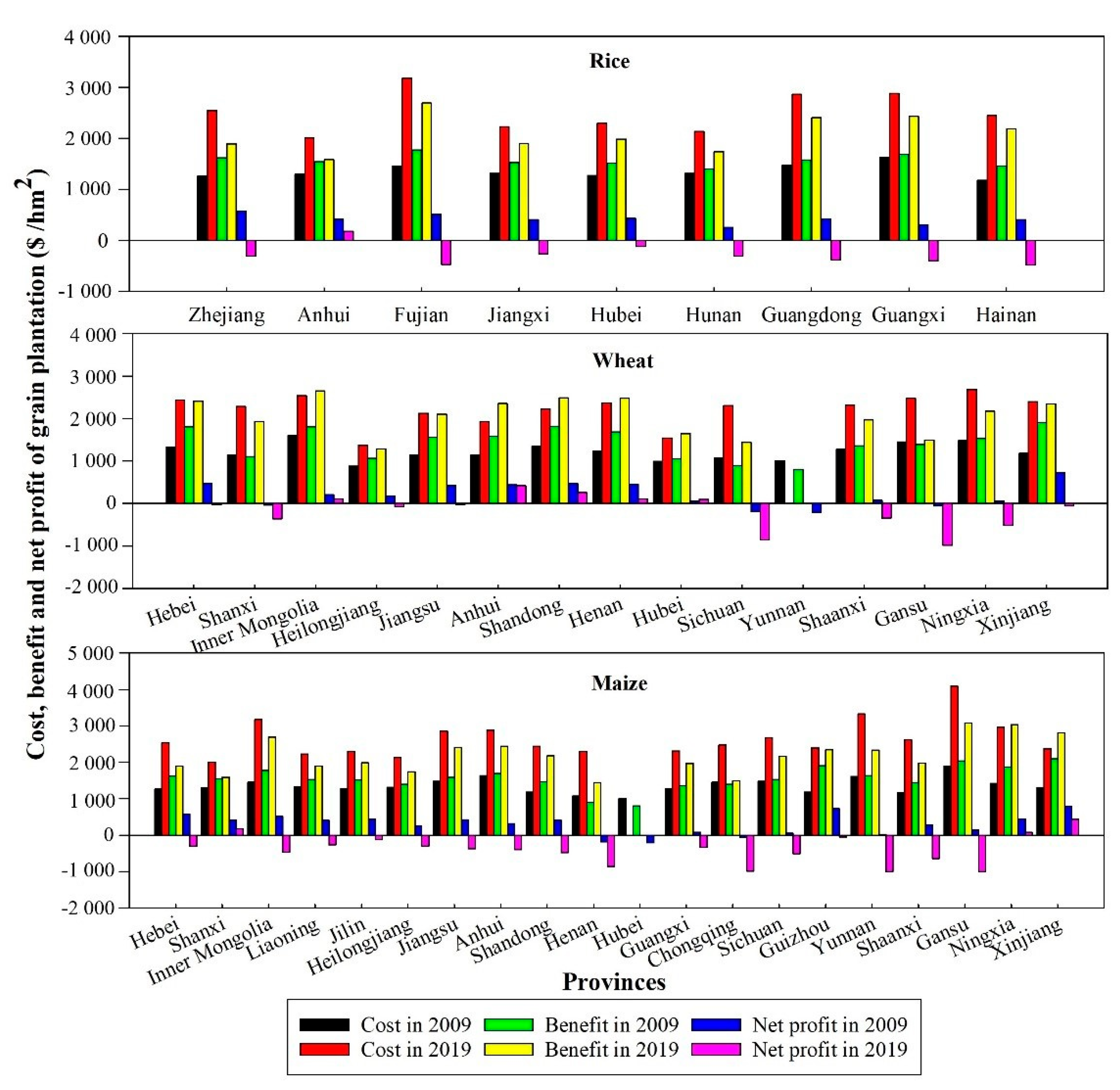
3.1. The Soaring Labor Cost in Grain Production
3.2. The Spatiotemporal Change in Farmers’ Livelihood Transformation
3.3. The Impact of Farmers’ Livelihood Transformation on the Labor Cost of Grain Production
4. Discussion
4.1. “Traps” Hidden in the Farmers’ Livelihood Transformation
4.2. Consequences of Soaring Labor Cost in Grain Production
4.3. Policy Implications
5. Conclusions
Author Contributions
Funding
Institutional Review Board Statement
Informed Consent Statement
Data Availability Statement
Acknowledgments
Conflicts of Interest
References
- Zhou, Y.; Li, X.; Liu, Y. Cultivated land protection and rational use in China. Land Use Policy 2021, 106, 105454. [Google Scholar] [CrossRef]
- The Price Department of National Development and Reform Commission of China. The Compilation of Cost-Benefit Data of National Agricultural Products (2009–2019); China Statistics Press: Beijing, China, 2020. Available online: https://data.cnki.net/Trade/yearbook/single/N2019010190?z=Z009 (accessed on 24 August 2020).
- Shi, B. Study on the Cost and Benefit of Grain Crop Production in Xinjiang—Take Wheat as an Example; Xinjiang Agricultural University: Ürümqi, China, 2018; pp. 1–59. [Google Scholar]
- Zhou, J.; Xie, Y.; Xiang, P. Emergy Analysis of Inputs and Outputs of Major Field Crop Ecosystems in Hunan Province. Crops 2021, 1, 175–181. (In Chinese) [Google Scholar] [CrossRef]
- Zhai, T.; Fan, Y.; Ma, G. Cost-benefit analysis and countermeasures of grain crops in Heilongjiang Province. Grain Sci. Technol. Econ. 2015, 1, 12–16. (In Chinese) [Google Scholar] [CrossRef]
- Yao, C.; Hou, F.; Chen, H. Logical relation and its policy implications between agricultural mechanization and food security: Based on a contrastive study of the cost and benefit of three main grain crops between China and the United States. J. Chin. Agric. Mech. 2021, 42, 1–8. (In Chinese) [Google Scholar] [CrossRef]
- Wang, G. The Dilemma of China’s Grain Production and the Choice of High-quality Development Path. J. China West Norm. Univ. 2021, 11–18. (In Chinese) [Google Scholar] [CrossRef]
- Huang, M.; Li, X.; Zeng, L. Impact of industrializaiton on rural labor price: Based on the test of the mediating effect of labor migration. J. China Agric. Univ. 2019, 24, 206–217. (In Chinese) [Google Scholar] [CrossRef]
- Yi, X.; Yan, Y. The impact of rural labor price fluctuation on grain production and its regional differences. J. South China Agric. Univ. 2019, 18, 70–83. (In Chinese) [Google Scholar] [CrossRef]
- Hu, X.; Zhong, F. The impact of rural population aging on food production: An analysis based on rural fixed observation data. Chin. Rural Econ. 2012, 6, 29–39. [Google Scholar]
- Wu, L.; Li, G.; Zhou, X. The demand and substitution relations of grain production factors. J. Zhongnan Univ. Econ. Law 2016, 2, 140–148. [Google Scholar]
- Mark, G.L. Adjusting the Herfindahl index for close substitutes: An application to pricing in civil aviation. Transport. Res. Part E. 2004, 40, 123–134. [Google Scholar] [CrossRef]
- Lee, S.; Chang, S.R.; Suh, Y. Developing Concentration Index of Industrial and Occupational Accidents: The Case of European Countries. Saf. Health Work. 2020, 11, 266–274. [Google Scholar] [CrossRef]
- Froese, L.; Dian, J.; Gomez, A.; Batson, C.; Sainbhi, A.S.; Zeiler, F.A. Association Between Processed Electroencephalogram-Based Objectively Measured Depth of Sedation and Cerebrovascular Response: A Systematic Scoping Overview of the Human and Animal Literature. Front. Neurol. 2021, 12, 692207. [Google Scholar] [CrossRef]
- Richard, H. Visualising the scales of ethnic diversity in London using a multilevel entropy. Environ. Plan. A 2020, 52, 1239–1242. [Google Scholar] [CrossRef] [Green Version]
- Devi, N.; Prasher, R.S. Growth and Diversification of Mountain Agriculture: A Case Study of Himachal Pradesh. Econ. Aff. 2019, 64, 47–53. [Google Scholar] [CrossRef]
- Ekhosuehi, V.; Osagiede, A. The use of entropy index for gender inequality analysis. Glob. J. Math. Sci. 2011, 9, 25–30. [Google Scholar] [CrossRef] [Green Version]
- Simpson, E.H. Measurement of Diversity. Nature 1949, 163, 688. [Google Scholar] [CrossRef]
- Subburayalu, S.; Sydnor, T. Assessing street tree diversity in four Ohio communities using the weighted Simpson index. Landsc. Urban Plan. 2012, 106, 44–50. [Google Scholar] [CrossRef]
- Liu, S.; Zhu, L.M.L.; Jiang, W.C.; Qin, J.Z.; Lee, H.S. Research on the effects of soil petroleum pollution concentration on the diversity of natural plant communities along the coastline of Jiaozhou bay. Environ. Res. 2021, 197, 111127. [Google Scholar] [CrossRef]
- W, Y.; Li, X.; Lu, D.; Yan, J. Evaluating the impact of land fragmentation on the cost of agricultural operation in the southwest mountainous areas of China. Land Use Policy 2020, 99, 105099. [Google Scholar]
- Leng, C.X.; Ma, W.L.; Tang, J.J.; Zhu, Z.K. ICT adoption and income diversification among rural households in China. Appl. Econ. 2020, 33, 3614–3628. [Google Scholar] [CrossRef]
- Johny, J.; Wichmann, B.; Swallow, B.M. Characterizing Social Networks and Their Effects on Income Diversification in Rural Kerala, India. World Dev. 2017, 94, 375–392. [Google Scholar] [CrossRef]
- Wu, Z. The calculation method of surplus livelihood ratio under the view of income difference. Product. Res. 2019, 6, 32–36. (In Chinese) [Google Scholar] [CrossRef]
- Rozelle, S. Success and failure of reform: Insights from the transition of agriculture. J. Econ. Lit. 2004, 42, 404–456. [Google Scholar] [CrossRef] [Green Version]
- Han, X.; Qu, L.L. Research on Efficiency of Financial Supports in Agricultural Industrialization in China. J. Northeast Agricul. Uni. 2016, 23, 78–81. [Google Scholar] [CrossRef]
- Zhang, D.H.; Wang, H.Q.; Lou, S. Research on grain production efficiency in China’s main grain-producing areas from the perspective of grain subsidy. Environ. Tech. Innov. 2021, 22, 101530. [Google Scholar] [CrossRef]
- Zhang, J.; Mishra, A.K.; Zhu, P.; Li, X. Land rental market and agricultural labor productivity in rural China: A mediation analysis. World Dev. 2020, 135, 105089. [Google Scholar] [CrossRef]
- Qiu, T.; Shi, X.; He, Q.; Luo, B. The paradox of developing agricultural mechanization services in China: Supporting or kicking out smallholder farmers? China Econ. Rev. 2021, 69, 101680. [Google Scholar] [CrossRef]
- Lu, W.C.; Chen, N.L.; Qian, W.X. Modeling the effects of urbanization on grain production and consumption in China. J. Integr. Agric. 2017, 16, 1393–1405. [Google Scholar] [CrossRef] [Green Version]
- Liu, Y.; Li, Y. Revitalize the world’s countryside. Nature 2017, 548, 275–277. [Google Scholar] [CrossRef]
- Sørensen, J.F. The rural happiness paradox in developed countries. Soc. Sci. Res. 2021, 98, 102581. [Google Scholar] [CrossRef]
- Van der Ploeg, J.; Laurent, C.; Blondeau, F.; Bonnafous, P. Farm diversity, classification schemes and multifunctionality. J. Environ. Manag. 2009, 90, S124–S131. [Google Scholar] [CrossRef]
- Visser, M.A.; Mullooly, J.; Campos-Melchor, P. Diversifying, transforming, and last resorts: The utilization of community based youth serving organizations in the construction of livelihood strategies by disconnected youth in rural America. J. Rural. Stud. 2020, 80, 328–336. [Google Scholar] [CrossRef]
- Gautam, Y.; Andersen, P. Rural livelihood diversification and household well-being: Insights from Humla, Nepal. J. Rural. Stud. 2016, 44, 239–249. [Google Scholar] [CrossRef] [Green Version]
- Hediger, W.; Knickel, K. Multifunctionality and Sustainability of Agriculture and Rural Areas: A Welfare Economics Perspective. J. Environ. Policy Plan. 2009, 11, 291–313. [Google Scholar] [CrossRef]
- Cheng, M.; Zhang, S.; Pan, X. Does migration of rural labor affects the grain yield?—An empirical analysis based on panel data of main production district in China. Res. Econ. Manag. 2013, 10, 79–85. [Google Scholar] [CrossRef]
- Zheng, L. The Impacts of Labor Migration on Farm Households’ Agricultural Produciton: Emipirical Evidences from 4 Countries in Jiangxi Province. Ph.D. Thesis, Zhejiang University, Hangzhou, China, 2011. [Google Scholar]
- Nguyen, D.L.; Grote, U.; Nguyen, T.T. Migration, crop production and non-farm labor diversification in rural Vietnam. Econ. Anal. Policy 2019, 63, 175–187. [Google Scholar] [CrossRef]
- Tong, Y.; Shu, B.; Piotrowski, M. Migration, Livelihood Strategies, and Agricultural Outcomes: A Gender Study in Rural China. Rural. Sociol. 2019, 84, 591–621. [Google Scholar] [CrossRef]
- Liu, Q.; Shumway, C.R. Geographic aggregation and induced innovation in American agriculture. Appl. Econ. 2006, 38, 671–682. [Google Scholar] [CrossRef]
- Kuroda, Y. The Production Structure and Demand for Labor in Postwar Japanese Agriculture, 1952–1982. Am. J. Agric. Econ. 1987, 69, 328–337. [Google Scholar] [CrossRef]
- Zheng, X.; Xu, Z. Endowment restriction, factor substitution and induced technological innovation: A case research on the grain producing mechanization in China. China Econ. Q. 2016, 16, 45–66. (In Chinese) [Google Scholar] [CrossRef]
- Lu, W. Research on the Impact of Rural Labor Migration on China’s Grain Production. Ph.D. Thesis, Nanjing Agricultural University, Nanjing, China, 2016. [Google Scholar]
- Damon, A.L. Agricultural Land Use and Asset Accumulation in Migrant Households: The Case of El Salvador. J. Dev. Stud. 2010, 46, 162–189. [Google Scholar] [CrossRef]
- Li, M.; Wang, Z.; Zhang, G. The impact of migrant labor on rice production in China. Agro Food Ind. Hi-Tech. 2016, 27, 53–58. [Google Scholar]
- Hayami, Y.; Ruttan, V.W. Factor Prices and Technical Change in Agricultural Development: The United States and Japan, 1880–1960. J. Political Econ. 1969, 78, 1115–1141. [Google Scholar] [CrossRef]
- Binswanger, H.P. A Cost Function Approach to the Measurement of Elasticities of Factor Demand and Elasticities of Substitution. Am. J. Agric. Econ. 1973, 56, 377–386. [Google Scholar] [CrossRef]
- Yamauchi, F. Rising real wages, mechanization and growing advantage of large farms: Evidence from Indonesia. Food Policy 2016, 58, 62–69. [Google Scholar] [CrossRef] [Green Version]
- Li, T.; Yu, W.; Baležentis, T.; Zhu, J.; Ji, Y. Rural demographic change, rising wages and the restructuring of Chinese agriculture. China Agric. Econ. Rev. 2017, 9, 478–503. [Google Scholar] [CrossRef]
- Zhu, S.; Xu, X.; Ren, X.; Sun, T.; Oxley, L.; Rae, A.; Ma, H. Modeling technological bias and factor input behavior in China’s wheat production sector. Econ. Model 2016, 53, 245–253. [Google Scholar] [CrossRef]
- Tian, X.; Yi, F.; Yu, X. Rising cost of labor and transformations in grain production in China. China Agric. Econ. Rev. 2019, 12, 158–172. [Google Scholar] [CrossRef]
- Wang, Y.; Shi, L.; Zhang, H.; Sun, S. A data envelopment analysis of agricultural technical efficiency of Northwest Arid Areas in China. Front. Agric. Sci. Eng. 2017, 4, 195–207. [Google Scholar] [CrossRef]
- Yang, S.; Wang, H.; Tong, J.; Ma, J.; Zhang, F.; Wu, S. Technical Efficiency of China’s Agriculture and Output Elasticity of Factors Based on Water Resources Utilization. Water 2020, 12, 2691. [Google Scholar] [CrossRef]


| Types | Contents | Explanation |
|---|---|---|
| Production cost | Labor cost | The cost of labors (home labors and hiring labors) in the process of sowing, ploughing, and harvesting, etc. |
| Material input cost | The cost of material inputs, such as chemical fertilizers, pesticides, and seeds. | |
| Land cost | Land cost | The cost of farmers subcontracting other farmers’ arable land, or renting the motorized land of the collective economic organization (such as land fixtures such as ditches, and motorized wells) |
| Indicator | Explanation |
|---|---|
| Income (IK) | |
| Wage income (I1) | The farmers’ income by engaging in a variety of part-time and sporadic jobs to obtain remuneration and benefits |
| Agricultural operation income (I2) | The farmers’ income from the regular household production and management activities, which mainly refers to the income from the agricultural products on their arable land |
| Property income (I3) | The farmers’ income from family-owned property (bank deposits, securities) and real property (houses, cars, collectibles, etc.), such as the income of renting a house or renting land. |
| Transfer income (I4) | The remittances from family members who are living outside the rural area, the subsidies, the insurance payments, the relief fund, pensions, compensation income from land acquisition, financial subsidies, and other transfer income |
| Expenditure (EK) | |
| Food (E1) | Farmers’ expenditure on categories E1–E8 |
| Clothing (E2) | |
| Accommodation (E3) | |
| Home equipment and services (E4) | |
| Transport and Communications (E5) | |
| Cultural and educational entertainment supplies (E6) | |
| Health care (E7) | |
| Other goods and services (E8) | |
| Variables | Instruction of the Indicator | |
|---|---|---|
| Dependent Variable | Y | The ratio of labor cost in the total cost of grain production |
| Independent variable () | X1 | Farmers’ Residual Livelihood Ratio |
| X2 | Farmers’ Livelihood Simpson Index | |
| Control variable () | X3 | Contribution of the primary industry to local GDP |
| X4 | Proportion of primary industry employees in local employees | |
| X5 | Price index of agricultural means of production, which is used to relatively reflect the price changes of agricultural means of production, including small farm tools, feed, mechanized farm tools, chemical fertilizers, pesticides and pesticide machinery, and oil for agricultural machinery. | |
| X6 | The proportion of expenditure on agriculture, forestry, and water resources in the total local public budget | |
| X7 | Mechanization input on per unit local arable land area | |
| X8 | Effective irrigation area | |
| X9 | Grain yield per unit area | |
| X10 | Engel’s coefficient of local farmers (the proportion of the food expenditure in the total expenditure) | |
| X11 | Non-grain plantation degree (the ratio of plantation area between local grain crops to economy crops) | |
| X12 | Non-agricultural land use degree (the proportion of cultivated land in total administrative land area) | |
| X13 | Urbanization level (the proportion of urban population in the total population) | |
| X14 | Local per capita disposable income |
| Year | Yield | Price | Revenue | Total Cost | Net Profit | Profit/Cost |
|---|---|---|---|---|---|---|
| (kg/hm2) | ($/t) | ($/hm2) | ($/hm2) | ($/hm2) | (%) | |
| Rice | ||||||
| 2009 | 6937.2 | 287.0 | 1992.5 | 1485.3 | 546.2 | 36.8 |
| 2019 | 7342.8 | 400.1 | 2744.3 | 2699.9 | 44.4 | 1.7 |
| Increment rate (%) | 5.9 | 39.4 | 37.7 | 81.8 | −91.9 | −95.5 |
| Wheat | ||||||
| 2009 | 5671.2 | 268.2 | 1519.2 | 1232.8 | 327.2 | 26.5 |
| 2019 | 6802.2 | 324.7 | 2269.9 | 2237.1 | 32.8 | 1.5 |
| Increment rate (%) | 19.9 | 21.1 | 49.4 | 81.5 | −90.0 | −94.5 |
| Maize | ||||||
| 2009 | 6449.1 | 237.7 | 1533.2 | 1198.2 | 381.3 | 31.8 |
| 2019 | 7558.5 | 259.5 | 2019.6 | 2295.3 | −275.6 | −12.0 |
| Increment rate (%) | 17.2 | 9.2 | 31.7 | 91.6 | −172.3 | −137.7 |
| Variables | Rice | Wheat | Maize | |||
|---|---|---|---|---|---|---|
| Tolerance | VIF | Tolerance | VIF | Tolerance | VIF | |
| The farmers’ residual livelihood ratio (X1) | 0.159 | 6.308 | 0.124 | 8.084 | 0.124 | 8.084 |
| The farmers’ livelihood Simpson Index (X2) | 0.130 | 7.694 | 0.149 | 6.694 | 0.149 | 6.694 |
| Contribution of the primary industry to local GDP (X3) | 0.109 | 9.202 | 0.109 | 9.202 | 0.122 | 8.202 |
| Proportion of primary industry employees in local employees (X4) | 0.038 | 26.584 | 0.038 | 26.584 | 0.152 | 6.584 |
| Price index of agricultural means of production (X5) | 0.464 | 2.155 | 0.103 | 9.715 | 0.103 | 9.715 |
| The proportion of expenditure on agriculture, forestry, and water resources in the total local public budget (X6) | 0.058 | 17.113 | 0.058 | 17.113 | 0.037 | 27.113 |
| Mechanization input on per unit arable land area (X7) | 0.376 | 2.662 | 0.171 | 5.853 | 0.171 | 5.853 |
| Effective irrigation area (X8) | 0.035 | 28.363 | 0.108 | 9.301 | 0.108 | 9.301 |
| Grain yield per unit area (X9) | 0.238 | 4.210 | 0.103 | 9.751 | 0.068 | 14.751 |
| Engel’s coefficient of local farmers (X10) | 0.144 | 6.925 | 0.121 | 8.298 | 0.108 | 9.298 |
| Non-grain plantation degree (X11) | 0.105 | 9.479 | 0.038 | 26.325 | 0.038 | 26.325 |
| Non-agricultural land use degree (X12) | 0.048 | 20.831 | 0.048 | 20.831 | 0.102 | 9.831 |
| Urbanization level (X13) | 0.059 | 16.809 | 0.147 | 6.809 | 0.147 | 6.809 |
| Local per capita disposable income (X14) | 0.113 | 8.866 | 0.039 | 25.957 | 0.100 | 9.957 |
| Variables | Standard Regression Coefficient | |||
|---|---|---|---|---|
| Rice | Wheat | Maize | ||
| The farmers’ residual livelihood ratio (X1) | X1 | −0.186 * | −0.173 * | −0.241 * |
| The farmers’ livelihood Simpson Index (X2) | X2 | 0.803 * | 0.057 * | 0.1 * |
| Contribution of the primary industry to local GDP (X3) | X3 | −0.762 | −0.222 | −0.256 |
| Proportion of primary industry employees in local employees (X4) | X4 | - | - | −0.536 |
| Price index of agricultural means of production (X5) | X5 | −0.4 | −0.067 | −0.014 |
| The proportion of expenditure on agriculture, forestry, and water resources in the total local public budget (X6) | X6 | - | - | - |
| Mechanization input on per unit arable land area (X7) | X7 | −0.431 ** | −0.183 ** | −0.319 ** |
| Effective irrigation area (X8) | X8 | - | −0.254 | −0.269 |
| Grain yield per unit area (X9) | X9 | −0.458 * | −0.820 * | - |
| Engel’s coefficient of local farmers (X10) | X10 | 0.1 * | 0.069 * | 0.124 * |
| Non-grain plantation degree (X11) | X11 | −0.653 * | - | - |
| Non-agricultural land use degree (X12) | X12 | - | - | −0.014 * |
| Urbanization level (X13) | X13 | - | −0.441 | −0.113 |
| Local per capita disposable income (X14) | X14 | 0.08 | - | 0.212 |
| R2 | 1.00 | 1.00 | 0.813 | |
| a-R2 | 0.815 | 0.806 | 0.661 | |
| DW | 1.682 | 1.519 | 2.246 | |
| F | 3.705 | 2.890 | 2.43 | |
| sig | 0.001 | 0.005 | 0.02 | |
Publisher’s Note: MDPI stays neutral with regard to jurisdictional claims in published maps and institutional affiliations. |
© 2021 by the authors. Licensee MDPI, Basel, Switzerland. This article is an open access article distributed under the terms and conditions of the Creative Commons Attribution (CC BY) license (https://creativecommons.org/licenses/by/4.0/).
Share and Cite
Jiang, X.; Yin, G.; Lou, Y.; Xie, S.; Wei, W. The Impact of Transformation of Farmers’ Livelihood on the Increasing Labor Costs of Grain Plantation in China. Sustainability 2021, 13, 11637. https://doi.org/10.3390/su132111637
Jiang X, Yin G, Lou Y, Xie S, Wei W. The Impact of Transformation of Farmers’ Livelihood on the Increasing Labor Costs of Grain Plantation in China. Sustainability. 2021; 13(21):11637. https://doi.org/10.3390/su132111637
Chicago/Turabian StyleJiang, Xilong, Guanyi Yin, Yi Lou, Shuai Xie, and Wei Wei. 2021. "The Impact of Transformation of Farmers’ Livelihood on the Increasing Labor Costs of Grain Plantation in China" Sustainability 13, no. 21: 11637. https://doi.org/10.3390/su132111637
APA StyleJiang, X., Yin, G., Lou, Y., Xie, S., & Wei, W. (2021). The Impact of Transformation of Farmers’ Livelihood on the Increasing Labor Costs of Grain Plantation in China. Sustainability, 13(21), 11637. https://doi.org/10.3390/su132111637