Numerical Analysis of the Structural Resistance and Stability of Masonry Walls with an AAC Thermal Break Layer

Abstract

Since energy efficiency has become the main priority in the design of buildings, load-bearing walls in modern masonry constructions nowadays include thermal break elements at the floor–wall junction to mitigate thermal bridges. The structural stability of these bearing walls is consequently affected. In the present paper, a numerical study of the resistance and stability of such composite masonry walls, including AAC thermal break layers, is presented. A finite element mesoscopic model is successfully calibrated with respect to recent experimental results at small and medium scale, in terms of resistance and stiffness under vertical load with or without eccentricity. The model is then used to extend the numerical models to larger-scale masonry walls made of composite masonry, with the aim of investigating the consequences of thermal elements on global resistance and stability. The results confirm that the resistance of composite walls is governed by the masonry layer with the lowest resistance value, except for walls with very large slenderness and loaded eccentrically: composite walls with low slenderness or loaded by a vertical load with limited eccentricities are failing due to the crushing of the AAC layer, while the walls characterized by large slenderness ratios and loaded eccentrically tend to experience buckling failure in the main clay masonry layer.

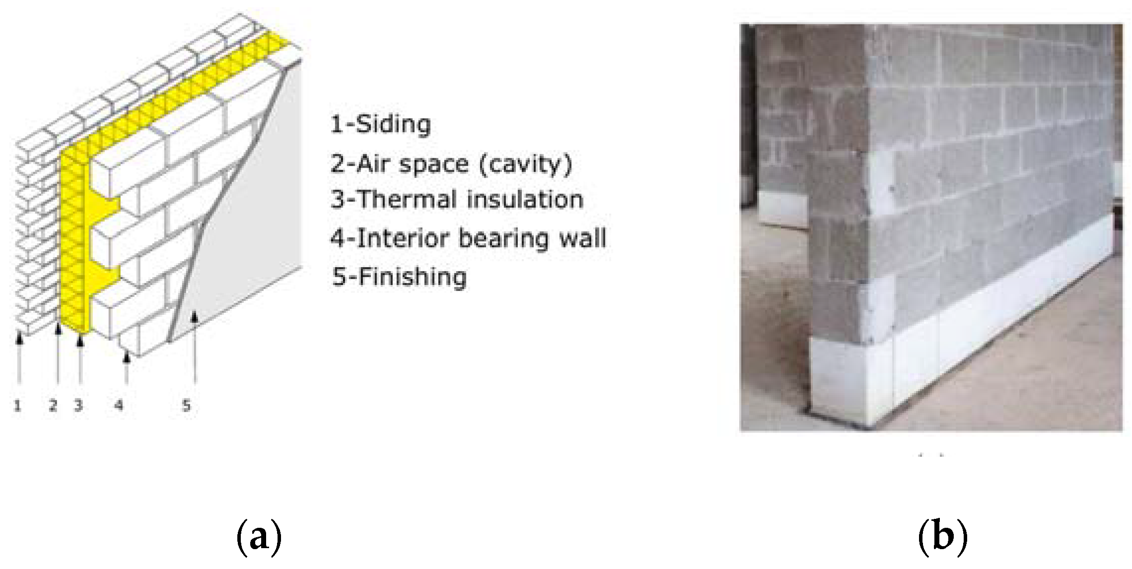
1. Introduction

The latest environmental concerns lead to significant changes in the construction of buildings, particularly for residential projects. Energy efficiency is now one of the main priorities in the conceptual design of a building. In order to improve the thermal performance of buildings, the heat losses are minimized through the integration of insulating layers. However, these materials affect the building structure as they may introduce mechanical discontinuities. In the particular case of masonry construction, the traditional monolithic wall has been replaced by a cavity wall consisting of several leaves (Figure 1a). In addition, more recently, thermal break elements have been introduced in, for instance, the inner leaf of such a cavity wall in order to eliminate thermal bridges and reduce the heat loss at several places around the buildings, particularly at the wall–floor junction, as shown in Figure 1b. In such a composite masonry wall, Aerated Autoclaved Concrete units (AAC), one of the most common thermal elements designed to replace the first layer of a load-bearing wall, are used in our study. AAC is a light building material made from lime, cement and sand [1,2,3] and is characterized by a low compressive strength up to 4.5 MPa [4].

Only a few studies have investigated the structural behavior of such composite masonry walls [7,8,9,10]. An experimental campaign by the authors [11] encompassed tests on small and medium-scale homogeneous and composite walls in order to understand their behavior and investigate the influence of the interaction between thermal and masonry elements on the local resistance. Results pointed out that the failure of composite specimens is always governed by the failure of the AAC material, which thus represents the weakest material. However, for larger composite walls, where buckling failure becomes more critical, there is a complete lack of experimental or numerical studies on how the presence of an AAC layer at the bottom would alter the boundary conditions and stiffness of the wall and consequently influence the buckling behavior. The available research results are essentially concerning the bearing resistance and stability of classical homogeneous masonry walls, i.e., built from one material [12,13,14,15,16,17,18,19,20]. The analytical solutions with regard to the stability of masonry walls and columns have been firstly investigated by Chapman and Slatford [21], Yokel [22], and Frish-Fay [23] based on equations for members under lateral deflection developed by Royen [24] and Angervo [25], assuming the members to behave linearly up to the failure, where tensile strength is not taken into account. Other studies [26,27,28,29,30,31,32,33,34] have improved the simulation of masonry behavior under critical load by including the material non-linearity, where it has been shown to better estimate the ultimate resistance and failure mechanism. Nonetheless, no literature is available on numerical studies concerning the behavior of large composite masonry walls.

In such a context, an extensive numerical study is conducted in this paper to explore the behavior of full-scale composite masonry walls incorporating a bottom layer consisting of AAC materials. The experimental tests on small-scale homogeneous and composite specimens, reported by the authors in [11] and summarized in Section 2.2, are used to calibrate the mechanical properties as performed in Section 3.1. Then, in Section 3.2, other selected tests from Sandoval et al. [18,19], on a different scale of homogeneous walls, are used to validate numerical models capable of capturing the stability behavior. The latter simulations are extended to composite wall models using the calibrated material input and combining other parameters (i.e., boundary conditions, stiffness). The numerical results in terms of average stress-lateral deformation curves and strain contour plots are used in Section 4 to assess the influence of thermal elements in combination with the other parameters on the stability and resistance of masonry walls at a global level. The finite element simulations are conducted using a mesoscopic approach using DIANA FEA [35], as described in Section 2.

2. Materials and Methods

Four stages of numerical simulations are carried out in this study, which is summarized in

Table 1. Overview of the models and their respective objectives.

Model Objective	Scale	Material Model	Constraints	Loading Conditions
Stage 1: Calibration of constitutive behavior and verification of the ability of the model to capture the experimental behavior (Section 3.1)	Medium-scale walls	Unit: total strain crack model; Interface: combined shear-tension-compression	Fixed at the bottom; partially fixed at the top	Centric compression
Stage 2: Verification of the ability of the model to capture the reduction in strength due to eccentricity using the experiments (Section 3.1)	Medium-scale walls	Unit: total strain crack model; Interface: combined shear-tension-compression	Fixed at the bottom; partially fixed at the top	Compression with eccentricity
Stage 3: Validation of the numerical model using Sandoval’s experiments [18] (Section 3.2)	Medium to large-scale walls	Unit: total strain crack model; Interface: combined shear-tension-compression	Pinned at both ends	Compression with eccentricity
Stage 4: Parametric study (Section 4)	Medium to large-scale walls	Unit: total strain crack model; Interface: combined shear-tension-compression	Pinned or fixed or partially fixed at both ends	Compression with or without eccentricity

. The first two stages are only considering the strength (or resistance) behavior, whereas the latter two stages are also considering instability (buckling) behavior. In the first stage, using a selection of experimentally tested homogeneous and composite wallets, as reported by the authors in [11] and summarized below, the constitutive model parameters are calibrated for centric (axial) loading conditions. In a second stage, these models are used in a validation study in which eccentric loading conditions are now considered, again using the aforementioned experiments. Then, in a third modeling stage, model validation is performed using the larger-scale eccentrically loaded wall tests executed by Sandoval et al. [18,19] in order to establish validated reference models capable of capturing the buckling behavior for multiple wall slendernesses. Finally, a parametric study is performed as a fourth modeling stage. It incorporates a set of medium and large-scale composite wall models with slenderness ratios ranging between 5 and 25, in combination with other parameters, i.e., load eccentricity, masonry stiffness, and boundary conditions. The latter models are built using, on the one hand, the calibrated material parameters obtained in the first two stages, and, on the other hand, the adapted numerical approach by means of loading conditions, analysis type, boundary conditions, and interface material model using the validated Sandoval models in the third stage.

The geometry of the simulated wallets and walls is represented in the height-thickness-plane, assuming the wall to behave uniformly on their length, in view of applying a physical eccentricity using a 2D “slice” model. This approach has been successfully used by other authors, such as Sandoval et al. [18,19], to capture the compressive strength reduction due to eccentricity.

2.1. Summary of the Experimental Tests and Corresponding Model Configurations

2.1.1. Experiments on Wallets by Deyazada et al.

In the experimental campaign on wallets, as reported by the authors in [11], both homogeneous AAC and composite AAC–clay specimens were tested under centric (e = 0) and eccentric compression (e = t/3 and e = t/6 with t the thickness of the wallet and e the distance between the applied load and the centerline of the wall). An overview of the tested specimens is presented in

Table 2. Overview of the tested specimens.

Specimen	Symbol	eP−R
Homogeneous AAC wallets with thin mortar layer under centric compression	W-HATLM	0
Composite AAC–clay wallets with thin mortar layer under centric compression	W-CCTLM	0
Homogeneous AAC wallets with thin mortar layer under eccentricity e = t/6	W-HATLM-et/6	t/6
Homogeneous AAC wallets with thin mortar layer under eccentricity e = t/3	W-HATLM-et/3	t/3
Composite AAC–clay wallets with thin mortar layer under eccentricity e = t/6	W-CCTLM-et/6	t/6
Composite AAC–clay wallets with thin mortar layer under eccentricity e = t/3	W-CCTLM-et/3	t/3

.

The corresponding model configuration as used in Section 3.1 is presented in Figure 2. As can be seen from the figure, the bottom nodes of the wallets are restrained in both horizontal and vertical directions, and the top nodes are only restrained in the horizontal direction. The vertical compressive loads are applied under displacement control at a rate of 0.1 mm per increment. For the finite element masonry models in this paper, a mesoscopic approach [36] is used, in which the masonry units are simulated using 16 × 16 2D plane stress isoperimetric continuum elements and mortar joints are modeled by zero-thickness interface elements. The material models of the units and joints are described in Section 2.2. The eccentricity of the reaction is controlled according to the real experiments by including a rigid plate at the bottom of the wall, with an adjustable width based on the amplitude of the desired eccentricity (see Figure 2b).

2.1.2. Buckling Experiments by Sandoval et al.

Sandoval and coworkers have conducted experimental tests and numerical simulations for a set of homogeneous clay walls under critical compressive loads in combination with different slenderness ratios and axial load eccentricities [18]. The walls were supported between two hinges at the top and the bottom, where they were placed in such a way that an eccentricity of the same magnitude was imposed at both ends of the wall. The walls had a variable height h whereas their lengths L = 300 mm and thickness t = 36 mm.

The modeling strategy used in Section 3.2 (i.e., material input, boundary conditions, analysis approach, mesh size) is similar to one of the numerical simulations performed by Sandoval [18]. The respective eccentricities and slendernesses of the benchmark models are presented in

Table 3. Benchmark models of homogeneous clay walls.

Model No.	Eccentricity	Slenderness
1	t/6	18.7
2	t/6	25.6
3	t/3	18.7
4	t/3	25.6

. The boundary conditions are simulated with a rigid triangle in which the end vertex varies to allow for different load eccentricities. The geometric non-linear behavior is taken into account to capture the stability behavior (using a total Lagrange definition of the strains). The non-linear material behavior of the masonry is, in this case, lumped into the bed mortar joints (see also Section 2.2), as failure usually occurs there for the current loading conditions, i.e., joint opening at the mid-height of the wall.

2.2. Material Models

The material model used to simulate the behavior of the masonry units is based on the total strain crack model proposed by Vecchio and Collins [37]. It has been used successfully by several authors [28,38,39] to describe the compressive and tensile behavior of the units, with stress-strain laws proposed for uniaxial compression and tension as presented in Figure 3. The compressive behavior of the units is represented by an equivalent parabolic stress-strain curve (Figure 3a) and the post-peak tensile behavior by an equivalent exponential stress-strain curve [4,30,32] (Figure 3b). This indicates that the model is essentially governed by crushing or cracking of the material.

The compressive behavior is governed by

$$f=\left\{\begin{array}{ll}-f_{\mathrm{c}}\frac{1}{3}\frac{k_j}{k_{\mathrm{c}/3}}& \mathrm{if} k_{\mathrm{c}/3}<k_{\mathrm{j}}\le 0\\ -f_{\mathrm{c}}\frac{1}{3}\left(1+4\left(\frac{k_{\mathrm{j}}-k_{\mathrm{c}/3}}{k_{\mathrm{c}}-k_{\mathrm{c}/3}}\right)-2{\left(\frac{k_{\mathrm{j}}-k_{\mathrm{c}/3}}{k_{\mathrm{c}}-k_{\mathrm{c}/3}}\right)}^2\right)& \mathrm{if} k_{\mathrm{c}}<k_{\mathrm{j}}\le k_{\mathrm{c}/3}\\ -f_{\mathrm{c}}\left(1-{\left(\frac{k_{\mathrm{j}}-k_{\mathrm{c}}}{k_{\mathrm{u}}-k_{\mathrm{c}}}\right)}^2\right)& \mathrm{if} k_{\mathrm{c}}<k_{\mathrm{j}}\le k_{\mathrm{u}}\\ 0& \mathrm{if} k_{\mathrm{j}}<k_{\mathrm{u}}\end{array}\right.$$

(1)

in which the material parameters

$$k_{\mathrm{c}/3}=-\frac{1}{3}\frac{f_{\mathrm{c}}}{E},$$

(2)

$$k_{\mathrm{c}}=-\frac{5}{3}\frac{k_{\mathrm{j}}}{k_{\mathrm{c}/3}}, \mathrm{and}$$

(3)

$$k_{\mathrm{u}}=k_{\mathrm{c}}-\frac{3}{2}\frac{G_{\mathrm{c}}}{h{f}_{\mathrm{c}}},$$

(4)

where $f_{\mathrm{c}}$ is the compressive strength; $k_{\mathrm{c}}$ is the strain at which the maximum compressive strength $f_{\mathrm{c}}$ is reached; $k_{\mathrm{u}}$ is the strain at which the material is entirely softened; $E$ is the Young’s modulus; $G_{\mathrm{c}}$ is fracture energy in compression; and $h$ is the crack band width, which is equal to $\sqrt{2A_{\mathrm{elem}}}$ for linear two-dimensional elements and $\sqrt{A_{\mathrm{elem}}}$ for higher-order two-dimensional elements [40]; A_elem is the area of the respective finite element. The tensile behavior of the bricks is, after the linear elastic phase, governed by

$$f=f_{\mathrm{t}}\exp \left[-\frac{h{f}_{\mathrm{t}}}{G_{\mathrm{fi}}}{K}_{\mathrm{t}}\right]$$

(5)

where $f_{\mathrm{t}}$ is the tensile strength; $G_{\mathrm{fi}}$ is the fracture energy in tension; $k_{\mathrm{t}}$ is the strain at which the material is entirely softened [36].

To model the mortar joints’ constitutive behavior, a combined interface model is used [36,39]. It is a rate-independent interface model based on a multi-surface plasticity model defined by a convex composite yield criterion, including a tension cut-off f₁(σ, κ₁), a Coulomb friction model f₂(σ, κ₂), and an elliptical compression cap f₃(σ, κ₃), as presented in Figure 4. This model is capable of modeling basic types of failure mechanisms that characterize masonry behavior, such as sliding along the mortar joints, cracking of the joints due to direct tension, combined shear, compression load, and masonry crushing, by means of splitting of units in tension due to mortar dilatancy at peak values of normal stress. For other interface aspects in masonry, including material determination and practical applications, the reader is referred to Lourenço, Rots and Van Zijl [36,41,42].

The tension cut-off mode $f_1\left(\sigma ,{\kappa }_1\right)={\overline{\sigma }}_1\left({\kappa }_1\right)$ is governed by an exponential softening regime expressed as

$${\overline{\sigma }}_1=f_{\mathrm{t}}\exp \left(-\frac{f_t}{{G_{\mathrm{f}}}^I}{\kappa }_1\right)$$

(6)

where $f_{\mathrm{t}}$ is the tensile strength of the masonry mortar; ${G_{\mathrm{f}}}^I$ is the mode I fracture energy; and ${\kappa }_1$ is the plastic relative displacement (i.e., jump).

The yield function of the Coulomb friction mode is expressed by

$$f_2\left(\sigma ,{\kappa }_2\right)=\left|\tau \right|+\sigma \tan \mathsf{\phi }\left({\kappa }_2\right)-{\overline{\sigma }}_2\left({\kappa }_2\right)$$

(7)

where

$${\overline{\sigma }}_2=c \exp \left(-\frac{c}{{G_{\mathrm{f}}}^{II}}{\kappa }_2\right)$$

(8)

in which $c$ is the cohesion of the unit–mortar interface, ${G_{\mathrm{f}}}^{II}$ is the mode II fracture energy, φ is the friction angle, and ${\kappa }_2$ is the shear plastic relative displacement. Finally, the yield function for the compression cap mode is governed by

$$f_3\left(\sigma ,{\kappa }_3\right)=c_{\mathrm{nn}}{\sigma }^2+c_{\mathrm{ss}}{\tau }^2+c_{\mathrm{n}}\sigma -{({\overline{\sigma }}_3\left({\kappa }_3\right))}^2$$

(9)

where $c_{\mathrm{nn}}$ and $c_{\mathrm{n}}$ are a set of material parameters to control the center of the cap and its intersection with the tensile part of the normal stress axis, $c_{\mathrm{nn}}$ is a material parameter that controls the contribution of the shear stress to failure, and ${\overline{\sigma }}_3$ is the yield value.

The material parameters used in the unit model are either extracted from experiments by the authors (discussed previously in [11]) through inverse numerical analysis of the compressive stress-strain curve, i.e., Young’s modulus $E$, compressive strength $f_{\mathrm{c}}$, fracture energy in compression $G_{\mathrm{fc}}$, or from relevant other recent experiments [3,43,44]. The material properties for the interface are either taken directly from the experiments presented in [11] or indirectly using data or formulas from the literature [4,18,37]. For example, the normal stiffness $k_{\mathrm{n}}$ and tangential stiffness $k_{\mathrm{s}}$ of the interface of the models are, respectively, calculated according to [36].

$$k_{\mathrm{n}}=\frac{E_{\mathrm{u}}{E}_{\mathrm{m}}}{h_{\mathrm{m}}\left(E_{\mathrm{u}}-E_{\mathrm{m}}\right)} \mathrm{and}$$

(10)

$$k_{\mathrm{s}}=\frac{G_{\mathrm{u}}{G}_{\mathrm{m}}}{h_{\mathrm{m}}\left(G_{\mathrm{u}}-G_{\mathrm{m}}\right)},$$

(11)

where $E_{\mathrm{u}}$ is the Young’s modulus of the masonry unit, $E_{\mathrm{m}}$ is the Young’s modulus of the mortar joint, $h_{\mathrm{m}}$ is the mortar thickness, $G_{\mathrm{u}}$ is the shear modulus the masonry unit, and $G_{\mathrm{m}}$ is the shear modulus of the masonry unit.

3. Numerical Simulations

3.1. Calibration and Validation of the Wallets’ Strength Using the Experiments by Deyazada et al.

The calibration starts with the modeling of homogeneous AAC wallets with a thin layer mortar. At the initial stage (simulation ‘Num1’ in

Table 4. Employed material parameters used throughout the numerical calibration process of a homogeneous AAC wallet model under centric compression. ‘Num15’ is the final, best-fitting parameter set (highlighted in grey).

Model	${\mathit{E}}_{\mathbf{y}}$	${\mathit{f}}_{\mathbf{c}}$	${\mathit{G}}_{\mathbf{f}\mathbf{c}}$
Num1	980	3.37	1.5
Num2	980	3.03	1.5
Num3	980	2.76	1.5
Num4	980	2.54	1.5
Num5	980	2.35	1.5
Num6	980	2.19	1.5
Num7	980	2.05	1.5
Num8	980	1.93	1.5
Num9	980	1.82	1.5
Num10	980	1.73	1.5
Num11	882	1.73	1.5
Num12	784	1.73	1.5
Num13	686	1.73	1.5
Num14	588	1.73	1.5
Num15	490	1.73	1.5
Num16	490	1.73	3.5
Num17	490	1.73	5

), material properties for the AAC units and the masonry interface are assumed based on relevant experimental data from literature [3,43,44]: the Young’s modulus $E_{\mathrm{y}}$ of the AAC unit is initially assumed to be 980 MPa, whereas the compressive strength $f_{\mathrm{c}}$ of the AAC unit has a starting value of 3.37 MPa. Next, the results of this simulation are compared with a selection of some representative individual specimens from the experiment conducted by Deyazada et al. [11] in terms of the stress-strain curves. An adjustment of the relevant material parameters is then carried out to obtain an agreement between the numerical and experimental results in terms of stiffness, ultimate strength, and softening of the stress-strain curve. For instance, it is found from the comparison between the experiments and the models with the initial values that the stiffness and ultimate compressive strength are overestimated because of the physical difference between the reality and the simplified 2D “slice” model (i.e., the model consists of four units on top of each other without considering the presence of head joints as in the test specimens). Therefore, to adapt the numerical model to the reality, the parameters affecting the stiffness and strength, namely $E_{\mathrm{y}}$ and $f_{\mathrm{c}}$, respectively, are varied until a satisfactory estimation is found. The fittest $E_{\mathrm{y}}$ and $f_{\mathrm{c}}$ values after calibration are 490 MPa and 1.73 MPa, respectively, i.e., 50% reduction on both parameters, see parameter set ‘Num15’ in Table 4.

After the selection of the most suitable material parameters on the basis of a limited sub-set of experimental results, the numerical model is validated against all specimens of the experiment conducted by Deyazada et al. [11]. The numerical validation of the homogeneous AAC wallet is presented in terms of average compressive stress-strain curves, as presented in Figure 5. The numerical results fall within the range of the experimental results in both elastic and inelastic stages up to the maximum load. The post-peak behavior is not perfectly captured due to limitations in the regularization and solver capabilities of the modeling software (DIANA FEA). However, these limitations have no influence on the obtained peak load: this was shown by a sensitive study, including masonry models with different meshes and convergence norms. Therefore, it can be concluded that the calibrated material inputs used to simulate the units and interface of homogeneous AAC wallets is satisfactory to predict the behavior of wallets under compression.

Next, simulations of AAC–clay composite wallets are executed. The material properties of the AAC units and interface are initially assumed identical to the final material parameters of the homogeneous AAC wallet (parameter set ‘Num1’ in

Table 5. Employed material parameters used throughout the numerical calibration process of a composite AAC–clay wallet model under centric compression. ‘Num6’ is the final, best-fitting parameter set (highlighted in grey).

Model	${\mathit{E}}_{\mathbf{y}}-\mathbf{AAC}$	${\mathit{E}}_{\mathbf{y}}-\mathbf{Clay}$	${\mathit{f}}_{\mathbf{c}}-\mathbf{AAC}$
Num1	490	2000	1.73
Num2	490	2000	1.87
Num3	490	2000	2.04
Num4	490	2000	2.21
Num5	490	2000	2.38
Num6	490	4000	2.38
Num7	490	6000	2.04
Num8	490	1000	2.04

). Material properties of clay units are extracted from experiments and literature. The effect of the head joints is managed in a similar way for the clay part of the wall, as previously described for the AAC layer, i.e., a reduction of 50% has also been applied on Young’s modulus and compressive strength of clay units, so $E_{\mathrm{y}}$ = 2000 MPa and $f_{\mathrm{c}}$ = 5 MPa. Then the results of this simulation are compared with the experimental results, and further calibration of the relevant material properties is performed to obtain an agreement between the numerical and experimental results, as can be seen in Figure 6. For example, from the comparison between the numerical and experimental results, it is noticed that the global compressive strength of the composite masonry should be increased to take into account the constraining effect of the clay units, which are stiffer and stronger, on the AAC units. Hence the compressive strength $f_{\mathrm{c}}$ of the AAC unit is adapted. The most suitable $f_{\mathrm{c}}$ value is found equal to 2.38 MPa, namely an increase with 40% (parameter set ‘Num6’ in Table 5).

After that, the numerical model with the calibrated material parameters is again validated against the full set of experimental results. The numerical validation of wallets is presented in terms of average compressive stress-strain curves. As it can be noticed from Figure 7, the numerical results of both wallets fall within the range of the experimental results in terms of the wall’s stiffness and resistance for the composite wallets up to the ultimate failure. Therefore, it can be concluded that the calibrated material parameters, as summarized in

Table 6. Calibrated material properties assumed for AAC and clay units used for modeling the units and wallets with and without eccentricity.

Parameter	Symbol	AAC	Clay	Unit
Young’s modulus	$E_{\mathrm{y}}$	490	4000	N/mm2
Poisson’s ratio	$v$	0.30	0.15	-
Compressive strength of unit (layer)	$f_{\mathrm{c}}$	1.73 (2.38) *	5	MPa
Fracture energy in compression	$G_{\mathrm{Fc}}$	1.50	5	Nmm/mm2
Tensile strength	$f_{\mathrm{t}}$	0.37	0.5	MPa
Fracture energy in tension	$G_{\mathrm{fi}}$	0.005	0.02	Nmm/mm2

* Values between brackets represent the compressive strength of the AAC units in composite walls.

and

Table 7. Material properties of the joint interface.

Interface Parameter	Symbol	Value	Unit
Normal stiffness AAC+AAC	$k_{\mathrm{n}}$	1000	N/mm3
Shear stiffness AAC+AAC	$k_{\mathrm{s}}$	400	N/mm3
Normal stiffness AAC+clay	$k_{\mathrm{n}}$	5000	N/mm3
Shear stiffness AAC+clay	$k_{\mathrm{s}}$	1000	N/mm3
Compressive strength	$f_{\mathrm{c}}$	20	MPa
Fracture energy in compression	$G_{\mathrm{fc}}$	15	Nmm/mm2
Tensile strength	$f_{\mathrm{t}}$	0.37	MPa
Fracture energy in tension	$G_{\mathrm{fi}}$	0.019	Nmm/mm2

, are reliable to predict the behavior of the units under compression, and therefore they could be used for the modeling of the larger masonry specimens in the subsequent sections.

The calibration process shows that the behavior of the masonry wall is mainly governed by the properties of the masonry units, where the interface parameters did not show any influence. This is because the AAC material is characterized with the lowest strength and stiffness (e.g., the mortar’s compressive strength >15 MPa whereas the AAC’s compressive strength <4 MPa).

Next, the models are extended, including homogeneous AAC and composite AAC–clay wallets subjected to three amplitudes of axial load eccentricities imposed from the bottom, as presented in Figure 2b. The accuracy of the wallet models under eccentricity is highlighted through a comparison between the numerical and experimental results in terms of the reduction in the failure load due to the eccentricity. On the other hand, the model has been compared with a simple theoretical reduction formula based on a rectangular stress block for homogeneous masonry, as adopted in EN 1996 [45,46].

The validation of the homogeneous and composite masonry models under eccentricity is depicted in Figure 8 in terms of strength reduction due to eccentricity (ratio of eccentric to concentric failure load). Numerical results show a logical trend, i.e., a reducing strength when increasing the eccentricity, for both homogeneous and composite wallets. However, there is a slight difference between the experimental and numerical results, in which the numerical results present more conservative values. For example, the numerical wallets exhibit a larger reduction in strength than the experimental ones, with a maximum difference of 24%. On the other hand, the comparison between the numerical results and the Eurocode formulation for both homogeneous and composite walls show that they are mostly in line with each other, illustrating a linear degradation of the bearing strength due to the application of the eccentricity. In other words, the models of the wallets under eccentricity seem sufficiently reliable to capture the reduction in strength due to eccentricity.

With regard to the failure mechanism, the predicted numerical failure agrees with the experimental observations for both homogeneous and composite wallets. For instance, the failure of the homogeneous AAC wallets with a non-centered base reaction is characterized by the initiation and development of vertical cracks firstly at the bottom from the end of the supported zone, then propagating towards the top of the wallet, as shown in Figure 9. In addition, the initiation and the development of cracks of the composite wallets are mainly observed in the supported zone of the bottom layer (Figure 10).

3.2. Validation of the Walls’ Strength and Stability Using the Experiments of Sandoval et al.

A geometrically non-linear model using the material parameters listed in

Table 8. Material properties of Sandoval’s model.

Parameter	Symbol	Value	Unit
Young’s modulus of units	$E_{\mathrm{y}}$	7500	N/mm2
Poisson’s ratio	$v$	0.15	-
Normal stiffness of the interface	$k_{\mathrm{n}}$	2380	N/mm3
Shear stiffness of the interface	$k_{\mathrm{s}}$	1035	N/mm3
Compressive strength masonry	$f_{\mathrm{c}}$	14.2	MPa
Fracture energy in compression	$G_{\mathrm{fc}}$	20.38	Nmm/mm2
Tensile strength	$f_{\mathrm{t}}$	0.55	MPa
Fracture energy in tension	$G_{\mathrm{fi}}$	0.008	Nmm/mm2

is subsequently validated against the work of Sandoval et al. [18] in terms of effective average stress-lateral deformation curves and failure mechanism, including out-of-plane stability behavior of the walls, see Figure 11. The average stress is defined as the maximum load divided by the total cross-sectional area of the wallets (i.e., L × t, t is the total thickness). The deformation parameter used in the curve represents the maximum lateral deflection in the wall at mid-height. The numerical model results indicate a good agreement with the experimental data. This includes the stress deformation curve and the collapse behavior, including horizontal joint opening at the wall mid-height. This means that the current model is capable of capturing the stability behavior and could be extended for simulating large composite walls, as conducted in Section 4.

4. Parametric Study

4.1. Parameters

The parameters listed in

Table 9. Case studies for homogeneous and composite masonry walls simulations (wall length L = 750 mm, wall thickness t = 150 mm, compressive strength of AAC unit f_c,AAC = 2.38 MPa, compressive strength of clay unit f_c,CL = 5 MPa, Young’s modulus $E_{\mathrm{y}}$ = 2000 MPa). $e$ refers to the eccentricity of the load.

No.	Model Name	Unit Combination	$\mathit{e}$	Slenderness Ratio/Wall Height (m)	B.C.
1	g-HA-e0-sl5	AAC+AAC	0	5/0.8	Pinned-pinned
2	g-HA-et6-sl5		t/6
3	g-HA-et3-sl5		t/3
4	g-HC-e0-sl5	Clay+clay	0	5/0.8	Pinned-pinned
5	g-HC-e0-sl15			15/2.2
6	g-HC-e0-sl21			21/3.2
7	g-HC-e0-sl26			26/4.0
8	g-HC-et6-sl5	Clay+clay	t/6	5/0.8	Pinned-pinned
9	g-HC-et6-sl15			15/2.2
10	g-HC-et6-sl21			21/3.2
11	g-HC-et6-sl26			26/4.0
12	g-HC-et3-sl5	Clay+clay	t/3	5/0.8	Pinned-pinned
13	g-HC-et3-sl15			15/2.2
14	g-HC-et3-sl21			21/3.2
15	g-HC-et3-sl26			26/4.0
16	g-CC-e0-sl5	AAC+clay	0	5/0.8	Pinned-pinned
17	g-CC-e0-sl15			15/2.2
18	g-CC-e0-sl21			21/3.2
19	g-CC-e0-SL26			26/3.2
20	g-CC-et6-sl5	AAC+clay	t/6	5/0.8	Pinned-pinned
21	g-CC-et6-sl15			15/2.2
22	g-CC-et6-sl21			21/3.2
23	g-CC-et6-sl26			26/4.0
24	g-CC-et3-sl5	AAC+clay	t/3	5/0.8	Pinned-pinned
25	g-CC-et3-sl15			15/2.2
26	g-CC-et3-sl21			21/3.2
27	g-CC-et3-sl26			26/4.0
28	g-CC-eg0-sl21-pp	AAC+clay	0	21/3.2	Pinned-pinned
29	g-CC-eg0-sl26-pp			26/4.0
30	g-CC-eg0-sl21-pfpf	AAC+clay	0	21/4.2	Partial fixed-partial fixed
31	g-CC-eg0-sl21-pfpf			26/5.4
32	g-CC-eg0-sl21-ff	AAC+clay	0	21/6.4	Fixed-fixed
33	g-CC-eg0-sl21-ff			26/8

and

Table 10. Case studies for homogeneous and composite masonry walls simulations (wall length L = 750 mm, wall thickness t = 150 mm, compressive strength of AAC unit f_C,AAC = 2.38 MPa, compressive strength of clay unit f_C,CL = 5 MPa, Young’s modulus $E_{\mathrm{y}}$ = 4000 MPa). $e$ refers to the eccentricity of the load.

No.	Model Name	Unit Combination	$\mathit{e}$	Slenderness Ratio/Wall Height (m)	B.C.
34	g-CC-e0-sl21	AAC+clay	0	21/3.2	Pinned-pinned
35	g-CC-e0-sl26			26/4.0
36	g-CC-et6-sl21	AAC+clay	t/6	15/2.2	Pinned-pinned
37	g-CC-et6-sl26			21/3.2
38	g-CC-eg0-sl21	AAC+clay	0	21/3.2	Pinned-pinned
39	g-CC-eg0-sl26			26/4.0

define the scope of the numerical parameter study. The considered parameters are as follows:

• Axial load eccentricity and slenderness

Three values of axial load eccentricities: e = 0, t/6 and t/3, combined with four levels of slenderness $h_{\mathrm{ef}}/t$ = 5, 15, 21 and 26, are considered. In the case of walls under centric loading conditions, a minimum eccentricity of 0.05t is applied in accordance with EN 1996 [47] to account for uncertainties on the load positioning, also useful in this numerical study to trigger the geometric non-linear response (similarly to the model developed by Sandoval et al.). The model scheme is presented in Figure 12.

• Geometrical imperfection, slenderness, and boundary conditions

The behavior of homogeneous and composite walls with geometrical imperfections $e_{\mathrm{g}}$ is investigated in combination with two levels of slenderness $h_{\mathrm{ef}}/t$ = 21 and 26 and three types of boundary conditions, namely pinned-pinned conditions, fixed-fixed conditions and semi-fixed conditions, as presented in Figure 12b–d. The geometrical imperfection $e_{\mathrm{g}}$ is accounting for a possible irregularity of the wall geometry. The imperfection has been applied by adjusting the geometry of the wall with a deviation at mid-height equal to $h_{\mathrm{ef}}/450$, as specified by EN 1996 [45,46]. The effective height $h_{\mathrm{ef}}$ is equal to ${\rho }_{\mathrm{n}}$ × $h$, where $h$ is the wall height, ${\rho }_{\mathrm{n}}$ equals to 1 for a pinned-pinned support, 0.75 for partially fixed support conditions at both ends, and 0.5 for a fixed-fixed support. The pinned supports are simulated with a rectangular rigid plate, restrained in the middle in the vertical and horizontal directions, as depicted in Figure 12b, whereas the fixed supports are simulated with a fully restrained rectangular rigid plate (Figure 12c). The partially fixed supports have been modeled resorting to rotational springs (Figure 12d). The stiffness of the springs is calibrated based on a linear stability analysis, in such a way that the Euler buckling load is equal to $P_{\mathrm{cr}}=\frac{{\pi }^{2}EI}{{\left({\rho }_{\mathrm{n}}L\right)}^2}$ with ${\rho }_{\mathrm{n}}=0.75$, where $P_{\mathrm{cr}}$ is the ultimate buckling load, $E$ is the Young’s modulus of wall, and $I$ is the moment of inertia.

• Masonry stiffness

The influence of a variation of the stiffness of the upper clay layers in composite walls is investigated. Two different values of the Young’s modulus $E_{\mathrm{y}}$ of the main clay masonry are assumed, namely 2000 and 4000 Mpa. Concerning the homogeneous masonry walls, design codes, including EN 1996 [45,46], and other studies [19,32,47,48,49,50,51,52,53,54] suggest a crucial relationship between the stiffness of the wall and the compressive strength of masonry walls, i.e., the ultimate strength increases when the stiffness of the wall increases.

• Homogeneous vs. composite specimens

A comparison between homogeneous and composite specimens with different material combinations is illustrated to determine whether the AAC or clay in a composite context behaves differently than when they are used separately in homogeneous walls. The simulated models encompass three types: homogeneous clay walls, composite AAC–clay walls and short homogeneous AAC walls (the slenderness of the AAC wall is kept the same with a ratio equal to five).

The material model for these models includes material non-linearity for both units and interfaces as the composite walls are expected to fail either by the crushing of the AAC material or due to the opening of the bed joint in the middle. This is different from Sandoval’s models (Section 3.2), where material non-linearity is only assumed in the interface since failure is mainly expected to occur there.

4.2. Results and Discussion

The resulting stress-deformation curves and failure patterns will be used to illustrate the influence of the different parameters. Effective stress is defined as the total load divided by the gross area of the wallets (i.e., L × t with t is the overall wall thickness) (Table 9 and Table 10).

• Slenderness and eccentricity

As it can be noticed in Figure 13, the homogeneous clay specimens experience a consistent strength reduction in the bearing resistance when the slenderness or the eccentricity increase. The composite walls exhibit a similar consistent reduction due to the increase of eccentricity, while the influence of the slenderness on the behavior of composite walls is only evidenced for the walls with large slenderness ratios, i.e., $h_{\mathrm{ef}}/t$ = 21 and 26. The reason is that when composite walls have low slenderness, the failure will occur through a local failure of the AAC layer, for which the global slenderness does not play any role. In addition, there is a consistent increase in the lateral deformation at the failure of the composite walls when the level of slenderness is increased (see Figure 13d–f).

• Boundary conditions

A comparison between walls with the same slenderness, eccentricity and material parameters but with different boundary conditions is illustrated in terms of resistance and failure behavior. The aim is to investigate the influence of modifying the boundary conditions on the behavior of composite walls. As it can be noticed in

Table 11. Results for the masonry walls with different boundary conditions in terms of vertical stresses.

Specimen	Stress (MPa)	Failure Mode
g-CC-eg0-sl21-pp	2.10	Strength failure of AAC layer
g-CC-eg0-sl21-pfpf	2.19	Strength failure of AAC layer
g-CC-eg0-sl21-ff	1.88	Strength failure of AAC layer
g-CC-eg0-sl26-pp	1.49	Stability failure of main clay masonry
g-CC-eg0-sl26-pfpf	1.61	Strength failure of AAC layer
g-CC-eg0-sl26-ff	1.08	Strength failure of AAC layer

, the resistance and failure behavior of composite walls is indeed influenced by a modification of the boundary conditions. The failure behavior of the very slender wall (i.e., the slenderness ratio equals 26) with pinned-pinned conditions experienced stability failure, while the walls with other boundary conditions experienced material failure in the AAC layer, leading to lower resistance for the walls with fixed-fixed boundary conditions. The reason for that is related to the bending moment distribution in the wall. The moment for walls with fixed boundary conditions is larger at the level where AAC units are present, in contrast to a wall with pinned-pinned conditions, where the maximum moment is expected to be at the mid-height of the wall.

• Masonry stiffness

The influence of a varying Young’s modulus of the clay units on the resistance and stability of composite masonry walls is illustrated in

Table 12. Results for the masonry walls with different masonry stiffness in terms of vertical stresses. Group 1: f_c = 5 MPa, E_y = 2000 MPa; Group 2: f_c = 5 MPa, E_y = 4000 MPa.

Specimen	Stress (Group 1) (MPa)	Failure Mode	Stress (Group 2) (MPa)	Failure Mode
g-CC-e0-sl21	1.98	Material failure of AAC layer	2.06	Material failure of AAC layer
g-CC-e0-sl26	1.53	Stability failure of main clay masonry	1.95	Material failure of AAC layer
g-CC-et6-sl21	1.12	Stability failure of main clay masonry	1.30	Material failure of AAC layer
g-CC-et6-sl26	0.82	Stability failure of main clay masonry	1.28	Stability failure of main clay masonry
g-CC-eg0-sl21-pp	2.10	Material failure of AAC layer	2.23	Material failure of AAC layer
g-CC-eg0-sl26-pp	1.49	Stability failure of main clay masonry	2.20	Material failure of AAC layer

. The results show that increasing the stiffness of the clay units generally leads to an increase in the resistance of composite walls and, in many cases, also affects the failure pattern. For example, the resistance of the composite wall g-CC-e0-sl26 increased from 1.53 to 1.95 MPa. The failure mode is shifting from stability failure in the clay part of the masonry to a material failure in the AAC units. In other cases, the resistance of composite wall g-CC-e0-sl21 increases slightly from 1.98 to 2.06 MPa, where the main failure occurs again in the AAC layer. This tends to agree with the stability formula in EN 1996 for homogeneous specimens, i.e., improving the stiffness of the unit has a positive effect on the ultimate compressive strength.

• Failure mechanism

The typical failure patterns of composite specimens are presented in

Table 13. Failure mechanism of the executed composite masonry models.

Specimen	Failure Mode
g-CC-e0-sl5	Material failure of AAC layer
g-CC-et6-sl5	Material failure of AAC layer
g-CC-et3-sl5	Material failure of AAC layer
g-CC-e0-sl15	Material failure of AAC layer
g-CC-et6-sl15	Material failure of AAC layer
g-CC-et3-sl15	Material failure of AAC layer
g-CC-e0-sl21	Material failure of AAC layer
g-CC-et6-sl21	Material failure of AAC layer
g-CC-et3-sl21	Stability failure of main clay masonry
g-CC-e0-sl26	Stability failure of main clay masonry
g-CC-et6-sl26	Stability failure of main clay masonry
g-CC-et3-sl26	Stability failure of main clay masonry

and displayed in Figure 14 and Figure 15 in terms of vertical strain contour plots. Two types of failure are observed according to the level of slenderness or eccentricity, as already mentioned above. One is characterized by the collapse of the AAC layer only. This failure is likely to happen for walls with small slenderness ratios and/or subjected to a low level of eccentricity (see Figure 14 for model g-CC-e0-sl21). The other type of failure is characterized by a stability failure of the clay masonry layers in the middle of the wall and is expected for walls with a higher slenderness ratio and/or characterized by a large loading eccentricity (see Figure 14 for g-cc-et3-sl26). For walls with a geometrical imperfection, whatever the boundary conditions, failure is governed by the collapse of the AAC layer except for model g-cc-eg0-pp, which exhibited stability failure (see Figure 15). In case of AAC material failure, a large lateral strain is experienced, particularly at the AAC layer. In case of stability failure, large strains are experienced at mid-height of the wall (where large lateral deflections are observed).

• Composite vs. homogeneous specimens

To improve the understanding of the structural behavior of a thermal layer and the main clay masonry in a composite wall and to investigate whether both components behave rather as two homogeneous walls above each other or really with a global composite behavior, the compressive resistance of both homogeneous and composite specimens is summarized in Figure 16. It appears that the thermal layer in a composite wall can be assumed as behaving as a short AAC wall (namely an AAC wall with a slenderness ratio h_ef/t < 6), while the clay part behaves as a homogeneous clay wall having its actual height, but whose resistance would be the resistance of the weakest layer. This is obvious, for instance, from a comparison between a composite wall with given eccentricity and limited slenderness, i.e., h_ef/t = 15, and a homogeneous AAC wallet with the same eccentricity. For example, both a homogeneous AAC wall with e = 0 and h_ef/t = 5 and a composite wall with e = 0 and h_ef/t = 15 experience crushing of the AAC units, with their resistance being equal to 1.66 and 2.30 MPa, respectively, while the resistance of a composite wall with e = t/3 and h_ef/t = 26 and the resistance of a homogeneous clay wall with e = t/3 and h_ef/t = 26 is for both cases equal to 0.36 MPa, with a failure due to instability.

5. Summary and Conclusions

Numerical models of a set of homogeneous AAC and composite AAC–clay wallets are calibrated against experimental results from the authors complemented by additional tests from literature in order to derive suitable material properties. The numerical models show a satisfactory prediction capacity of the experimental behavior in terms of ultimate strength and deformation behavior. The models are then used for a parametric study to assess the behavior of homogeneous and composite walls with various slenderness ratios, loading eccentricity, stiffness and boundary conditions and to evaluate their resistance and overall stability.

The results confirm that the resistance of composite walls is governed by the masonry layer with the lowest resistance value, except for walls with very large slenderness and loaded eccentrically: composite walls with low slenderness (up to a slenderness ratio of 15) or loaded by a vertical load with limited eccentricities are failing due to the crushing of the AAC layer, which is characterized by the lower strength, while the walls characterized by large slenderness ratios (e.g., $h_{\mathrm{ef}}/t$ ≥ 21) and loaded eccentrically tend to experience buckling failure in the main clay masonry layer.

The results show that using stiffer clay units considerably affects the resistance and failure mechanism of composite walls. The higher the stiffness of the clay unit, the better the stability behavior of the main clay masonry part of the wall and, consequently, of the global composite wall.

References

- Limbachiya, M.C.; Roberts, J.J. Autoclaved Aerated Concrete: Innovation and Development; Taylor & Francis: Abingdon-on-Thames, UK, 2005. [Google Scholar]
- Laukaitis, A.; Fiks, B. Acoustical properties of aerated autoclaved concrete. Appl. Acoust. 2006, 67, 284–296. [Google Scholar] [CrossRef]
- Ferretti, D.; Michelini, E.; Rosati, G. Cracking in autoclaved aerated concrete: Experimental investigation and XFEM modeling. Cem. Concr. Res. 2015, 67, 156–167. [Google Scholar] [CrossRef]
- Trunk, B.; Schober, G.; Helbling, A.K.; Wittmann, F.H. Fracture mechanics parameters of autoclaved aerated concrete. Cem. Concr. Res. 1999, 29, 855–859. [Google Scholar] [CrossRef]
- WTCB. Thermische Isolatie van Bestaande Muren; WTCB: Bruxelles, Belgium, 2016. [Google Scholar]
- Xella. Ytong Gehydrofobeerde Kimblok; Xella: Burcht, Belgium, 2016. [Google Scholar]
- Mordant, C.; Denoël, V.; Degée, H. Rocking behaviour of simple unreinforced load-bearing masonry walls including soundproofing rubber layers. In Proceedings of the 5th International Conference on Computational Methods in Structural Dynamics and Earthquake Engineering Methods (COMPDYN 2015), Crete, Greece, 25–27 May 2015. [Google Scholar]
- Mordant, C.; Dietz, M.S.; Taylor, C.A.; Plumier, A.; Degée, H. Seismic Behavior of Thin-Bed Layered Unreinforced Clay Masonry Shear Walls Including Soundproofing Elements. In Seismic Evaluation and Rehabilitation of Structures; Springer: New York, NY, USA, 2014; pp. 77–93. [Google Scholar]
- Deyazada, M.; Vandoren, B.; Degée, H. Experimental and numerical investigations on the influence of thermal elements on structural stability of masonry walls. In Proceedings of the 16th International Masonry Conference, Padova, Italy, 26–29 June 2016. [Google Scholar]
- Martens, D. Thermal Break with Cellular Glass Units in Load-Bearing Masonry Walls. In Proceedings of the 9th International Masonry Conference, Guimarães, Portugal, 7–9 July 2014. [Google Scholar]
- Deyazada, M.; Vandoren, B.; Degée, H. Experimental investigations on the resistance of masonry walls with AAC thermal break layer. Constr. Build. Mater. 2019, 224, 474–492. [Google Scholar] [CrossRef]
- Cavaleri, L.; Failla, A.; la Mendola, L.; Papia, M. Experimental and analytical response of masonry elements under eccentric vertical loads. Eng. Struct. 2005, 27, 1175–1184. [Google Scholar] [CrossRef]
- Tensing, D. Experimental study on axial compressive strength and elastic modulus of the clay and fly ash brick masonry. J. Civ. Eng. Constr. Technol. 2013, 4, 134–141. [Google Scholar]
- Colville, J. Stability of unreinforced masonry under compressive load. TMS J. 2001, 19, 49–56. [Google Scholar]
- Brencich, A.; Corradi, C.; Gambarotta, L. Eccentrically loaded brickwork: Theoretical and experimental results. Eng. Struct. 2008, 30, 3629–3643. [Google Scholar] [CrossRef]
- Fortes, E.S.; Parsekian, G.A.; Cammacho, J.S.; Fonseca, F.S. Compressive strength of masonry constructed with high strength concrete blocks. Rev. IBRACON Estrut. Mater. 2017, 10, 1273–1319. [Google Scholar] [CrossRef] [Green Version]
- Theodossopoulos, D.; Sinha, B. A review of analytical methods in the current design processes and assessment of performance of masonry structures. Constr. Build. Mater. 2013, 41, 990–1001. [Google Scholar] [CrossRef]
- Sandoval, C.; Roca, P.; Bernat, E.; Gil, L. Testing and numerical modelling of buckling failure of masonry walls. Constr. Build. Mater. 2011, 25, 4394–4402. [Google Scholar] [CrossRef]
- Sandoval, C.; Roca, P. Study of the influence of different parameters on the buckling behaviour of masonry walls. Constr. Build. Mater. 2012, 35, 888–899. [Google Scholar] [CrossRef]
- Hasan, S.S.; Hendry, A.W. Effects of Slenderness and Eccentricity on the Compressive Strength of Walls. In Proceedings of the 4th International Brick Masonry Conference, Brugge, Belgium, 26–28 April 1976. [Google Scholar]
- Chapman, J.C.; Slatford, J. The elastic buckling of brittle columns. ICE Proc. 1957, 6, 107–125. [Google Scholar]
- Yokel, F.Y. Stability and load capacity of members with no tensile strength. J. Struct. Div. 1971, 97, 1913–1926. [Google Scholar] [CrossRef]
- Frisch-Fay, R. Buckling of masonry pier under its own weight. Int. J. Solids Struct. 1980, 16, 445–450. [Google Scholar] [CrossRef]
- Royen, N. Knickfestigkeit exzentrisch beanspruchter Säulen aus Baustoff, der nur gegen Druck widerstandsfähig ist. Bauingenieur 1937, 18, 444. (In German) [Google Scholar]
- Angervo, K. Über die Knickung und Tragfähigkeit Eines Exzentrisch Gedrückten Pfeilers ohne Zugfestigkeit; The State Institute for Technical Research, Finland: Helsinki, Finland, 1954. (In German) [Google Scholar]
- Romano, F.; Ganduscio, S.; Zingone, G. Cracked nonlinear masonry stability under vertical and lateral loads. J. Struct. Eng. 1993, 119, 69–87. [Google Scholar] [CrossRef]
- Mendola, L.L. Influence of nonlinear constitutive law on masonry pier stability. J. Struct. Eng. 1997, 123, 1303–1311. [Google Scholar] [CrossRef]
- Al-Chaar, G.L.; Mehrabi, A. Constitutive Models for Nonlinear Finite Element Analysis of Masonry Prisms and Infill Walls; U.S. Army Corps of Engineers: Washington, DC, USA, 2008. [Google Scholar]
- Lourenço, P.B.; Palácio, K.; Prieto, F. Implementation of a Constitutive Model for Masonry Shells as a Stand-Alone Subroutine; Universidade do Minho: Barga, Portugal, 2002. [Google Scholar]
- Ganduscio, S.; Romano, F. FEM and analytical solutions for buckling of nonlinear masonry members. J. Struct. Eng. 1997, 123, 104–111. [Google Scholar] [CrossRef]
- Lourenço, P.B. Anisotropic softening model for masonry plates and shells. J. Struct. Eng. 2000, 126, 1008–1016. [Google Scholar] [CrossRef]
- Lu, M.; Schultz, A.E.; Stolarski, H.K. Analysis of the influence of tensile strength on the stability of eccentrically compressed slender unreinforced masonry walls under lateral loads. J. Struct. Eng. 2004, 130, 921–933. [Google Scholar] [CrossRef]
- Macorini, L.; Izzuddin, B.A. A non-linear interface element for 3D mesoscale analysis of brick-masonry structures. Int. J. Numer. Methods Eng. 2011, 85, 1584–1608. [Google Scholar] [CrossRef] [Green Version]
- Augenti, N.; Parisi, F. Constitutive models for tuff masonry under uniaxial compression. J. Mater. Civ. Eng. 2010, 22, 1102–1111. [Google Scholar] [CrossRef]
- DIANA FEA. DIANA Finite Element Analysis; DIANA FEA: Delft, The Netherlands, 2005. [Google Scholar]
- Lourenço, P.B. Computational Strategies for Masonry Structures. Ph.D. Thesis, Delft University of Technology, Delft, The Netherlands, 1996. [Google Scholar]
- Vecchio, F.J.; Collins, M.P. The modified compression-field theory for reinforced concrete elements subjected to shear. ACI J. 1986, 83, 219–231. [Google Scholar]
- Feenstra, P.H. Computational Aspects of Biaxial Stress in Plain and Reinforced Concrete; Delft University Press: Delft, The Netherlands, 1993. [Google Scholar]
- Lourenço, P.B. A User/Programmer Guide for the Micro-Modeling of Masonry Structures; Delft University of Technology: Delft, The Netherlands, 1996. [Google Scholar]
- De Borst, R.; Crisfield, M.; Remmers, J.; Verhoosel, C. Non-Linear Finite Element Analysis of Solids and Structures, 2nd ed.; John Wiley & Sons Ltd: Chichester, West Sussex, UK, 2012. [Google Scholar]
- Van Zijl, G.P.A.G. Computational Modelling of Masonry Creep and Shrinkage. Ph.D. Thesis, Delft University of Technology, Delft, The Netherlands, 2000. [Google Scholar]
- Lourenço, P.B.; Rots, J. Continuum Model for Masonry: Parameter Estimation and Validation; TNO: The Hague, The Netherlands, 1998. [Google Scholar]
- Lucideon. Technical Report and Design Guidance for the use of Porotherm Blocks in the UK; Report; Lucideon: Stoke-on-Trent, UK, 2015. [Google Scholar]
- Ferreira, T.M.; Costa, A.A.; Arêde, A.; Gomes, A.; Costa, A. Experimental characterization of the out-of-plane performance of regular stone masonry walls, including test setups and axial load influence. Bull. Earthq. Eng. 2015, 13, 2667–2692. [Google Scholar] [CrossRef] [Green Version]
- CEN - European Committee for Standardization. NBN EN 1996-1-1. Eurocode 6—Design of Masonry Structures—Part 1-1: General Rules for Reinforced and Unreinforced Masonry Structures; CEN - European Committee for Standardization: Brussels, Belgium, 2013. [Google Scholar]
- CEN - European Committee for Standardization. NBN EN 1996-1-1+A1 ANB. Eurocode 6—Design of Masonry Structures—Part 1-1: General Rules for Reinforced and Unreinforced masonry Structures—National Annex; CEN - European Committee for Standardization: Brussels, Belgium, 2016. [Google Scholar]
- Mohamad, G.; Lourenço, P.B.; Roman, H.R. Mechanics of hollow concrete block masonry prisms under compression: Review and prospects. Cem. Concr. Compos. 2007, 29, 181–192. [Google Scholar] [CrossRef] [Green Version]
- Vaculik, J. Unreinforced Masonry Walls Subjected to Out-of-Plane Seismic Actions. Ph.D. Thesis, University of Adelaide, Adelaide, Australia, 2012. [Google Scholar]
- Popehn, J.R.B.; Schultz, A.E.; Lu, M.; Stolarski, H.K.; Ojard, N.J. Influence of transverse loading on the stability of slender unreinforced masonry walls. Eng. Struct. 2008, 30, 2830–2839. [Google Scholar] [CrossRef]
- West, H.W.H.; Hodgkinson, H.R.; Beech, D.G.; Davenport, S.T.E. The Performance of Walls Built of Wirecut Bricks with and without Perforations; British Ceramic Research Association: Stoke-on-Trent, UK, 1970. [Google Scholar]
- FOD Economie. STS 22: Metselwerk voor Laagbouw; FOD Economie: Brussels, Belgium, 2019. [Google Scholar]
- Weiqing, G.E.; Yang, J. The Study of the Present Situation of Foam Glass and Development Trend in China J. J. Tangshan Coll. 2008, 2, 026. [Google Scholar]
- Tomazevic, M. Earthquake-Resistant Design of Masonry Buildings. World Scientific: Singapore, 1999; Volume 1. [Google Scholar]
- Parisi, F.; Augenti, N. Assessment of unreinforced masonry cross sections under eccentric compression accounting for strain softening. Constr. Build. Mater. 2013, 41, 654–664. [Google Scholar] [CrossRef]