Intercomparison of Empirical Formulations of Maximum Wind Radius in Parametric Tropical Storm Modeling over Zhoushan Archipelago

Abstract

The Holland (2010) parametric wind model has been extensively utilized in tropical cyclone and storm surge-related coastal hazard mitigation and management studies. The only remaining input parameter, the radius of maximum wind speed ($R_m$), is usually generated by previously proposed empirical relations which are, however, sensitivity to study areas in producing better performed numerical results. In order to acquire optimal $R_m$ formulations over the region of Zhoushan Archipelago, East China Sea, 16 empirical relations were compiled into the Holland (2010) model to produce time series of the pressure, wind speed, and wind direction in comparison to observational records taken at three stations during the tropical cyclone events of Ampil and Rumbai. Their respective agreements were evaluated by error metrices including the root mean square error, correlation coefficient, mean bias error, and scatter index, whilst the overall performances of the 16 formulations were ranked according to a proposed comprehensive error. In the following order, the $R_m$ formulations of Lu (2012), Zhou (2005), Kato (2018), and Jiang (2008) ranked the best for both events in terms of their minimum comprehensive errors; however, recommendations on the application of specific empirical formulations for the region of Zhoushan Archipelago are also provided herein from the perspective of conservation and accuracy.

1. Introduction

The East China Sea coast is frequently devastated by typhoon-induced storm surges and disastrous waves during tropical cyclone season each year due to its gentle continental shelf and low-lying coastal landform. Direct economic loss from major historical events steadily increases year on year according to the Bulletin of China Marine Disaster, regardless of the construction of modern levee and revetment along the meandering coastlines. Moreover, the potential catastrophic impact on the coastal community in the future is currently far from mitigated since a northwestward tendency of upcoming typhoon tracks has been plausibly predicted over the Western North Pacific according to representative concentration pathway scenarios [1,2]. Therefore, the accurate and efficient description of wind fields for historical or hypothetical typhoon events plays a fundamental role in the assessment of coastal damage and the planning of a mitigation strategy.

Numerical weather prediction (NWP) models, such as the Fifth-Generation Penn State/NCAR Mesoscale Model (MM5), the Weather Research and Forecasting (WRF) Model, and the Rapid Refresh Model (RAP) have been extensively utilized to predict tropical cyclone tracks and generate high-resolution wind fields at a regional scale [3,4,5]. Under specific boundary conditions, these models solve equations of atmospheric dynamics and thermodynamics while considering a large number of physical processes, including the radiation, surface layer, planet boundary condition, cumulus, microphysics, turbulence, and diffusion to yield the temperature, wind, pressure, precipitation, and other atmospheric variables in support of atmospheric research and operational forecasting [6,7,8]. However, the NWP models are computationally intensive, especially for multi-layer scenarios, and have low bias in modeling storm intensity [9,10]. Their performance is extremely sensitive to not only physical parameters but also the initialization and boundary conditions in the simulation of mesoscale weather events [11,12]. As an immediate result of these model characteristics, the NWP models are especially inefficient for the reconstruction of a large number of historical tropical cyclone events with extratropical transition and landing in probabilistic ensemble hindcasting to fulfill risk assessment. Moreover, without specific boundary conditions in hypothetical scenarios, they are not capable of generating the pressure and wind field of typhoons or hurricanes with a designed track and enforced intensity for engineering applications.

With features such as their low computational cost and compact physical balance, parametric wind models based on empirical formulations and a limited set of parameters serve as an economical solution. This type of model—such as the Rankine vortex model [13], Sea, Lake, and Overland Surges from Hurricanes model [14], Emanuel’s model [15,16], and Holland’s gradient wind model [17,18]—assumes simplified physical balance which is generalized from tropical cyclone dynamics, and they can reconstruct symmetric or asymmetric surface wind fields of a typhoon or hurricane from the evolution of an axisymmetric stationary vortex with a forward motion. On the premise of ensuring consistency between the radial wind profile and the regional observation data, modifications to the two key parameters, namely the maximum sustained wind speed and the radius of maximum wind, give rise to diverse parametric wind models [19,20,21,22]. These models are broadly applied in studies of hurricane/typhoon-induced storm surges and hazardous waves [23,24,25], natural hazard assessment [26,27,28], hazard mitigation and emergency management [29,30,31], etc.

Among the aforementioned parametric wind models, Holland’s gradient wind model [18] (hereafter referred to as H80) is commonly utilized to produce radial axisymmetric wind and pressure distributions through a rectangular hyperbola relationship in many applications involving various ocean-atmospheric processes with tropical cyclone wind forcing [32,33,34]. The H80 model is only determined by two key parameters, namely the radius of maximum winds and the Holland parameter B. The subsequent simplicity of usage and computational efficiency enable this model to reconstruct historical tropical cyclones in various typhoon/hurricane-prone regions with reasonable accuracy by using the information of track, central pressure, and maximum wind speed [3,25,35,36], and then readily generate a large number of statistical scenarios for evaluating the hazardous impacts from hypothetical or ensemble events [37,38,39]. Maintaining the rectangular hyperbolic form of the H80 model, Holland et al. [17,40] (hereafter referred to as H10) introduced an additional exponential parameter x in the wind profile to address the relationship between the surface and gradient layers and improved the agreement between the external wind velocity and the observed data. Therefore, more and more researchers have begun to adopt the H10 model for studies of tropical cyclone-induced natural hazards due to its better performance in comparison to the H80 model [41,42,43,44,45].

In the H10 model, the original scaling parameter B is determined by the pressure drop, central pressure rate change, latitude of cyclone center, and cyclone translation speed. The newly introduced shape parameter x is associated with the pressure drop. Given the track information, central pressure, and the maximum wind speed—usually provided by today’s meteorological agencies for historical tropical cyclones—the above variables can be readily obtained, and the only unknown remaining in the computation of the wind profile is the radius of maximum wind speed R_m. There are many existing parameterized formulations of R_m proposed from statistical analysis or practical experience in different tropical cyclone events. However, it is indicated that these formulations show strong region-dependent characteristics [46], and one equation typically utilized in one region should not be cross-adopted into other regions without careful validation. Consequently, the selection of proper empirical relations of R_m becomes crucial in accurately describing the wind profiles of typhoons across East China Sea.

In this study, we implement the H10 model and evaluate the performance of 16 empirical relations of the radius of maximum wind speed in modeling the wind fields of tropical storm Ampil (No.1810) and Rumbia (No.1817) approaching Zhoushan Archipelago, Zhejiang Province, China in 2018. Optimal relations are selected from the rank of comprehensive error and recommendations for the application of specific relations are also advised. In the following, the Holland parametric wind models, the 16 empirical relations of the radius of maximum wind speed, the two selected typhoon events, and the error matric for error analysis are introduced in Section 2. A comparison of pressure, wind speed, and wind direction; error analysis leading to a rank among all 16 relations; and discussion on the implementation of the optimal relations are elaborated in Section 3.

2. Methods and Typhoon Events

2.1. Holland Parametric Wind Model for Tropical Cyclones

The H10 model is built upon the H80 model to depict the radial axisymmetric wind and pressure profiles at the nominal height of 10m above sea surface, with better performance in the description of external wind speed. In this section, we briefly introduce both models to demonstrate their differences in formulation and parameters.

Based on the index pressure distribution model from Schloemer [47], and together with introduction of the Holland parameter $B$, the pressure profile (in hPa) at the sea surface between the minimum central pressure $P_c$ and the peripheral or ambient environment pressure $P_n$ in the H80 model is written as

$$P\left(r\right)=P_c+\exp {\left(-\frac{R_m}{r}\right)}^B\left(P_n-P_c\right)$$

(1)

where the symbol $r$ denotes the radial distance measured from the typhoon center to the target location, and $R_m$ the radius of the maximum wind speed. The associated gradient wind velocity profile is formulated as

$$V\left(r\right)=\sqrt{\left(P_n-P_c\right)\frac{B}{{\rho }_a}{\left(\frac{R_m}{r}\right)}^B\exp {\left(-\frac{R_m}{r}\right)}^B+{\left(\frac{rf}{2}\right)}^2}-\frac{rf}{2}$$

(2)

in which ${\rho }_a$ is air density, and the Coriolis parameter $f$ is expressed in terms of latitude $\varphi$ as $f=2\Omega sin\left(\varphi \right)$, with the earth rotation rate as $\Omega$. If the maximum wind speed $V_m$ is given from best track database or real-time observation, the gradient wind velocity profile can be simplified into

$$V\left(r\right)=\sqrt{V_m{\left(\frac{R_m}{r}\right)}^B\exp {\left(-\frac{R_m}{r}\right)}^B+{\left(\frac{rf}{2}\right)}^2}-\frac{rf}{2}$$

(3)

The non-dimensional Holland parameter $B$, usually varies from 0.5 to 2.5, is critical in relating the pressure field to the wind field. Its value can be obtained from parametric relations involving pressure drop, radius of maximum wind speed, or maximum wind velocity [48,49,50,51] and, here, we select the one from Harper and Holland [52], who expressed B in terms of central pressure $P_c$ as

$$B=2-\frac{\left(P_c-900\right)}{160}$$

(4)

to complete the formulation of the H80 model.

Maintaining the pressure profile as in Equation (1), Holland et al. [17] proposed a redesigned wind profile formulation to better account for horizontal and vertical wind profile of tropical cyclones. The formulation can be written in terms of pressure drop with a newly introduced shape parameter $x$ as

$$V_s\left(r\right)={\left\{\frac{100b_s\left(P_{ns}-P_{cs}\right)}{{\rho }_s\exp [{\left(R_m/r\right)}^{b_s}]}{\left(\frac{R_m}{r}\right)}^{b_s}\right\}}^x$$

(5)

or in terms of maximum wind speed $V_m$ as

$$V_s\left(r\right)=V_m{\left\{\exp \left[1-{(\frac{R_m}{r})}^{b_s}\right]{\left(\frac{R_m}{r}\right)}^{b_s}\right\}}^x$$

(6)

where the expression of $V_m$ is defined similarly to the one in H80 as

$$V_{ms}={\left[\frac{100b_s}{{\rho }_{ms}e}\left(P_{ns}-P_{cs}\right)\right]}^{0.5}$$

(7)

in which the symbol e is the base of the natural logarithm, ${\rho }_{ms}$ is the surface air density ${\rho }_s$ at the radius of the maximum wind speed $R_m$, the subscript $s$ denotes surface values at the nominal height of 10 m, and the shape parameter $x$ will be defined below. The Equations (5) and (6) are equivalent when the exponent 0.5 in the Equation (7) is regarded as the shape parameter $x$, and the Equation (7) is invoked only when the maximum wind speed is not known beforehand. The surface scaling parameter $b_s$ in Equations (5)–(7) functions in a similar way to the Holland parameter $B$, but considers more impact factors. It is suggested that if the maximum surface wind speed $V_{ms}$ and the surface central pressure $P_{cs}$ can be observed independently, then the surface scaling parameter $b_s$ is determined as

$$b_s=\frac{V_{ms}^2{\rho }_{ms}e}{100\left(P_{ns}-P_{cs}\right)}$$

(8)

Otherwise, if remote assessment such as Dvorak analysis is involved in the measurement, the following empirical relation driving by temporal evolution of the surface central pressure $P_{cs}$ is recommended to be

$$b_s=-4.4\times {10}^{-5}{\left(P_{ns}-P_{cs}\right)}^2+0.01\left(P_{ns}-P_{cs}\right)+0.03\frac{\partial P_{cs}}{\partial t}-0.014 \phi +0.15 v_t^n+1.0$$

(9)

in which the symbol $\phi$ denotes the absolute value of latitude in degree, $v_t$ represents the tropical cyclone translation speed in m/s, its exponent $n$ equals $0.6-0.0028\left(P_{ns}-P_{cs}\right)$, and $\frac{\partial P_{cs}}{\partial t}$ varies in hPa per hour.

If invoking Equations (5), (7) and (8) is necessary in computation, the air density at any location on the surface wind plane can be approximated as

$${\rho }_s=\frac{100P_s\left(r\right)}{R{T}_{vs}}=\frac{100}{R{T}_{vs}}[P_{cs}+\exp {\left(-\frac{R_m}{r}\right)}^{b_s}\left(P_{ns}-P_{cs}\right)]$$

(10)

where the surface pressure profile $P_s\left(r\right)$ is similarly defined as the Equation (1) for the H80 model, $R=286.9{ \mathrm{J} \mathrm{kg}}^{-1}{\mathrm{K}}^{-1}$ denotes the gas constant for dry air, and the virtual surface temperature $T_{vs}$ measured in K depends on surface temperature $T_s$ in °C and surface moisture $q_s$ (g/kg) in the following relation

$$T_{vs}=\left(T_s+273.15\right)\left(1+0.61q_s\right)$$

(11)

The surface temperature is estimated by $T_s=\mathrm{SST}-1,$ with the $\mathrm{SST}$ denoting sea surface temperature; the surface moisture $q_s$ is formulated in terms of $T_s$ and $P_s\left(r\right)$ as

$$q_s=R{H}_s\left(\frac{3.802}{100P_s\left(r\right)}\right)\exp (\frac{17.67T_s}{243.5+T_s})$$

(12)

where the surface relative humidity $R{H}_s$ is usually assumed to be 0.9 if no direct observation is available. With the input of SST and surface pressure profile, the variable density is proved to reduce modeling errors for intense cyclones, but is not critical if a constant value is selected.

The shape parameter $x$ used in Equations (5) and (6) is newly introduced in the H10 model, together with the scaling parameter $b_s$, to improve the overall wind profile agreement with observations. The original definition of $x$ forms a piecewise linear function as

$$x=\{\begin{array}{cc}0.5& when r\le R_m\\ 0.5+\left(r-R_m\right)\frac{x_n-0.5}{r_n-R_m}& when r>R_m\end{array}$$

(13)

where an observational wind record measured at the radius of $r_n$ is utilized to best fit the computed wind profile in the radial direction with an adjusted exponent $x_n$. The proposed shape parameter $x$ maintains the same value as in the H80 model for the cyclone core section and linearly varies in the external section under calibration with a distant observation. This original definition may become inconvenient when no external wind records are available. In an attempt to yield a parametric hurricane/typhoon model suitable for forecast and ensemble evaluation, in this paper, we assume $x$ equals $0.6 \left[1-\left(P_{ns}-P_{cs}\right)/215\right]$, which is implemented by Kalourazi et al. [43] and Murty et al. [44] in analyzing tropical cyclones at the Indian coast and Gulf of Mexico and produces reasonable results.

Adjusted by inflow angle, which is typically defined by the National Weather Service (NWS), the pressure gradient wind field described by either the Equations (2) and (3) in the H80 model or the Equations (5) and (6) in the H10 model forms the axisymmetric cyclostrophic wind velocity. Additional translation velocity is necessarily superposed to synthesize the wind field of a moving tropical cyclone that is asymmetric in reality. Here, we adopt the translation velocity $V_t\left(r\right)$ proposed by Jelesnianski [14] in the form of

$$V_t\left(r\right)=v_t\frac{R_{m}r}{R_m^2+r^2}$$

(14)

to complete the synthesis.

2.2. Empirical Formulations of Maximum Wind Radius

The radius of maximum wind speed is the radial distance from the cyclone center to the location, where the wind speed reaches the maximum of the wind field. It is usually utilized to measure the horizontal scale of the cyclone. It is shown from the governing equations of the H10 model that the radius of maximum wind speed plays a critical role in determining the pressure distribution and wind profile. Since observational records of the radius of the maximum wind speed are difficult to obtain and scarce in number, many empirical relations based on regional tropical cyclone databases are established between $R_m$ and other parametersto yield a proper approximation in numerical modeling. In this study, we select 16 formulas proposed from the year of 1959 to 2017 to compare their performance in modeling typhoon near Zhejiang coast. Each formulation is briefly introduced below.

2.2.1. Graham’s Empirical Formulation (1959)

Graham and Nunn [53] investigated historical tropical cyclone events across the east coast of the United States and the Gulf of Mexico, compared the influence of central pressure, geographical latitude and moving wind speed on the maximum wind speed radius, and proposed a parameterization scheme:

$$R_m=28.52 \tanh \left[0.0873\left(\varphi -28\right)\right]+12.22 \exp \left(\frac{P_c-1013.2}{33.86}\right)+0.2 V_t+37.22$$

(15)

where the symbol $\varphi$ stands for geographical latitude, $V_t$ the translation speed, and $P_c$ the centralpressure of the tropical cyclone. The unit for $R_m$ is kilometers, and the one for $P_c$ is hPa.

2.2.2. Zhang’s Empirical Formulation (2015)

In modeling typhoon events over the South China Sea, Zhang [54] explored the influence of four typhoon parameters on the wind profile across four gradient wind models and confirmed the effectiveness of these models. In particular, among several candidate formulations, he suggested an empirical relationship for Holland models:

$$R_m=40+\frac{15\left(P_n-P_c\right)}{1004-P_c}$$

(16)

where the $P_n$ denotes the peripheral environment pressure and $P_c$ the pressure of cyclone center.

2.2.3. Vickery’s Empirical Formulation I (2000a, Vickery-L in Short)

While introducing a new technique for assessing hurricane risk in the United States, Vickery et al. [50] adopted a storm reconstruction method to model the entire path of each hurricane when it crossed the ocean and landed. The method considers the hurricane central pressure as a function of sea surface temperature, and its effectiveness is verified by site measurements. After comparison with the collected data in two regions, the one written in the form as

$$R_m=\exp (2.636-5.086\times {10}^{-5}\left(P_n-P_c{)}^2+3.94899\times {10}^{-2}\varphi \right)$$

(17)

was selected because of its better performance in yielding minimum variance and standard deviation in comparison to the two other proposed formulations.

2.2.4. Vickery’s Empirical Formulation II (2000b, Vickery-HRD in Short)

Vickery et al. [55] utilized a dynamic model equipped with a planetary boundary layer (PBL) to calculate hurricane wind fields, which are calibrated by aircraft detection and HRD observation data. Then, they performed a statistical analysis on the characteristic parameters of hurricanes and solved a steady-state wind field on a set of nested rectangular grids using the finite difference scheme. A total of 1560 hurricanes are modeled the with Holland B parameter ranging from 0.5 to 2.5, a pressure drop between 1 and 150 millibars, a radius of the maximum wind speed between 8 and 150 km, and a translational velocity between 0 to 40 m/s. The Fourier fitting method is implemented in the final step to give the proposed $R_m$ formulation as

$$R_m=\exp [3.015-6.291\times {10}^{-5}{\left(P_n-P_c\right)}^2+0.0337\varphi ]$$

(18)

where variables follow the prior definitions.

2.2.5. Willoughby’s Empirical Formulation (2004)

Based on 493 records of the U.S. NOAA Hurricane Research Division (HRD)’s flight-level archives from 606 instances of flight detection of tropical cyclones over the Atlantic and eastern Pacific Ocean from 1977 to 2000, Willoughby and Ryan [56] conducted a least square analysis to fit the Holland80 model with these data and examined wind profile in relation to key parameters’ distribution. It was found through a frequency distribution histogram of the maximum wind speed radius that $\mathrm{In} R_m$ is a more appropriate dependent variable in depicting the wind profile. Meanwhile, a multivariate normal distribution is formed to obtain an exponential relationship between the radius of maximum wind speed and the maximum wind speed:

$$R_m=51.6 \exp (-0.0223V_{fmax}+0.0281\varphi )$$

(19)

where the flight-level maximum wind speed $V_{fmax}$ can be adjusted to surface level according to Powell and Black [57] for study in this paper.

2.2.6. Kato’s Empirical Formulation (2005)

Kato [58] evaluated the mean and standard deviation of the radius of maximum wind speed in comparison to the previously measured typhoon wind field data and assessed the associated storm surge impact along Japan coast. It was observed that when the central pressure is lower than 950 hpa, the radius of maximum wind speed equals $0.769 P_c-650.55$, and when the central pressure is higher than 950 hpa, the $R_m$ equals $1.633 P_c-1471.35$. The relation can be simplified as

$$R_m=80-0.769 \left(950-P_c\right)$$

(20)

which is applied in the following study.

2.2.7. Powell’s Empirical Formulation (2005)

Taking into account NOAA HRD’s surface wind real-time analysis data archive from 1995 to 2002, HDR’s aircraft observation archive from 1984 to 1987 for the west coast of the U.S. and Mexico, the National Hurricane Center’s best track archive from 1988 to 1999, and storm archive data collected from 1900 to 1983, Powell et al. [48] conducted a multi-variable analysis and the observed logarithm of the radius of maximum wind speed follows normal distribution. An empirical formulation is proposed to relate $R_m$ with pressure drop and latitude in terms of

$$R_m=\exp [2.0633+0.0182\left(P_n-P_c\right)-1.9008\times {10}^{-4}{\left(P_n-P_c\right)}^2+7.336\times {10}^{-4}{\varphi }^2]$$

(21)

which has been implemented in a parametric wind model developed for the state of Florida to make probabilistic risk assessments on insured residential properties damaged by hurricanes.

2.2.8. Knaff’s Empirical Formulation (2007)

Based on the measured radii of maximum wind speed in different tropical cyclone events archived in the U.S. National Hurricane Center (NHC) and Joint Typhoon Warning Center (JTWC), Knaff et al. [59] assumed free parameters in the modified ranking vortex equation as functions of parameters available in the best track data, namely, latitude, cyclone translation speed, maximum wind speed, and the established CLIPER model for continuously computing $R_m$ at different latitudes. The proposed formulation contains three constants which vary with the specific latitude of input location, and the formulation suitable for the study area here is

$$R_m=m_0+m_1+m_2\left(\varphi -25\right)$$

(22)

where the three constants $m_0$, $m_1$, and $m_2$ are 38, −0.1167 and −0.004, respectively.

2.2.9. Li’s Empirical Formulation (2007)

Restrained by limited and discontinuous observational data recorded in non-uniform format along China coast, statistical analysis is of great importance for the determination of typhoon parameters for the specific study region because of its targeted and restrictive characteristics. Li [60] applied nonparametric tests, including the Kolmogorov–Smirnov test (K-S test) and Chi-square test, on the probabilistic distribution of critical typhoon parameters, and proposed the radius of maximum wind speed for typhoon-prone area along the south and east coasts of China as

$$R_m=\exp [-0.163{\left(P_n-P_c\right)}^{0.555}]+5.212$$

(23)

in relation to pressure drop through least square regression.

2.2.10. Jiang’s Empirical Formulation (2008)

Atkinson and Holiday (1977) analyzed 28 years of maximum wind records measured at coastal and island stations over the western North Pacific and proposed an exponential relationship between central pressure and maximum wind speed. Referring to structure of the Atkinson and Holiday’s formulation [61], Jiang [62] investigated tropical cyclone events from 1949 to 2002 archived in the China National Typhoon Yearbook and proposed a similar relationship with the modified parameters in a power exponential form as

$$R_m=1.119\times {10}^3{(P_n-P_c)}^{-0.805}$$

(24)

which is validated by tropical cyclone No.198710 and 200601 in wind field and wave field modeling.

2.2.11. Lu’s Empirical Formulation (2012)

Landing at Zhejiang province, China, on 10 August 2006, the super typhoon Saomai (international designation: 0608) devastated the east China coast with 60 m/s maximum wind speed and caused hundreds of deaths and about 20 billion RMB in direct economic loss. Lu [63] used the WRF-ARW model with 1km spatial resolution and modeled the evolution of the pressure distribution and wind field for a duration of 37 h. Statistically validated by onsite measurements, the continuous model output allows the establishment of a relationship between the radius of maximum wind speed and pressure drop in the form as

$$R_m=\exp [-38.36{\left(P_n-P_c\right)}^{0.025}+46.75]$$

(25)

which facilitate development of the Holland B parameter in Lu’s study.

2.2.12. Lin’s Empirical Formulation (2013)

Based on the observational records of 26 historical typhoon events monitored by ground-based meteorological stations at Hainan province, China, Lin and Fang [64] determined an optimal empirical relationship for computing the B parameter in the H80 model and then analyzed the characteristics of its spatial distribution over the Northwest Pacific to facilitate the application of the H80 model in China. To provide the necessary input of the maximum wind speed radius for computing the B parameter, they compiled 6426 records of tropical cyclones events between the years of 2001 and 2009 archived by Joint Typhoon Warning Center (JTWC) and found a relation between radius of maximum wind speed and pressure drop in the form of

$$R_m=-18.04 \ln \left(P_n-P_c\right)+110.22$$

(26)

through regression analysis.

2.2.13. Kan’s Empirical Formulation (2014)

To evaluate storm surge impact on Putuo District, Zhoushan, China, Kan [65] selected No. 1211 and No. 9806 typhoons as study cases and compared the wind field accuracy between Fujita, Jelesnianski and Meng’s models. The radius of maximum wind speed required by those three models are provided by two methods. If the radius of moderate gale (Beaufort wind force scale 7) is available in recorded typhoon information, then one tenth of the radius is regarded as the maximum wind speed radius. If not, the $R_m$ is expressed as a second-degree polynomial equation in terms of central pressure as

$$R_m=R_k-0.4 \left(P_c-900\right)+0.01{\left(P_c-900\right)}^2$$

(27)

where the empirical constant $R_k$ is usually between 30 to 60, depending on research area. In the paper, we utilize the Equation (27) with $R_k=40$ as one of sixteen empirical relations for computing the maximum wind speed radius.

2.2.14. FEMA’s Empirical Formulation (2005)

Based on the landfalling storm information provided by the U.S. National Weather Service, a statistical model proposed by Vickery et al. [55] describes the relationship between the radius of maximum wind speed and both the central pressure and latitude of the storm center. The U.S. Federal Emergency Management Agency (FEMA) made appropriate improvements to the statistical model, and the revised model provides a series of updates to the maximum wind radius information for selected storms occurring in the Atlantic basin, including Hurricane Mitch (1998), Brett (1999), Floyd (1999), and Gilbert (1988) [66]. The empirical relation derived from the revised model is expressed as

$$R_m=\exp [2.556-5.026\times {10}^{-5}{\left(P_n-P_c\right)}^2+0.042\varphi ]$$

(28)

which is generally suitable for tropical cyclones with maximum wind speed radius of 8~150 km.

2.2.15. Fang’s Empirical Formulation (2017)

Based on the best track records of tropical cyclones in the northwest Pacific Ocean from 2001 to 2015 released by the Joint Typhoon Warning Center (JTWC), Fang et al. [67] removed tropical depression and land-based cyclone data to yield a dataset with 5438 records and investigated the relationship between the maximum wind speed radius and both the geographical latitude and central low pressure by referring to Lin [64]. Additionally, a large number of wind, wave, and satellite altimeter observations in five typhoon events over the East China Sea are compared with numerical model results to statistically yield an empirical relation with 95% confidence as

$$R_m=-37.82+0.11\varphi \mathrm{In}[\left(2.86-0.0029\varphi \right){(P_n-{\mathrm{P}}_c)}^{0.7}]+178.2$$

(29)

which is determined by pressure drop and latitude.

2.2.16. Zhou’s Empirical Formulation (2018)

To accurately forecast storm surge level over the Ningbo coast through an integrated numerical model with coupling of astronomical tide and storm surge induced by typhoons, Zhou and et al. [68] applied a nonlinear parameter determination method to iteratively converge the estimation of the maximum wind speed radius from an arbitrary number to a reasonable approximation based on a limited number of observation records of the pressure profile. The empirical relation is only involved with central pressure in the form of

$$R_m=29.178 \exp \left[0.0158\left(P_c-900\right)\right]$$

(30)

which is implemented in its proposed integrated model to produce a reasonable storm surge level under different tidal conditions.

2.3. Two Typhoon Events over Zhoushan Archipelago in 2018

As a better reflection of current global climate status, only the latest tropical cyclones passing the Zhoushan archipelago are considered in this study in order to train a better performing H10 model. Among a few candidate events which occurred in recent years, we chose only representative events in which time span coincided with our available observational records. As a result, taking place in 2018 and passing through Zhoushan archipelago, two tropical storm events, Ampil and Rumbia, were selected in this study to implement the parametric wind model and compare the measurements. Their tracks passed right between station 1 and 2, making them ideal to capture typhoon characteristics on both sides of their forward direction (Figure 1).

At 8 p.m. on 18 July 2018, the 10th tropical cyclone Ampil was generated over the northwest Pacific Ocean. At 5 a.m. in the morning of 19 July, the typhoon center moved to the southeast of Xiangshan County, Zhejiang Province, about 1350 km (19.7° N, 129.9° E) away; the maximum wind speed reached 18 m/s and the central pressure dropped to 998 hPa. After 20 July, its transition speed increased to 20~25 km/h in comparison to 10~15 km/h on 18 July. In the morning of 21 July, the typhoon center moved to the southeast of the East China Sea, and the corresponding maximum wind speed reached 28~35 m/s within the typhoon category. Tropical cyclone Ampil entered the coastal area of Zhejiang province and headed toward Shanghai from the night of 21 July to the early morning of 22 July. At about 12:30 on 22 July, Ampil made landfall at Chongming Island, Shanghai, with a maximum wind speed of 28 m/s and a minimum central pressure of 982 hPa. After landfalling, it continued to move northwest and gradually weakened. It was the third tropical cyclone to make direct landfall in Shanghai since 1949 (Figure 1a).

On 12 August 2018, a low-pressure area was generated over the East China Sea and assigned as pressure disturbance 98 W at 2 p.m. by the US Naval Research Laboratory. At 2 p.m. on 14 August, Japan Meteorological Agency upgraded it to a tropical depression. At 14:45, the United States Joint Typhoon Warning Center rated it as “MEDIUM” for the chance of tropical cyclone forming within 24 h. At 9 p.m., the Joint Typhoon Warning Center issued a tropical cyclone warning for the cyclone. At 8 a.m. on 15 August, the National Meteorological Center upgraded it to a tropical depression, as did the Joint Typhoon Warning Center, who also gave it the number 21 W. At 11 a.m., the Japan Meteorological Agency upgraded it to a tropical storm and gave it the international number 1818, together with the name Rumbia. Formed on August 15, Rumbia only spent 1.5 days at sea as typhoon before landing on Pudong region, Shanghai, as a tropical storm with a maximum wind speed of 23 m/s and a minimum central pressure of 985 hPa. It became the third typhoon to make landfall in Shanghai in 18 years, and its landfall made Shanghai the first city to have three tropical cyclone landfalls in one month (Figure 1b).

2.4. Computational Setup and Metric of Error Analysis

The Holland10 model is utilized to reconstruct the evolution of Ampil from 0 a.m., 18 July to 11 p.m., 24 July 2018, and the evolution of Rumbia from 0 a.m., 15 August to 11 p.m., 20 August 2018, respectively. Spatial coordinates of the computational domain range from 112° E~136° E in longitude and 15° N~45° N in latitude. Spatial resolution of the computational domain is set to be 0.1° × 0.1° to fully resolve the distribution of wind and pressure. The ambient pressure in the model is calibrated to be 1010 hPa to properly reflect the environment condition. The typhoon center location, minimum central pressure, maximum wind speed, translation speed and other information are provided in 3- or 6-h intervals by the typhoon network of the China National Meteorological Center. Observational records of wind speed, wind direction, and atmosphere pressure from three offshore buoy stations (Figure 1), No. 1, 2, and 3, with 10 min intervals, provide baselines for the comparison of numerical results.

To give comprehensive measurements on the performance of each formulation of $R_m$ in determining wind and pressure fields during the two historical typhoon events, four common metrics in error analysis, including mean error or bias, root mean square error (RMSE), correlation coefficient (COR), mean bias error (Bias), and scatter index (SI), are implemented here:

$$\mathrm{Mean} \mathrm{bias} \mathrm{error}\text{:} \mathrm{Bias}=\frac{1}{n}{\sum }_{i=1}^n\left(y_i-x_i\right)$$

(31)

$$\mathrm{Root} \mathrm{mean} \mathrm{square} \mathrm{error}\text{:} \mathrm{RMSE}=\sqrt{\frac{1}{n}{\sum }_{i=1}^n{(y_i-x_i)}^2}$$

(32)

$$\mathrm{Correlation} \mathrm{coefficient}\text{:} \mathrm{COR}=\frac{{\sum }_{i=1}^n\left(y_i-\overline{y}\right)\left(x_i-\overline{x}\right)}{\sqrt{{\sum }_{i=1}^n{(y_i-\overline{y})}^2}\sqrt{{\sum }_{i=1}^n{(x_i-\overline{x})}^2}}$$

(33)

$$\mathrm{Scatter} \mathrm{index}\text{:} SI=\frac{1}{\overline{x}}\sqrt{\frac{1}{n}{\sum }_{i=1}^n{\left[\left(y_i-\overline{y}\right)-\left(x_i-\overline{x}\right)\right]}^2}$$

(34)

where $x_i$ denotes the ith measured value in an observational record with $n$ elements, $y_i$ denotes the ith computed value in a model dataset with $n$ elements, and $\overline{x}$ and $\overline{y}$ are their arithmetic means, respectively. The computed values of bias, RMSE, and SI from comparison of pressure and wind speed are considered in identifying the optimal $R_m$ formulations, since these three indexes, different from COR, proportionally reflect the accumulation of error and the wind direction is not sensitive to applications of various $R_m$ values in the parametric typhoon model.

3. Results and Discussion

Sixteen empirical formulas of maximum wind speed radius embedded in the H10 model give a spectrum of pressure and wind profiles which are evaluated by observational records at three stations through error analysis to yield the optimal formula suitable for typhoon modeling over Zhoushan archipelago. In this section, time series of atmospheric pressure, wind speed, and wind direction are compared between numerical outputs and measurements together with error metrics. Then, optimal $R_m$ formulations are determined through comprehensive error analysis followed by a discussion on the result and overall procedure.

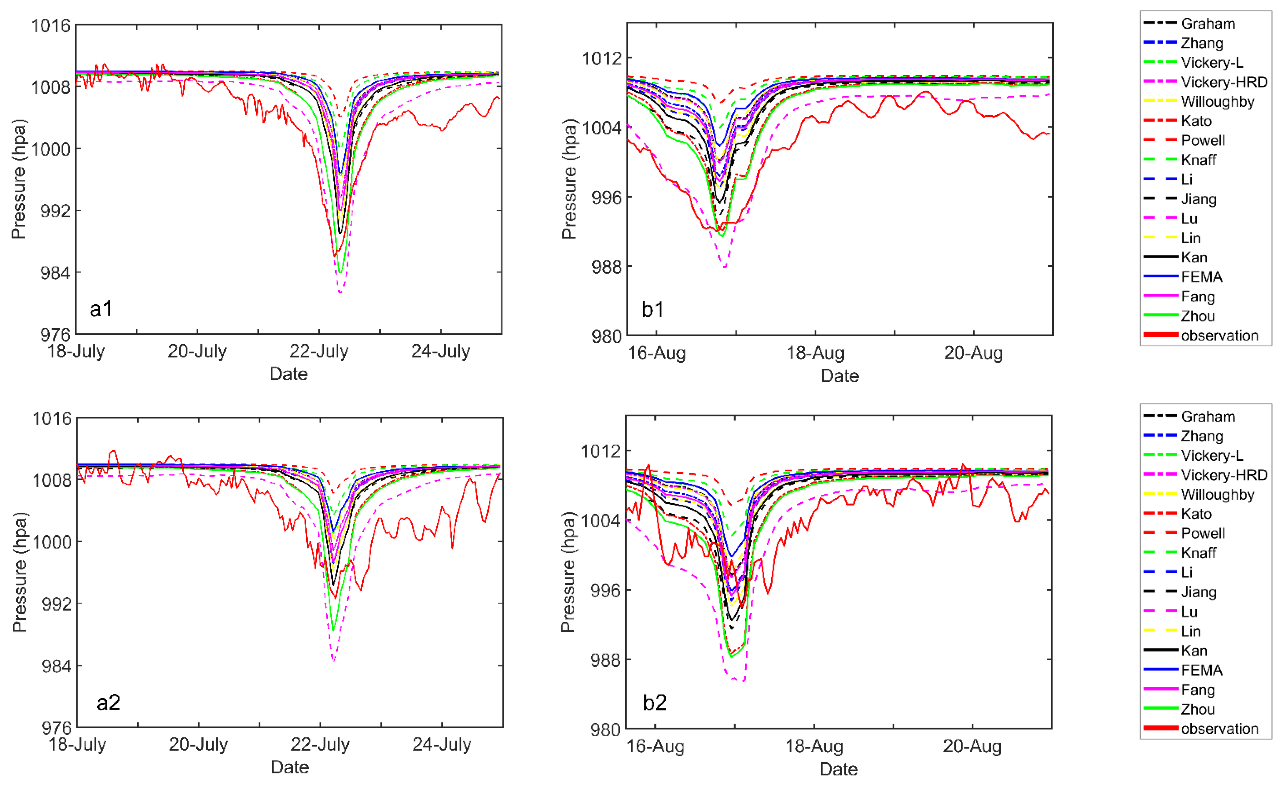
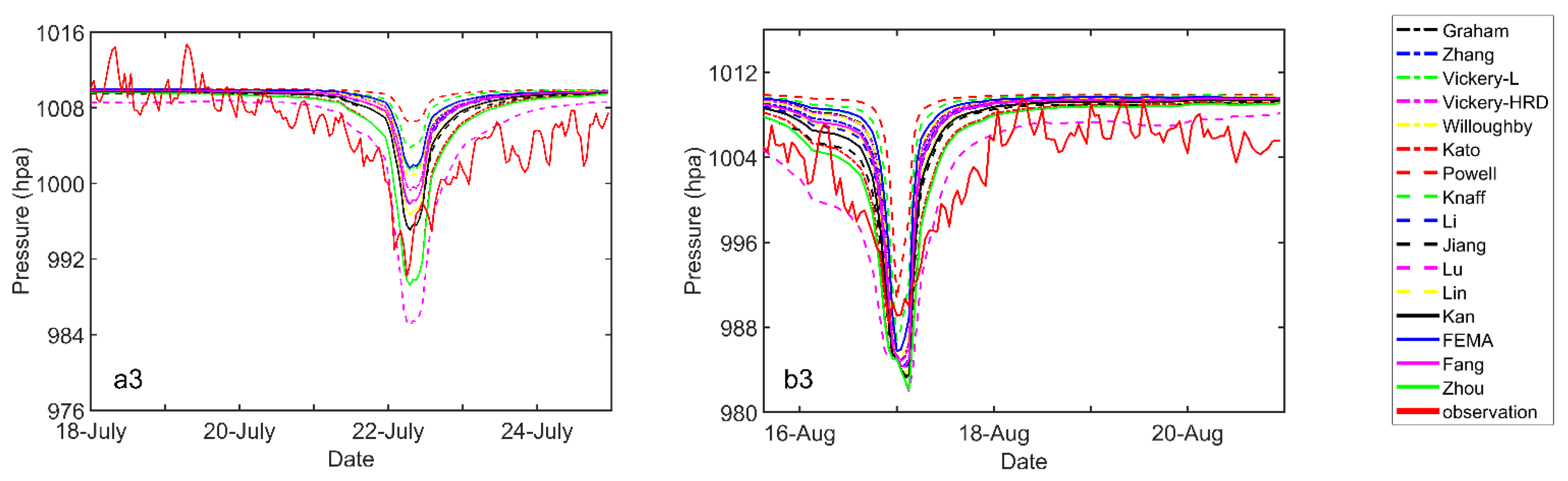
3.1. Comparison of Pressure at Observational Stations

Tropical cyclone features clear sky, warm temperature, and low atmospheric pressure in its central region or the eye. The larger the gradient between the central pressure and the ambient pressure, the stronger the wind speed. When the typhoon center transitions into a new location, the $R_m$ value of each empirical formulation is computed based on model input and then fed into Equation (1) to generate a pressure profile over the computational domain and pressure values at three stations.

Figure 2 shows time series comparisons of pressure between the model results and the measurements at each station for tropical storm Ampil and Rumbia, respectively. The red solid line indicates a continuous fluctuation of the measured pressure over a constant baseline of ambient pressure. The center of tropical storm Ampil passed through Zhoushan archipelago in the middle of 22 July and produced a pressure trough at each station around the same time. The lowest pressure values measured at station 1, 2, and 3 are 986 hPa, 993 hPa, and 990 hPa, respectively. On the way to reaching or leaving the pressure trough, all sixteen $R_m$ formulations show a sharp drop or rebound, in contrast to a moderate decrease and a mild recovery in the measurements. Both the 3- or 6-h interval of the center location and the strong interaction between the typhoon and on-land atmospheric system prior to landing are likely to contribute the evident difference. In terms of overall fit to the measurements computed as error metrics in

Table 1. Error metrics of pressure at Station 1 for tropical storm Ampil and Rumbia.

	RMSE	COR	Bias	SI	RMSE	COR	Bias	SI
	Ampil Pressure Error at Station 1				Rumbia Pressure Error at Station 1
Graham	5.35	0.87	4.27	0.0032	6.77	0.88	6.04	0.0031
Zhang	5.06	0.87	4.04	0.0030	6.32	0.90	5.71	0.0027
Vickery-L	5.74	0.86	4.50	0.0035	7.17	0.88	6.34	0.0033
Vickery-HRD	5.79	0.90	4.50	0.0036	6.70	0.89	5.98	0.0030
Willoughby	4.71	0.89	3.79	0.0028	5.78	0.90	5.21	0.0025
Kato	3.52	0.91	2.72	0.0022	4.35	0.93	3.98	0.0018
Powell	6.86	0.84	5.13	0.0045	8.28	0.86	7.15	0.0042
Knaff	6.27	0.85	4.81	0.0040	7.66	0.88	6.72	0.0037
Li	4.97	0.88	3.94	0.0030	5.92	0.91	5.38	0.0025
Jiang	4.34	0.88	3.41	0.0027	4.85	0.92	4.44	0.0019
Lu	2.47	0.93	1.09	0.0022	2.08	0.96	1.77	0.0017
Lin	5.59	0.86	4.38	0.0035	6.80	0.89	6.08	0.0030
Kan	4.47	0.89	3.59	0.0027	5.43	0.91	4.96	0.0022
FEMA	5.79	0.86	4.53	0.0036	7.18	0.87	6.34	0.0034
Fang	5.02	0.87	4.00	0.0030	6.14	0.90	5.55	0.0026
Zhou	3.41	0.91	2.61	0.0022	4.02	0.94	3.66	0.0017

,

Table 2. Error metrics of pressure at Station 2 for tropical storm Ampil and Rumbia.

	RMSE	COR	Bias	SI	RMSE	COR	Bias	SI
	Ampil Pressure Error at Station 2				Rumbia Pressure Error at Station 2
Graham	5.67	0.74	4.50	0.0034	3.97	0.84	2.41	0.0031
Zhang	5.46	0.72	4.28	0.0034	3.57	0.85	2.08	0.0029
Vickery-L	5.94	0.74	4.69	0.0036	4.40	0.83	2.74	0.0034
Vickery-HRD	5.64	0.74	4.47	0.0034	3.91	0.84	2.35	0.0031
Willoughby	5.17	0.76	4.08	0.0032	3.16	0.85	1.57	0.0027
Kato	4.35	0.76	3.06	0.0031	2.49	0.88	0.33	0.0025
Powell	6.69	0.72	5.20	0.0042	5.62	0.81	3.60	0.0043
Knaff	6.30	0.71	4.93	0.0039	4.92	0.83	3.14	0.0038
Li	5.37	0.74	4.19	0.0033	3.27	0.86	1.76	0.0027
Jiang	4.88	0.74	3.71	0.0032	2.61	0.87	0.82	0.0025
Lu	3.50	0.79	1.46	0.0032	3.68	0.90	−2.42	0.0028
Lin	5.82	0.72	4.57	0.0036	4.03	0.84	2.47	0.0032
Kan	5.01	0.74	3.87	0.0032	2.89	0.86	1.33	0.0025
FEMA	5.97	0.74	4.71	0.0036	4.40	0.83	2.74	0.0034
Fang	5.42	0.74	4.25	0.0033	3.43	0.85	1.93	0.0028
Zhou	4.25	0.76	2.96	0.0030	2.45	0.88	0.02	0.0024

and

Table 3. Error metrics of pressure at Station 3 for tropical storm Ampil and Rumbia.

	RMSE	COR	Bias	SI	RMSE	COR	Bias	SI
	Ampil Pressure Error at Station 3				Rumbia Pressure Error at Station 3
Graham	4.63	0.78	3.33	0.0032	5.05	0.83	4.14	0.0029
Zhang	4.42	0.77	3.11	0.0031	4.77	0.84	3.84	0.0028
Vickery-L	4.94	0.78	3.54	0.0034	5.36	0.80	4.46	0.0030
Vickery-HRD	4.61	0.78	3.30	0.0032	5.00	0.83	4.08	0.0029
Willoughby	4.11	0.80	2.88	0.0029	4.32	0.86	3.34	0.0027
Kato	3.40	0.80	1.85	0.0028	3.48	0.91	2.29	0.0026
Powell	5.80	0.77	4.09	0.0041	6.46	0.72	5.50	0.0034
Knaff	5.36	0.76	3.81	0.0038	5.80	0.77	4.91	0.0031
Li	4.33	0.78	3.02	0.0031	4.49	0.86	3.54	0.0028
Jiang	3.85	0.79	2.51	0.0029	3.78	0.88	2.68	0.0027
Lu	3.09	0.83	0.22	0.0031	2.82	0.92	−0.33	0.0028
Lin	4.82	0.77	3.42	0.0034	5.11	0.82	4.21	0.0029
Kan	3.96	0.79	2.68	0.0029	4.15	0.88	3.16	0.0027
FEMA	4.97	0.78	3.56	0.0035	5.37	0.80	4.46	0.0030
Fang	4.38	0.78	3.08	0.0031	4.63	0.85	3.69	0.0028
Zhou	3.31	0.81	1.73	0.0028	3.29	0.91	2.00	0.0026

, Lu’s $R_m$ formulation performs the best, with the lowest RMSE = 3.02, Bias = 0.9233, and SI = 0.003 and highest COR = 0.85 averaged across three stations, and Zhou’s (RMSE = 3.6567, Bias = 2.4333, SI = 0.003, COR = 0.8267) and Kato’s (RMSE = 3.7567, Bias = 2.5433, SI = 0.003, COR = 0.8233) formulations rank the second and third, respectively. However, in terms of the extreme value that the $R_m$ formulation can reach, Lu tends to overestimate the minimum pressure the most, although this drawback taking place for a short time range does not deteriorate the error metrics much.

The center of tropical cyclone Rumbia passed through Zhoushan archipelago around 17 August. Since the intensity of Rumbia was relatively weak, it produced a relatively broad pressure trough at station 1, with a minimum value of 992 hPa, a less distinct trough at station 2 with a minimum value of 993 hPa, and a normal pressure drop at station 3 with a minimum value of 989 hPa. There was a low-pressure system following typhoon Rumbia causing mild drops in measurements at all three stations after August 20. Among the 16 empirical formulations, Lu’s $R_m$ again yielded the overall best performance with averaged RMSE = 2.86, COR = 0.93, Bias = 1.5, and negligible difference in SI across all three stations. Zhou’s (RMSE = 3.25, COR = 0.91, Bias = 1.89) and Kato’s (RMSE = 3.44, COR = 0.91, Bias = 2.2) formulations rank second and third best, respectively, in reproducing atmospheric pressure in the event of Rumbia.

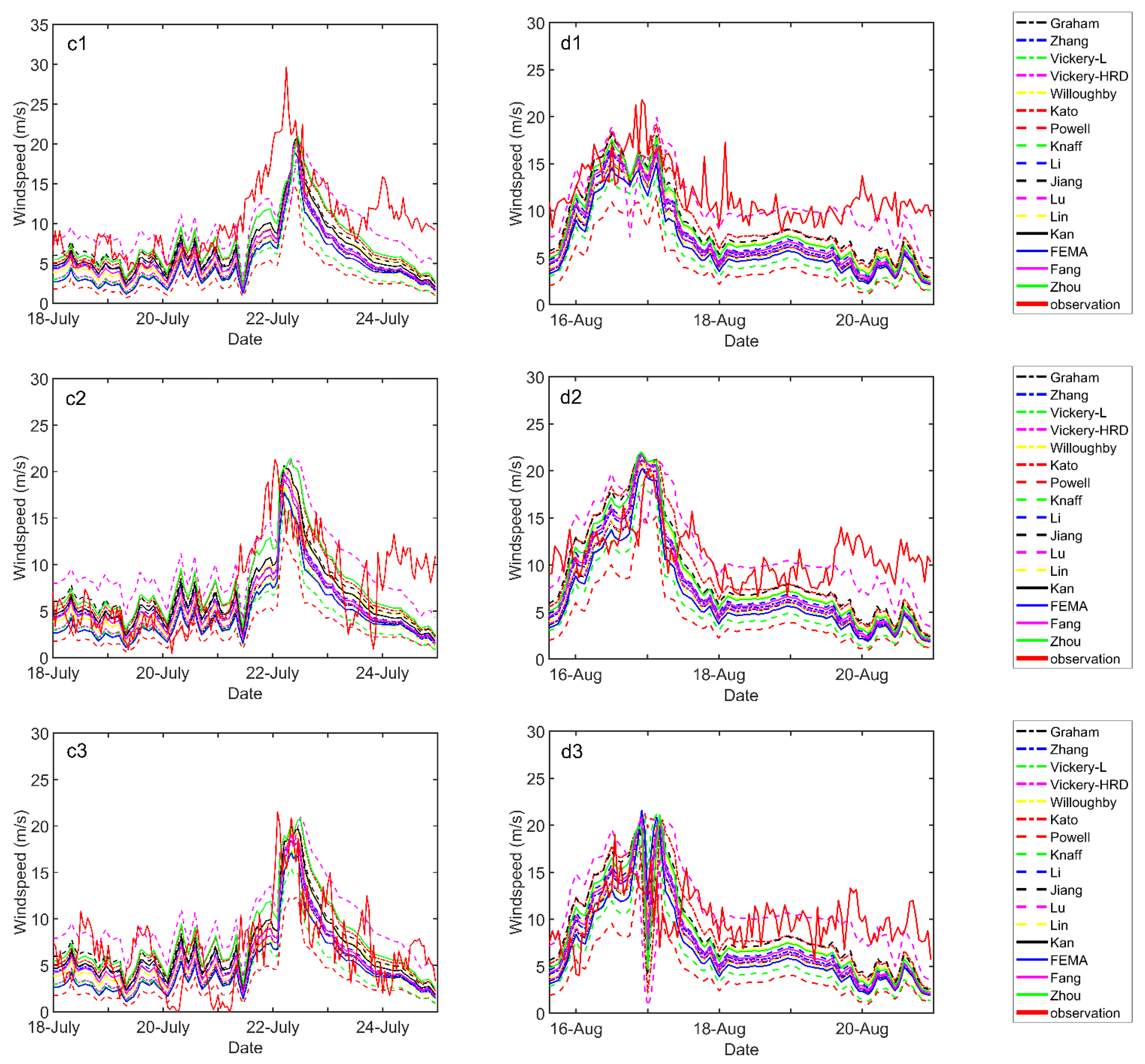
3.2. Comparison of Wind Speed at Observational Stations

Based on the magnitude of maximum sustained winds, in China, tropical cyclones are categorized into six scales: tropical depression (10.8~17.1 m/s), tropical storm (17.2~24.4 m/s), strong tropical storm (24.5~32.6 m/s), typhoon (32.7~41.4 m/s), strong typhoon (41.5~50.9 m/s), and super typhoon (51.0 m/s and above). Lower central pressure and steeper pressure gradient can usually yield higher wind speed. Tropical cyclones Ampil and Rumbia belong to the scale of the tropical storms, and the wind magnitude of Ampil is slightly higher than the one of Rumbia, owing to its lower minimum central pressure. In the Holland10 model, the radius of maximum wind speed $R_m$ not only influences the wind profile from the pressure field through Equation (1), but also modifies the wind profile through Equations (5) and (6) directly.

Figure 3 shows time series of wind speed computed from the H10 model with 16 $R_m$ formulations input, respectively, in comparison to measurements at station 1, 2, and 3. In the event of Ampil, the maximum values of wind speed measured at station 1, 2, and 3 were 29 m/s, 21 m/s, and 21 m/s, respectively. The peaks in the time series of the measurements arrived several hours early at all three stations compared to those in the model. This time lag can also be observed from the time series of pressure comparison in Figure 2(a1–a3). The systematic error is possibly associated with less accurate track location and a deformation of wind profile from circular to elliptical shape before landfall. After reaching the peak, the measured wind speed does not recover to the environmental level at the same rate of the computed results because of the involvement of other background atmospheric processes. The computed error indices listed in

Table 4. Error metrics of wind speed at Station 1 for tropical storm Ampil and Rumbia.

	RMSE	COR	Bias	SI	RMSE	COR	Bias	SI
	Ampil Wind Speed Error at Station 1				Rumbia Wind Speed Error at Station 1
Graham	6.01	0.79	−5.13	0.31	5.58	0.79	−5.08	0.19
Zhang	5.59	0.73	−4.36	0.34	5.31	0.78	−4.70	0.21
Vickery-L	6.30	0.78	−5.41	0.31	6.00	0.79	−5.56	0.19
Vickery-HRD	5.88	0.78	−4.92	0.31	5.49	0.79	−4.98	0.19
Willoughby	5.16	0.78	−4.04	0.31	4.53	0.78	−3.83	0.20
Kato	4.44	0.73	−2.72	0.34	3.94	0.77	−2.92	0.22
Powell	7.84	0.77	−7.01	0.34	7.85	0.78	−7.58	0.17
Knaff	6.92	0.73	−5.93	0.35	6.82	0.78	−6.45	0.19
Li	5.39	0.72	−4.05	0.35	4.93	0.78	−4.23	0.21
Jiang	4.78	0.70	−3.07	0.36	4.10	0.77	−3.19	0.21
Lu	3.99	0.64	−0.68	0.38	2.99	0.65	−1.06	0.23
Lin	6.05	0.72	−4.90	0.35	5.74	0.78	−5.22	0.20
Kan	5.03	0.73	−3.61	0.34	4.58	0.78	−3.79	0.21
FEMA	6.34	0.79	−5.46	0.31	5.99	0.79	−5.56	0.19
Fang	5.50	0.73	−4.26	0.34	5.09	0.78	−4.45	0.21
Zhou	4.32	0.72	−2.46	0.35	3.73	0.76	−2.63	0.22

,

Table 5. Error metrics of wind speed at Station 2 for tropical storm Ampil and Rumbia.

	RMSE	COR	Bias	SI	RMSE	COR	Bias	SI
	Ampil Wind Speed Error at Station 2				Rumbia Wind Speed Error at Station 2
Graham	4.30	0.68	−2.63	0.44	5.29	0.63	−3.72	0.34
Zhang	4.15	0.61	−1.81	0.49	5.18	0.62	−3.28	0.36
Vickery-L	4.49	0.68	−2.94	0.44	5.54	0.63	−4.26	0.32
Vickery-HRD	4.21	0.67	−2.42	0.45	5.23	0.63	−3.62	0.34
Willoughby	3.78	0.68	−1.50	0.45	4.62	0.61	−2.39	0.36
Kato	3.78	0.64	−0.04	0.49	4.49	0.58	−1.42	0.39
Powell	5.76	0.66	−4.57	0.46	7.01	0.63	−6.55	0.25
Knaff	5.03	0.61	−3.46	0.48	6.19	0.62	−5.20	0.30
Li	4.04	0.60	−1.51	0.49	4.93	0.61	−2.78	0.37
Jiang	3.89	0.59	−0.50	0.50	4.46	0.60	−1.67	0.37
Lu	4.43	0.59	2.12	0.51	3.80	0.48	0.47	0.34
Lin	4.40	0.60	−2.40	0.48	5.42	0.62	−3.85	0.35
Kan	3.90	0.62	−1.03	0.49	4.78	0.60	−2.31	0.38
FEMA	4.51	0.68	−2.99	0.44	5.53	0.63	−4.26	0.32
Fang	4.07	0.62	−1.73	0.48	5.03	0.61	−3.02	0.36
Zhou	3.81	0.63	0.22	0.50	4.36	0.57	−1.11	0.38

and

Table 6. Error metrics of wind speed at Station 3 for tropical storm Ampil and Rumbia.

	RMSE	COR	Bias	SI	RMSE	COR	Bias	SI
	Ampil Wind Speed Error at Station 3				Rumbia Wind Speed Error at Station 3
Graham	3.62	0.70	−1.75	0.46	4.90	0.50	−2.95	0.38
Zhang	3.35	0.68	−0.96	0.47	4.80	0.49	−2.62	0.39
Vickery-L	3.73	0.70	−2.06	0.45	5.16	0.51	−3.37	0.38
Vickery-HRD	3.51	0.70	−1.55	0.46	4.84	0.50	−2.86	0.38
Willoughby	3.24	0.70	−0.64	0.46	4.27	0.48	−1.80	0.38
Kato	3.49	0.68	0.77	0.50	4.33	0.42	−1.11	0.41
Powell	4.86	0.68	−3.70	0.46	6.53	0.48	−5.29	0.37
Knaff	4.09	0.67	−2.60	0.46	5.80	0.49	−4.19	0.39
Li	3.22	0.69	−0.66	0.46	4.57	0.48	−2.16	0.39
Jiang	3.14	0.71	0.35	0.46	4.22	0.45	−1.20	0.39
Lu	4.30	0.69	2.87	0.47	4.24	0.30	0.73	0.41
Lin	3.50	0.68	−1.54	0.46	5.05	0.50	−3.06	0.39
Kan	3.24	0.69	−0.19	0.47	4.45	0.47	−1.80	0.40
FEMA	3.75	0.70	−2.11	0.45	5.15	0.50	−3.36	0.38
Fang	3.28	0.69	−0.87	0.46	4.66	0.49	−2.37	0.39
Zhou	3.50	0.69	1.03	0.49	4.26	0.41	−0.82	0.41

indicate the performance of all 16 $R_m$ formulations. At station 1, Zhou (RMSE = 4.32, Bias = −2.46, SI = 0.35), Kato (RMSE = 4.44, Bias = −2.72, SI = 0.34), and Lu (RMSE = 3.99, Bias = −0.68, SI = 0.38) perform better in a similar way, in spite of their slightly lower correlation coefficient. At station 2, Willoughby (RMSE = 3.78, Bias = −1.5, SI = 0.45), Kato (RMSE = 3.78, Bias = −0.04, SI = 0.49), and Zhou (RMSE = 3.81, Bias = 0.22, SI = 0.5) rank as the top three formulations with better agreement on the measurements. At station 3, all 16 $R_m$ formulations show similar performance, with RMSE ranging between 3 to 5, COR around 0.7, SI between 0.45 to 0.5, and Bias varying between −4 to 2. In the average of metrics across three stations, Zhou (RMES = 3.88, Bias = −0.4), Kato (RMES = 3.9, Bias = −0.66), and Jiang (RMES = 3.94, Bias = −1.07) excel in RMSE and Bias indices with mediocre scores in the other two indices.

In the event of Rumbia, the measured wind speed slowly reduced to about 10 m/s after the peak arrival at around 0′o clock on August 17 and then was sustained due to the involvement of another atmospheric process; this trend is consistent with the measured pressure shown in Figure 2(b1–b3). Considering the process of the tropical cyclone alone, the modelled wind speed falls quicker than the measurements. A systematic sudden drop in the modelled wind speed is probably related to a 120° swerve of the center location close to station 3 (Figure 1d). At station 1, Lu (RMSE = 2.99, Bias = −1.06), Zhou (RMSE = 3.73, Bias = −2.63), and Kato (RMSE = 3.94, Bias = −2.92) better agree with the measurements in terms of RMSE and Bias, although Lu’s COR = 0.65 ranks last among all 16 formulations. The same performance is also achieved at station 2 for Lu (RMSE = 3.8, Bias = 0.47, COR = 0.48), Zhou (RMSE = 4.36, Bias = −1.11, COR = 0.57), and Kato (RMSE = 4.49, Bias = −1.42, COR = 0.58). At station 3, correlations from all 16 formulations are less than 0.5, leading to irregular ranks in indices. On average, in terms of performance across three stations, Lu (RMSE = 3.68, Bias = 0.05), Zhou (RMSE = 4.12, Bias = −1.52), and Kato (RMSE = 4.25, Bias = −1.82) rank as the top three, respectively.

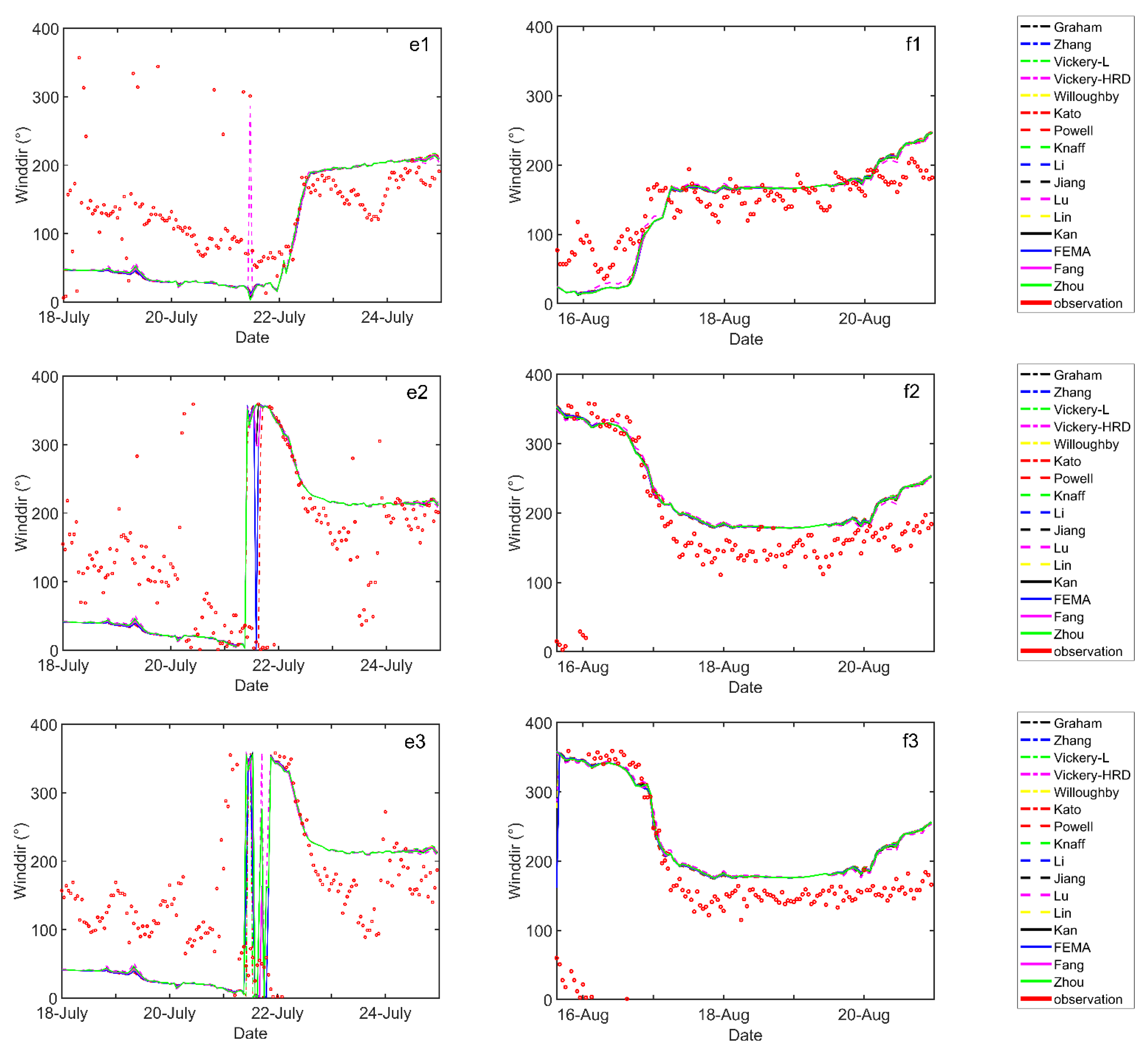
3.3. Comparison of Wind Direction at Observational Stations

Wind direction, defined as the arctangent of the east/west component vs. the north/south component, is a sensitive parameter with many complicated influencing factors. The tracks of tropical storms Ampil and Rumbia passed right between station 1 and station 2 (or 3) and produced distinct characteristics of wind direction variation on measurements from each group of stations (Figure 1). In the event of Ampil, station 1 experienced south wind which transitioned into east wind counterclockwise around 22 July and then quickly swung back to SSW clockwise with undulations around 24 July. Stations 2 and 3 also experienced southern wind in the beginning, but it turned to north wind counterclockwise on about 22 July and then continued the rotation to SSW with direction variation on 24 July. Under the same environment setup, all 16 $R_m$ formulations contribute to the east/west and north/south components equally and generate basically the same variation in wind direction. The evident direction differences between the modeled and the measured prior to the tropical storm arrival are due to the dominant background wind field, which is not considered in the H10 model. In the event of Rumbia, station 1 experienced eastern wind which transitioned into south or SSW wind clockwise. Meanwhile, station 2 and 3 experienced northern wind on August 16 and then the wind direction turned to south counterclockwise. All 16 $R_m$ formulations yield the same numerical results, which basically follow the general trend of the measured wind direction with visible error in different time spans. Since all $R_m$ formulations perform the same in the time series comparison in Figure 4, we do not consider wind direction in the following error analysis.

3.4. Error Analysis

The 16 $R_m$ formulations generate a spectrum of time series of pressure and wind speed at three stations through the running of the H10 model for tropical cyclone events Ampil and Rumbia to be compared with the observational records. Their performance is evaluated by four indices: RMSE, COR, Bias, and SI (Table 1, Table 2, Table 3, Table 4, Table 5 and Table 6). The COR measures the similarity in trend in the time series form, and low correlation does not necessarily mean high deviation in individual magnitude. Moreover, the time series generated by the 16 $R_m$ formulations shown in Figure 2 and Figure 3 mainly differ in magnitude, not in trend, and the COR cannot efficiently reflect their performance. Therefore, we do not consider the index COR in the following error analysis. Among the three indices remaining, the value of SI is too small and is not at the same magnitude as RMSE and Bias. To produce the three indices at the same amount of weight in evaluating, we multiply 1000 for SI in pressure comparison and 10 in wind speed comparison. Therefore, for each event (Ampil or Rumbia), and each physical variable (pressure or wind speed), the error listed in

Table 7. Comprehensive error (CE) of pressure and wind speed for typhoon Ampil and Rumbia.

Rm Formulation	Typhoon Ampil			Typhoon Rumbia
	Error in Wind Speed	Error in Pressure	Comprehensive Error	Error in Wind Speed	Error in Pressure	Comprehensive Error
Graham	3.96	4.2	4.08	4.07	4.16	4.12
Zhang	3.69	4.0	3.85	3.94	3.85	3.90
Vickery-L	4.12	4.4	4.26	4.31	4.46	4.39
Vickery-HRD	3.86	4.3	4.08	4.02	4.11	4.07
Willoughby	3.41	3.7	3.56	3.42	3.47	3.45
Kato	3.18	3.0	3.09	3.15	2.65	2.90
Powell	5.15	5.2	5.18	5.41	5.39	5.40
Knaff	4.55	4.8	4.68	4.83	4.86	4.85
Li	3.54	3.9	3.72	3.70	3.60	3.65
Jiang	3.21	3.5	3.36	3.18	2.92	3.05
Lu	3.55	2.3	2.93	2.57	2.27	2.42
Lin	3.96	4.3	4.13	4.19	4.20	4.20
Kan	3.34	3.6	3.47	3.51	3.26	3.39
FEMA	4.14	4.5	4.32	4.30	4.48	4.39
Fang	3.62	4.0	3.81	3.80	3.73	3.77
Zhou	3.18	2.9	3.04	3.00	2.46	2.73

for all three stations is calculated from Table 1, Table 2, Table 3, Table 4, Table 5 and Table 6 as

$$Error=\frac{1}{3}\left(\overline{Bias}+\overline{RMSE}+x\overline{SI}\right)$$

(35)

where $x=1000$ when $SI$ is measuring pressure and $x=10$ when $SI$ is measuring wind speed. If we consider both events and physical variables as having the same amount of weight, the average of the two error values provide a comprehensive error for each event listed in Table 7.

In the Ampil event, Lu’s formulation performs the best in reproducing the pressure time series, but falls short of reaching good agreement with the wind speed. The first place in pressure with dominant advantage and seventh place in wind speed give it the top rank in the list of comprehensive error among the 16 $R_m$ formulations. Zhou’s formulation ranks first in wind speed comparison and second in pressure, leading to a second place in the comprehensive error list. Kato’s formulation provides the same best performance as Zhou’s formulation in wind speed comparison and ranks third in the pressure comparison, resulting in a third place among all 16 formulations. Jiang’s formulation follows immediately after Kato’s and ranks fourth place in the comprehensive error list. In the Rumbia event, Lu, Zhou, Kato, and Jiang’s formulation rank the first, second, third, and fourth place, respectively, in both the wind speed and pressure comparison, leading to the same positions as in the comprehensive error list. The Ampil and Rumbia events were independent tropical storm events in 2018 and had completely different characteristics in terms of distribution of pressure and the wind speed recorded at three stations. Nevertheless, both events give rise to the same rank in the comprehensive error, which strongly supports the reasonability of the proposed methodology and credibility of the optimal formulation list.

3.5. Discussion

The investigation of the evidence in support of the lowest comprehensive error being produced by Lu’s $R_m$ formulation reveals that the plausible first rank is simply an occasional incident. Since the tropical cyclones Ampil and Rumbia are relatively weak in intensity, the measured pressure and wind speed are heavily saturated by background atmospheric processes, especially on the sections 24 h before and after the peak/trough region, and the characteristics of the tropical storms were distorted to a certain extent. Meanwhile, it so happened that Lu’s $R_m$ formulation usually yields the best performance on saturated sections. This coincidence results in the best agreement on pressure primarily and leads to the top rank in terms of comprehensive error for Lu’s formulation. It can also be implied that the radius of the maximum wind speed from Lu’s prediction for Ampil and Rumbia must be significantly larger than the realistic one. From a conservative perspective, Lu’s $R_m$ formulation is still recommended to outline the worst case in hazard mitigation. Meanwhile, from the perspective of accuracy in modeling physical variables, Zhou, Kato, and Jiang, with realistic predictions on $R_m$ and steadily good performance, are recommended to be optimal formulations for the Holland10 modeling of tropical cyclones over Zhoushan archipelago in the East China Sea.

4. Conclusions

In comparison to numerical weather prediction models, parametric wind models are more efficient in reconstructing pressure and wind fields of tropical cyclone events and have been extensively adopted in storm surge-related coastal hazards and emergency management. As one of the representative realizations, the Holland10 model, inheriting essentials of its predecessor H80 model, has been implemented more frequently. As the only undetermined input parameter sensitive to interest regions, the radius of maximum wind speed can effectively influence the model performance, but optimal empirical formulations in generating $R_m$ are not yet known over the Zhoushan archipelago, in the East China Sea. In this paper, 16 $R_m$ formulations are compiled into the H10 model to produce a time series of pressure, wind speed, and wind direction at three observational stations in the historical tropical cyclones events of Ampil and Rumbia, both of which took place in 2018. Based on the recorded data at three stations, the performance of numerical results is evaluated through error metrices, including RMSE, Bias, COR and SI, and optimal $R_m$ formulations are selected and recommended in terms of the opposite perspective.

The time series comparison in pressure and wind speed among all 16 proposed $R_m$ empirical formulations indicates that the radius of maximum wind speed mainly alters the magnitude, instead of the variation pattern. Additionally, the $R_m$ computed from different formulations yields the same wind direction, owing to the same contribution on each velocity component. Based on the comprehensive error synthesized from RMSE, Bias, and SI, Lu’s, Zhao’s, and Kato’s formulations yield the top three minimum error rankings in comparison to onsite measurements and Jiang’s formulation ranks the fourth. However, the relatively weak nature of the tropical cyclone events Ampil and Rumbia induces saturation into the background environment in measurements, and the $R_m$ performance evaluated under this baseline should be perceived cautiously. In Lu’s formulation, the radius of maximum wind speed is expressed in terms of pressure drop in an exponential form, and the corresponding time series at each station usually constitutes the lower bound in pressure and upper bound in wind speed. The corresponding feature indicates that Lu’s formulation provides the most extreme prediction on the radius of maximum wind speed. It is recommended that Lu’s formulation can be applied to produce the most conservative results, and Zhao’s, Kato’s, and Jiang’s formulations are suitable to depict the tropical cyclone more accurately.

References

1. Bell, S.S.; Chand, S.S.; Camargo, S.J.; Tory, K.J.; Turville, C.; Ye, H. Western North Pacific tropical cyclone tracks in CMIP5 models: Statistical assessment using a model-independent detection and tracking scheme. J. Clim. 2019, 32, 7191–7208. [Google Scholar] [CrossRef] [Green Version]
2. Wang, C.; Wu, L.G. Influence of future tropical cyclone track changes on their basin-wide intensity over the Western North Pacific: Downscaled CMIP5 Projections. Adv. Atmos. Sci. 2015, 32, 613–623. [Google Scholar] [CrossRef]
3. Benjamin, S.G.; Weygandt, S.S.; Brown, J.M.; Hu, M.; Manikin, G.S.; Alexander, C.R.; Smirnova, T.G.; Olson, J.B.; Bennett Vanessa, C.C.; Mulligan Ryan, P. Evaluation of surface wind fields for prediction of directional ocean wave spectra during hurricane Sandy. Coast. Eng. 2017, 125, 1–15. [Google Scholar] [CrossRef] [Green Version]
4. Davis, C.; Wang, W.; Chen, S.Y.; Chen, Y.; Corbosiero, K.; DeMaria, M.; Dudhia, J.; Holland, G.; Klemp, J.; Michalakes, J.; et al. Prediction of Landfalling Hurricanes with the Advanced Hurricane WRF Model. Mon. Weather Rev. 2008, 136, 1990–2005. [Google Scholar] [CrossRef] [Green Version]
5. Frank, W.M.; Ritchie, E.A. Effects of Vertical Wind Shear on the Intensity and Structure of Numerically Simulated Hurricanes. Mon. Weather Rev. 2001, 129, 2249–2269. [Google Scholar] [CrossRef]
6. Islam, T.; Srivastava, P.K.; Rico-Ramirez, M.A.; Dai, Q.; Gupta, M.; Singh, S.K. Tracking a tropical cyclone through WRF–ARW simulation and sensitivity of model physics. Nat. Hazards 2015, 76, 1473–1495. [Google Scholar] [CrossRef]
7. Shaw, W.J.; Berg, L.K.; Cline, J.; Draxl, C.; Djalalova, I.; Grimit, E.P.; Lundquist, J.K.; Marquis, M.; McCaa, J.; Olson, J.B.; et al. The Second Wind Forecast Improvement Project (WFIP2): General Overview. Bull. Am. Meteorol. Soc. 2019, 100, 1687–1699. [Google Scholar] [CrossRef]
8. Wong, M.L.M.; Chan, J.C.L. Tropical Cyclone Intensity in Vertical Wind Shear. J. Atmos. Sci. 2010, 61, 1859–1876. [Google Scholar] [CrossRef]
9. Davis, C.; Wang, W.; Dudhia, J.; Torn, R. Does Increased Horizontal Resolution Improve Hurricane Wind Forecasts? Weather Forecast. 2010, 25, 1826–1841. [Google Scholar] [CrossRef]
10. Pandey, S.; Rao, A.D. An improved cyclonic wind distribution for computation of storm surges. Nat. Hazards 2018, 92, 93–112. [Google Scholar] [CrossRef]
11. Rao, D.V.B.; Srinivas, D. Multi-Physics ensemble prediction of tropical cyclone movement over Bay of Bengal. Nat. Hazards 2014, 70, 883–902. [Google Scholar] [CrossRef]
12. Prasad Rao Anisetty, S.K.A.V.; Huang, C.Y.; Chen, S.Y. Impact of FORMOSAT-3/COSMIC radio occultation data on the prediction of super cyclone Gonu (2007): A case study. Nat. Hazards 2014, 70, 1209–1230. [Google Scholar] [CrossRef]
13. Deppermann, C.E. Notes on the Origin and Structure of Philippine Typhoons. Bull. Am. Meteorol. Soc. 1947, 28, 399–404. [Google Scholar] [CrossRef] [Green Version]
14. Jelesnianski, C.P. Numerical computations of storm surges without bottom stress. Mon. Weather Rev. 1966, 94, 374–394. [Google Scholar] [CrossRef]
15. Emanuel, K.; Rotunno, R. Self-Stratification of Tropical Cyclone Outflow. Part I: Implications for Storm Structure. J. Atmos. Sci. 2011, 68, 2236–2249. [Google Scholar] [CrossRef]
16. Emanuel, K. Tropical cyclone energetics and structure. In Atmospheric Turbulence and Mesoscale Meteorology; Fedorovich, E., Rotunno, R., Stevens, B., Eds.; Cambridge University Press: Cambridge, UK, 2004; pp. 165–192. [Google Scholar]
17. Holland, G.J.; Belanger, J.I.; Fritz, A. A Revised Model for Radial Profiles of Hurricane Winds. Mon. Weather Rev. 2010, 138, 4393–4401. [Google Scholar] [CrossRef]
18. Holland, G.J. An Analytic Model of the Wind and Pressure Profiles in Hurricanes. Mon. Weather Rev. 1980, 108, 1212–1218. [Google Scholar] [CrossRef]
19. Hu, K.; Chen, Q.; Kimball, S.K. Consistency in hurricane surface wind forecasting: An improved parametric model. Nat. Hazards 2012, 61, 1029–1050. [Google Scholar] [CrossRef]
20. Knaff, J.A.; Zehr, R.M. Reexamination of tropical cyclone wind—Pressure relationships. Weather Forecast 2007, 22, 71–88. [Google Scholar] [CrossRef]
21. Wijnands, J.S.; Qian, G.; Kuleshov, Y. Spline-based modelling of near-surface wind speeds in tropical cyclones. Appl. Math. Model. 2016, 40, 8685–8707. [Google Scholar] [CrossRef]
22. Willoughby, H.E.; Darling, R.W.R.; Rahn, M.E. Parametric representation of the primary hurricane vortex. Part II: A new family of sectionally continuous profiles. Mon. Weather Rev. 2006, 134, 1102–1120. [Google Scholar] [CrossRef] [Green Version]
23. Lin, N.; Chavas, D. On hurricane parametric wind and applications in storm surge modeling. J. Geophys. Res. Atmos. 2012, 117. [Google Scholar] [CrossRef]
24. Meza-Padilla, R.; Appendini, C.M.; Pedrozo-Acuña, A. Hurricane-induced waves and storm surge modeling for the Mexican coast. Ocean Dyn. 2015, 65, 1199–1211. [Google Scholar] [CrossRef]
25. Shao, Z.X.; Liang, B.C.; Li, H.J.; Wu, J.X.; Wu, Z.H. Blended wind fields for wave modeling of tropical cyclones in the South China Sea and East China Sea. Appl. Ocean. Res. 2018, 71, 20–33. [Google Scholar] [CrossRef]
26. Lin, N.; Emanuel, K.A.; Smith, J.A.; Vanmarcke, E. Risk assessment of hurricane storm surge for New York City. J. Geophys. Res. Atmos. 2010, 115. [Google Scholar] [CrossRef] [Green Version]
27. Lin, N.; Lane, P.; Emanuel, K.A.; Sullivan, R.M.; Donnelly, J.P. Heightened hurricane surge risk in northwest Florida revealed from climatological-hydrodynamic modeling and paleorecord reconstruction. J. Geophys. Res. Atmos. 2014, 119, 8606–8623. [Google Scholar] [CrossRef] [Green Version]
28. Rey, W.; Mendoza, T.E.; Salles, P.; Zhang, K.; Teng, Y.; Miguel, A.; Franklin, G.L. Hurricane flood risk assessment for the Yucatan and Campeche State coastal area. Nat. Hazards 2019, 96, 1041–1065. [Google Scholar] [CrossRef]
29. Li, N.; Roeber, V.; Yamazaki, Y.; Heitmann, T.; Bai, Y.F.; Cheung, K.F. Integration of coastal inundation modeling from storm tides to individual waves. Ocean Model. 2014, 83, 26–42. [Google Scholar] [CrossRef]
30. Li, N.; Yamazaki, Y.; Roeber, V.; Cheung, K.F.; Chock, G. Probabilistic mapping of storm-induced coastal inundation for climate change adaptation. Coast. Eng. 2018, 133, 126–1141. [Google Scholar] [CrossRef]
31. Phadke, A.C.; Martino, C.D.; Cheung, K.F.; Houston, S.H. Modeling of tropical cyclone winds and waves for emergency management. Ocean Eng. 2003, 30, 553–578. [Google Scholar] [CrossRef]
32. Dietrich, J.C.; Tanaka, S.; Westerink, J.J.; Dawson, C.N.; Luettich, R.A., Jr.; Zijlema, M.; Holthuijsen, L.H.; Smith, J.M.; Westerink, L.G.; Westerink, H.J. Performance of the Unstructured-Mesh, SWAN+ADCIRC Model in Computing Hurricane Waves and Surge. J. Sci. Comput. 2012, 52, 468–497. [Google Scholar] [CrossRef]
33. Muis, S.; Verlaan, M.; Winsemius, H.; Aerts, J.; Ward, P. A global reanalysis of storm surges and extreme sea levels. Nat. Commun. 2016, 7, 11969. [Google Scholar] [CrossRef] [Green Version]
34. Orton, P.M.; Conticello, F.R.; Cioffi, F.; Hall, T.M.; Georgas, N.; Lall, U.; Blumberg, A.F.; MacManus, K. Flood hazard assessment from storm tides, rain and sea level rise for a tidal river estuary. Nat. Hazards 2020, 102, 729–757. [Google Scholar] [CrossRef]
35. Das, Y. Parametric modeling of tropical cyclone wind fields in India. Nat. Hazards 2018, 93, 1049–1084. [Google Scholar] [CrossRef]
36. Zheng, P.; Li, M.; Wang, C.; Wolf, J.; Chen, X.; de Dominicis, M.; Yao, P.; Hu, Z. Tide-surge interaction in the Pearl River Estuary: A Case Study of Typhoon Hato. Front. Mar. Sci. 2020, 7, 236. [Google Scholar] [CrossRef]
37. Condon, A.J.; Sheng, Y.P. Evaluation of coastal inundation hazard for present and future climates. Nat. Hazards 2012, 62, 345–373. [Google Scholar] [CrossRef] [Green Version]
38. Guo, L.L.; Sheng, J.Y. Statistical estimation of extreme ocean waves over the eastern Canadian shelf from 30-year numerical wave simulation. Ocean Dyn. 2015, 65, 1489–1507. [Google Scholar] [CrossRef]
39. Ng, K.S.; Leckebusch, G.C. A new view on the risk of typhoon occurrence in the western North Pacific. Nat. Hazards Earth Syst. Sci. 2021, 21, 663–682. [Google Scholar] [CrossRef]
40. Holland, G. A Revised Hurricane Pressure-Wind Model. Mon. Weather Rev. 2008, 136, 3432–3445. [Google Scholar] [CrossRef] [Green Version]
41. Fang, Y.P.; Enrico, Z. An adaptive robust framework for the optimization of the resilience of interdependent infrastructures under natural hazards. Eur. J. Oper. Res. 2019, 276, 1119–1136. [Google Scholar] [CrossRef]
42. Dominicis, M.D.; Wolf, J.; Jevrejeva, S.; Zheng, P.; Hu, Z. Future interactions between sea level rise, tides, and storm surges in the world’s largest urban area. Geophys. Res. Lett. 2020, 47, e2020GL087002. [Google Scholar] [CrossRef] [Green Version]
43. Kalourazi, M.Y.; Siadatmousavi, S.M.; Yeganeh-Bakhtiary, A.; Jose, F. Simulating tropical storms in the Gulf of Mexico using analytical models. Oceanologia 2020, 62, 173–189. [Google Scholar] [CrossRef]
44. Murty, P.; Rao, A.D.; Siva, S.K.; Pattabhi, R.R.E. Effect of Wave Radiation Stress in Storm Surge-Induced Inundation: A Case Study for the East Coast of India. Pure Appl. Geophys. 2020, 177, 2993–3012. [Google Scholar] [CrossRef]
45. Vijayan, L.; Huang, W.; Yin, K.; Ozguven, E.; Burns, S.; Ghorbanzadeh, M. Evaluation of parametric wind models for more accurate modeling of storm surge: A case study of Hurricane Michael. Nat. Hazards 2021, 106, 2003–2024. [Google Scholar] [CrossRef]
46. Fang, G.; Zhao, L.; Cao, S.; Ge, Y.; Pang, W. A novel analytical model for wind field simulation under typhoon boundary layer considering multi-field correlation and height-dependency. J. Wind. Eng. Ind. Aerodyn. 2018, 175, 77–89. [Google Scholar] [CrossRef]
47. Schloemer, R.W. Analysis and synthesis of hurricane wind patterns over Lake Okeechobee, Florida. In Hydrometeorological Rep. 31; Department of Commerce and U.S. Army Corps of Engineers, U.S. Weather Bureau: Washington, DC, USA, 1954; p. 49. [Google Scholar]
48. Powell, M.; Soukup, G.; Cocke, S.; Gulati, S.; Morisseau-Leroy, N.; Hamid, S.; Dorst, N.; Axe, L. State of Florida hurricane loss projection model: Atmospheric science component. J. Wind. Eng. Ind. Aerodyn. 2005, 93, 651–674. [Google Scholar] [CrossRef] [Green Version]
49. Vickery, P.J.; Masters, F.J.; Powell, M.D.; Wadhera, D. Hurricane hazard modeling: The past, present, and future. J. Wind. Eng. Ind. Aerodyn. 2009, 97, 392–405. [Google Scholar] [CrossRef]
50. Vickery, P.J.; Skerlj, P.F.; Twisdale, L.A. Simulation of Hurricane Risk in the U.S. Using Empirical Track Model. J. Struct. Eng. 2000, 126, 1222–1237. [Google Scholar] [CrossRef]
51. Levinson, D.H.; Knapp, K.R.; Kruk, M.C.J.H.; Kossin, J.P. The International Best Track Archive for Climate Stewardship (IBTrACS) Project: Overview of Methods and Indian Ocean Statistics. In Indian Ocean Tropical Cyclones and Climate Change; Charabi, Y., Ed.; Springer: Dordrecht, The Netherlands, 2010. [Google Scholar]
52. Harper, B.A.; Holland, G.J. An updated parametric model of tropical cyclone. In Proceedings of the 23rd Conference on Hurricanes and Tropical Meteorology, American Meteorological, Society, Dallas, TX, USA, 10–15 January 1999. [Google Scholar]
53. Graham, H.E.; Nunn, D.E. Meteorological considerations pertinent to standard project hurricane, Atlantic and Gulf coasts of the United States. In National Hurricane Research Project Report; Government Printing Office: Washington, DC, USA, 1959; Volume 33, pp. 20–39. [Google Scholar]
54. Zhang, L. Numerical Simulation of Winds and Waves in the South China Sea Based on different Typhoon Field Models. Master’s Thesis, Dalian Ocean University, Dalian, China, 2015; 78p. (In Chinese with English abstract). [Google Scholar]
55. Vickery, P.J.; Skerlj, P.F.; Steckley, A.C.; Twisdale, L.A. Hurricane Wind Field Model for Use in Hurricane Simulations. J. Struct. Eng. 2000, 126, 1203–1221. [Google Scholar] [CrossRef]
56. Willoughby, H.E.; Rahn, M.E. Parametric Representation of the Primary Hurricane Vortex. Part I: Observations and Evaluation of the Holland (1980) Model. Mon. Weather Rev. 2004, 132, 3033–3048. [Google Scholar] [CrossRef]
57. Powell, M.D.; Black, P.G. The relationship of hurricane reconnaissance flight-level wind measurements to winds measured by NOAA’s oceanic platforms. J. Wind. Eng. Ind. Aerodyn. 1990, 36, 381–392. [Google Scholar] [CrossRef]
58. Kato, F. Study on Risk Assessment of Storm Surge Flood, Technical Note of National Institute for Land and Infrastructure Management of Japan; No.275; National Institute for Land and Infrastructure Management: Tokyo, Japan, 2005.
59. Knaff, J.A.; Sampson, C.R.; DeMaria, M.; Marchok, T.P.; Gross, J.M.; McAdie, C.J. Statistical Tropical Cyclone Wind Radii Prediction Using Climatology and Persistence. Weather Forecast. 2007, 22, 781–791. [Google Scholar] [CrossRef]
60. Li, R.L. Prediction of Typhoon Extreme Wind Speeds Based on Improved Typhoon Key Parameters. Master’s Thesis, Harbin Institute of Technology, Harbin, China, 2007; 77p. (In Chinese with English Abstract). [Google Scholar]
61. Atkinson, G.D.; Holliday, C.R. Tropical cyclone minimum sea level pressure/maximum sustained wind relationship for the Western North Pacific. Mon. Weather Rev. 1977, 105, 421–427. [Google Scholar] [CrossRef] [Green Version]
62. Jiang, Z.H.; Hua, F.; Qu, P. A new tropical cyclone parameter adjustment scheme. Adv. Mar. Sci. 2008, 1, 1–7. (In Chinese) [Google Scholar]
63. Zhao, L.; Lu, A.; Zhu, L.; Cao, S.; Ge, Y. Near Ground Air Pressure of Landing Typhoon Measured Reconstruction and Its Impact on the Extreme Value Wind Velocity Evaluations of Engineering Fields. Available online: https://d.wanfangdata.com.cn/conference/9032185 (accessed on 26 May 2017).
64. Lin, W.; Fang, W.H. Study on the Regional Characteristics of Holland B coefficient in the Typhoon wind field model in the Northwest Pacific Ocean. Trop. Geogr. 2013, 33, 124–132, (In Chinese with English Abstract). [Google Scholar]
65. Kan, P.P. Simulation of Typhoon Pressure Field and Wind Field in Putuo District, Zhoushan City Based on Various Models. Master’s Thesis, East China Normal University, Shanghai, China, 2014; 84p. (In Chinese with English Abstract). [Google Scholar]
66. FEMA. Multi-Hazard Loss Estimation Methodology; Federal Emergency Management Agency: Washington, DC, USA, 2015.
67. Fang, W.; Chen, G.P.; Zhao, H.J.; Yan, S.C. A Comparative Study on the Calculation effect of maximum wind speed Radius on station wind wave. J. Waterw. Harb. 2017, 38, 574–580. (In Chinese) [Google Scholar]
68. Zhou, T.; Tan, Y.; Chu, A.; Zhang, C. Integrated model for astronomic tide and storm surge induced by typhoon for Ningbo coast. In Proceedings of the 28th International Ocean and Polar Engineering Conference, Sapporo, Japan, 10–15 June 2018; pp. 1124–1129. [Google Scholar]
Figure 1. Typhoon track information and corresponding intensity: (a) location of typhoon center and maximum wind speed for Ampil in computational domain; (b) location of typhoon center and maximum wind speed for Rumbia in computational domain; (c) Track information of typhoon Ampil in close-up view over Zhoushan archipelago; (d) Track information of typhoon Rumbia in close-up view over Zhoushan archipelago. Red, purple, and green triangle denotes observational station 1, 2, and 3, respectively.
Sustainability 13 11673 g001
Figure 2. Time series of pressure comparison between Holland10 computational results based on 16 R m formulations and onsite measurements at three stations for tropical storm Ampil and Rumbia: (a1a3) pressure comparison at station 1–3 for tropical storm Ampil; (b1b3) pressure comparison at station 1–3 for tropical storm Rumbia.
Sustainability 13 11673 g002aSustainability 13 11673 g002b
Figure 3. Time series of wind speed comparison between Holland10 computational results based on 16 R m formulations and onsite measurements at three stations for typhoon Ampil and Rumbia: (c1c3) wind speed comparison at stations 1–3 for tropical storm Ampil; (d1d3) windspeed comparison at stations 1–3 for tropical storm Rumbia.
Sustainability 13 11673 g003
Figure 4. Time series of wind direction comparison between H10 computational results based on 16 R m formulations and onsite measurements at three stations for typhoon Ampil and Rumbia: (e1e3) pressure comparison at stations 1–3 for tropical storm Ampil; (f1f3) pressure comparison at stations 1–3 for tropical storm Rumbia.
Sustainability 13 11673 g004