Abstract
Stormwater ponds are a common way to handle stormwater and are used to retain pollutants through sedimentation. The ponds resemble small natural lakes and will be colonized by flora and fauna. How design with respect to age, ratio between wet volume and reduced catchment area and land use influences the retention and how biodiversity is affected was examined. Age and ratio were determined in 135 and 59 ponds, respectively, and 12 of these ponds were selected for studies of dry weight (DW), organic matter (OM), total phosphorus (TP) and aluminum (Al), zinc (Zn), copper (Cu), chromium (Cr), cadmium (Cd) and lead (Pb) in the sediment. Invertebrate biodiversity was determined by Shannon–Wiener index (H’) and Pielou Evenness (J). DW, OM, TP and metals in the sediment close to the outlet of the ponds were influenced by pond age and the volume/area ratio whereas the sediment in the inlet area was more affected by the catchment type. Biodiversity increased with increasing ratio, while age had no effect on the sediment biodiversity but some effect on the water phase biodiversity. Biodiversity decreased with higher OM and TP and tend to decrease with increasing metal content. Higher volume/area ratio results in less sediment accumulation which improves the biodiversity. More pollutants are accumulating with age, which negatively affects the biodiversity. In conclusion, pond ratio, catchment type and, to some extent, age effect the load of contaminants in the sediment and the pond biodiversity. Proper design and management are recommended as a mitigating measure.
Keywords:
age; ratio; catchment type; invertebrates; biodiversity indexes; metals; phosphorus; organic matter 1. Introduction
Natural habitats have become more fragmented due to the intensification of agricultural practices and urbanization [1]. The urbanization has also led to a need for increased local handling of stormwater because of an increased proportion of impermeable areas. To solve the issue of local stormwater handling, wet stormwater ponds, that resemble small natural lakes, is one of the most utilized practices and is in Denmark considered to be the best available technology (BAT) [2,3,4,5]. Generally, there are two types of stormwater ponds: dry and wet. The dry ponds are normally used only for storage during rain events [3,6]. The primary purpose of the ponds, both wet and dry, was originally to store stormwater, limit hydraulic load and, thus, prevent erosion in streams [3]. A more recent purpose of the wet stormwater ponds is retention by adsorption, absorption and sedimentation to limit the discharge of nutrients, metals and other xenobiotics to the natural recipients [7]. The most important process improving the water quality in wet stormwater ponds is sedimentation because most incoming nutrients, metals and xenobiotics are bound to organic and inorganic particles [8]. The incoming particles will often be in the size interval of 1100 µm and exhibit very different settling times, with the smallest particles (<63µ m) taking the longest time to settle [8]. For both particulate phosphorus (PP) and metals bound to particles, the smaller particles (<63µ m) often contain disproportionally high concentrations of bioavailable P and metals, due to the relatively higher surface area [9,10,11,12]. Egemose et al. [11] conducted a study on outlets to Lake Nordborg and showed that 47–73% of PP settled slower than 1 m/hour and 28% of the particles and PP settled slower that 1 cm/hour. Thus, a pond with a depth of 1.5 requires a residence time of 8 h for 29.4–68.3% of PP to settle. Wet ponds are rarely designed with a depth exceeding 1–1.5 m, but with a storage volume allowing the wet volume to increase until 2–2.5 m during rain events. A depth larger than 1.5 m is not recommended due to increased risk of anaerobic conditions at the sediment surface which will limit P binding by iron compounds [13,14,15,16,17]. Because of the shallow depth, it is important that the ponds are appropriately designed to accommodate the required settling velocities necessary for effective sedimentation.
Sønderup et al. [18] performed an extensive study including 39 ponds in Aabenraa and demonstrated that factors such as distance between inlet and outlet, ratio between wet volume and reduced catchment area (m3 red·ha−1) and age are very important factors for an effective retention.
Sønderup et al. [18] showed a strong positive tendency towards the fact that increasing distance between inlet and outlet improved the retention (%) in the ponds. With a distance >80 m, a retention of 30–50% for suspended solids (SS), organic matter (OM), nitrate (NO3−), PP and total dissolved phosphorus (TDP) was documented. A significantly higher retention of metals with greater distance between inlet and outlet has not been documented [19], though a tendency towards higher retention with greater distance was observed.
A similar positive correlation between retention and increased ratio was also documented. Sønderup et al. [18] concluded the optimal ratio to be 250 m3 red·ha−1 or higher. This is cooperated by previous studies that determined satisfactory removal efficiencies with a pond ratio of 200–300 m3 red·ha−1 [3,16,20]. Egemose et al. [19] found a similar positive relation between increasing ratio and the retention of lead (Pb), nickel (Ni) and zinc (Zn), whereas for copper (Cu), chromium (Cr) and cadmium (Cd), there was a negative retention < 800 m3 red·ha−1.
The retention is usually decreasing with higher age of the ponds. Sønderup et al. [18] showed a 30–60% retention for SS, OM, NO3−, PP and TDP within the first 5 years since construction, where after the retention dropped to a maximum of 10% and could lead to a release of up to 30% [18]. Though many of the ponds in the study were also small with ratios between 150–250 m3 red·ha−1. The metal retention varied depending on the specific metal. Cu, Cr, Cd were only retained the first 1–2 years after which there was a net release which increased with higher age. Lead, Ni and Zn had a positive retention even in ponds 31–40 years old, but the retention did decrease with higher age. The concentration of nutrients, organic materials, suspended solids and metals differ with both size and the land use of the catchment area [3,16,18,21]. Sønderup et al. [18] found that that the median concentrations of SS (mg L−1), total phosphorous (TP) and total nitrogen (TN) (µg L−1), decreased in the order of nutrient-enriched areas>> mixed and industrial > rural and urban> developing-areas in the city of Aabenraa in Southern Jutland, Denmark. Sønderup et al. [18] and Göbel et al. [21] concluded that the areas most affected by human activities, such as industry, traffic and agricultural areas also discharge the highest concentrations of nutrients, SS and metals, respectively.
Stormwater ponds are technical facilities intended to retain stormwater, nutrients and metals, but it is a reasonable assumption that the ecosystem in the pond might be negatively affected in terms of toxic effects and hydrological stress. Studies have shown that metals accumulate to higher concentrations in both vertebrates [22] and invertebrates [23] in stormwater ponds compared to natural lakes. Though several studies have concluded that there is no significant difference between the biodiversity found in stormwater ponds and natural lakes [7,23,24,25,26]. It has been hypothesized that stormwater ponds may support and increase the biodiversity in urban areas, where natural ecosystems have been strongly affected by human activities [7,24,25].
Streams receiving discharge from stormwater ponds are often immensely affected by human activities due to load from both point sources (e.g., treated wastewater, sewer outlets, overflows) and diffuse runoff (e.g., drainage water and surface runoff) often leading to lower biodiversity and higher pollution levels [14,27,28,29]. Knowledge is still lacking concerning the effect of stormwater pond discharge on streams as limited research has been dedicated to this specific subject. Some research has been done by, e.g., Koziel et al. [30] who concluded that the invertebrate biodiversity decreased significantly downstream the stormwater outlets compared to upstream. The lower biodiversity on downstream stations compared to upstream was supported by Sibanda et al. [27] and Narangarvuu et al. [31] who found similar relations.
Analysis of the invertebrate community in lakes and other freshwater and marine environments, is a commonly practiced method to determine the ecological condition in Denmark [32,33]. Depending on the species composition assumptions about the ecological condition can be made. Some larvae of the Diptera families, especially the Chironomidae, and the worms in the family tubificidae are particularly pollution tolerant because their blood contains hemoglobin which bind oxygen effectively enabling these animals to live in environments with low oxygen content [33,34]. Some families of Caddisfly larvae (Trichoptera), mayflies (ephemeroptera) and all families of stoneflies (Plecoptera) are particularly sensitive to pollution, because they have skin respiration which requires clean and oxygen rich water to accommodate [33]. Therefore, invertebrates as an indicator of the ecological quality both in streams and ponds. The biodiversity of other fauna groups and the microbial community can also provide data on for example effects of oxygen depletion, decomposition and pollution with feces, but this paper focuses on the macroinvertebrate community.
The aim of this study is to demonstrate the impact of age, size and catchment area on the pond’s ecosystem.
- The most common type of ponds in the study area is expected to be wet ponds with high age and a low ratio between wet volume and reduced catchment area as ponds have been used as a BAT method in Denmark for decades. In addition, the most prevalent catchment areas are expected to be urban and urban mixed with industrial areas because the examined ponds are placed in Odense Municipality, Denmark.
- Increased ratio between the wet volume and reduced catchment area is expected to be linked to lower nutrient and metal contents due to lower area specific loading. This is also expected to have a positive effect on the biodiversity and animal composition due to more niches being available and lower hydrological stress.
- It is expected that retention decreases with age due to accumulation in the pond and, thus, higher nutrient and metal contents. Thus, the biodiversity is not expected to increase with pond age.
- It is expected that the catchment types most affected by human activities will cause the highest load of metals and nutrients, resulting in comparable low biodiversity.
- The content of contaminants and biodiversity in the inlet and outlet areas of the ponds are expected to be different from one another. Possibly these differences will be correlated to variations in age, land use and ratio.
2. Materials and Methods
This study consists of two parts: the first is an analysis using Geographical Information Systems (GIS) to evaluate all public stormwater ponds in Odense Municipality, Denmark, where pond type, age, ratio, catchment type and area (total and reduced) were determined and analyzed. This analysis was performed to gain an overview of the physical characteristics and variation of ponds in a municipality with ca. 200,000 citizens [35]. The second part consists of further analysis of nutrient and metal content, as well as biodiversity in 12 selected ponds. These 12 ponds function as representatives of the total amount of ponds in Odense Municipality.
2.1. Study Area
Odense Municipality in Denmark has 193 stormwater ponds in total. Of these 58 are private ponds and 135 are public and owned by the local utility company VCS Denmark (Figure 1). From the 135 public ponds 12 were further examined in this study (Figure 1). Figure 1 contains data (ortofoto, 2019) from the Danish Agency for Data Supply and Efficiency [36]. Parts of Odense municipality have a separate sewer system with a division of stormwater and wastewater in separate pipes (40%). Other parts have a combined sewer system in which stormwater and wastewater are handled in the same pipes (44%). Finally, some parts only handle wastewater (16%) [37].
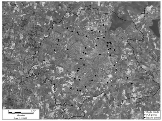
Figure 1.
Ponds owned by VCS Denmark (grey), private ponds (black) and the 12 experimental ponds (white subpool of the grey ponds) in Odense municipality. Contains data from the Danish Agency for Data Supply and Efficiency and VCS. Denmark.
2.2. GIS Analysis
The stormwater ponds were analyzed using the Geographical information systems program MapInfo Professionals version 12.5. MapInfo was used to estimate the surface area (water surface for wet ponds and bottom area for dry ponds), pond type (permanently wet and dry ponds, storage ponds that are only used during heavy rain events (both wet and dry) and ponds that receive wastewater), storage volume and wet volume (in the wet ponds), distance between inlet and outlet, the catchment type and catchment size (total and reduced (the paved fraction). MapInfo layers containing basis information about pond position, type codes, pipe connections and partial catchment areas over individual neighborhoods were kindly supplied by VCS Denmark. These layers were used to determine pond types, ages and catchment distributions and further calculations of ratio between pond volume and the paved catchment area.
2.3. Sampling Water and Sediment
The 12 ponds for detailed examinations were selected based on age and size to gain a diverse collection. From the 12 ponds (10 wet and 2 dry) samples of water, sediment and biodiversity where gathered. Sediment samples were collected using kayak tubes (8 cm diameter). The sediment was sliced in 1 cm intervals and analyzed for dry weight (DW) and OM with double determination. DW was determined by drying the samples at 105 °C for 24 h and OM was determined by loss on ignition (LOI) with a sample of dried sediment being incinerated for 5 h at 520 °C and cooled until constant temperature. TP was measured by transferring 0.1 g combusted sediment, adding 8 mL. 1 M HCl and boiled at 120 °C for 60 min. Absorbance was thereafter measured spectrophotometrically at 880 nm [38]. The detection limit was 15 µg/L. In addition, the metal content in the sediment in the upper 1 cm was measured (Al, Cr, Cd, Pb, Zn, Cu) by transferring 0.2 g dry sediment to test tubes adding 6 mL 65% HNO3, after which the samples were microwaved at 1600 W for 15 min. and lastly measured on ICP-OES (inductively couples’ plasma with optical emission spectroscopy; Optima 2100, Perkin Elmer). Detection limits was 1.0 µgAl/L, 0.1 µgCd/L, 0.2 µgCr/L, 0.4 µgCu/L, 1.0 µgPb/L and 0.2 µgZn/L. TP, DW, OM and metal content was calculated as mg/g DW. In addition, water concentrations of dissolved and particulate substances were measured but is not included in this paper as the sediment contents was chosen as the focus due to the very short retention time in the water phase.
2.4. Biodiversity
All the samples were collected from February to mid-April 2017. In each wet pond two kick samples were collected from both the inlet and outlet area in the ponds. Along the entire pond shoreline nets were used to sample for invertebrates and three samples were collected from the bottom in the middle of the ponds. For the execution of the kick sample the method described in Danish Environmental Agency [39] was utilized. Three sediment cores from the center of each wet pond were collected with kayak tubes (8 cm diameter). The first 5 cm of the cores were sliced in 1 cm intervals and the number of species and animals were determined. The shoreline was screened using a revised version of the pick-samples used for streams and described in [39]. The screening was performed using fishing nets and animals was picked from the stones and plants using tweezers for one turn around the pond without time limit.
The insects in the dry ponds were collected by the use of 7 “drop-traps” in each pond [40], in which a soap mix had been added [41]. The traps were left for 24 h and animals were preserved using 70% ethanol. The pond GA1 has a large dry area (here called GA1-DA) and it was decided to examine this area with regards to biodiversity too.
2.5. Diversity Indexes and Animal Designation
Shannon–wiener index (H’) and Pielou Evenness (J) were calculated based on the number of species (S) and abundance of animals (N). H’ was calculated as [42]:
where Pi is the relative abundance of each species. H’ results in a value between 1.5–3.5. The higher the value, the higher biodiversity is indicated.
J measures the uniformity of a population with a value between 0–1, in which 0 indicates few dominant species and 1 indicates an even number of animals between species. Smith et al. [43] and Pielou [44] methods was followed to calculate J. In this paper, animals’ species will mostly be designated by their order. This is except for the group designated “others”, which comprises of animals found in less than 1% abundance.
2.6. Statistics
To analyze significant differences between the catchment areas a one-way ANOVA was utilized. To analyze and show the impact of ratio and age, different methods was applied. To gain an overview of the 12 experimental ponds in relation to ratio and age a column diagram was chosen. The column diagrams show the ponds arranged from smallest/youngest to largest/oldest pond. The ponds are further subdivided in the ratio categories <250 m3 red·ha−1 and >250 m3 red·ha−1 and age categories 0–5 years, 6–11 years and >11 years. Linear and logarithmic correlations of DW, OM, TP, metals, S, N, H’ and J as functions of ratios and ages were determined for the 12 experimental ponds and tested with a Shapiro–Wilk normality test, but not shown graphically. In order to compare contents in the pond’s inlet and outlet areas a Student’s t-test was utilized to determine possible differences. For the dry ponds the biodiversity and animal distribution were only shown for the catchment types and not included in further statistical analysis or regressions. Statistical analysis was performed in Sigmaplot 13.0 and for all tests a significance level of α = 0.05 was chosen.
3. Results
3.1. A summary of Pond Characteristics
The stormwater ponds were examined with respect to pond types (divided into dry/wet receiving separate stormwater and ponds receiving wastewater), age distribution (age from construction or modification), catchment types and the ratio between pond volume and reduced catchment area (Figure 2). It should be noted that the charts showing catchment types (79 ponds) and ratio (59 ponds) both have fewer ponds compared to pond types and age distribution (135 ponds). Ponds in series connection were excluded from analysis of catchment type and ratio. Regarding ratio, there are even fewer ponds listed as the dry ponds are not included.
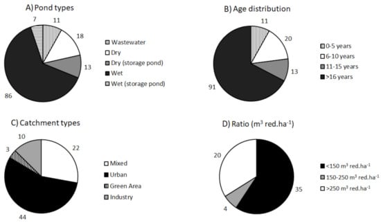
Figure 2.
Stormwater ponds in Odense Municipality sorted into pond types: wet ponds, dry ponds, dry and wet ponds that are used for storage during large rain events (all receive separate stormwater) and ponds that receive wastewater (A). Age distribution: The age of the ponds is distributed in the intervals 0–5 years, 5–10 years, 10–15 years, >16 years (B). Catchment types: The catchment types of the ponds are distributed by the types urban, industry, mixed and green areas (C). Ratio is distributed between the intervals <150 m3 red·ha−1, 150–250 m3 red·ha−1 and >250 m3 red·ha−1 (D).
Most of the ponds, 86 of 135 ponds, are wet ponds followed by dry ponds (18 ponds), dry storage ponds (13 ponds), ponds receiving wastewater (11 ponds) and the least common pond type is wet storage ponds (7 ponds). When examining the age distribution, it becomes apparent that most of the ponds are quite old with 91 of the 135 ponds being above 16 years old. There are 13 ponds in the interval 11–15 years, after which there are 20 ponds in the age interval 6–10 years and only 11 ponds are between 0–5 years old. The catchment type distribution shows that most of the ponds (44) receive water from an urban catchment area. After the urban catchment the most common catchment type is the mixed catchments (22 ponds). The industrial and green area catchments have only 10 and 3 ponds, respectively. Regarding the pond ratio (volume to impervious catchment area) a majority of the ponds are quite small compared to their catchment; thus, 35 ponds have a ratio < 150 m3 red·ha−1. There are only 4 ponds in the interval 150–250 m3 red·ha−1 and the remaining 20 ponds have a ratio >250 m3 red·ha−1. To determine whether the ponds in the different catchment types differ significantly from one another, a range of parameters was determined for each pond (Table 1).

Table 1.
Characteristics of all ponds: The four catchment types with corresponding average age (years), average surface or bottom area (m2), average ratio and average distance from inlet to outlet (m). All parameters are shown with ranges (incl. min-max) and standard deviation (SD). Ponds in series connections is excluded. Selected experimental ponds: The four catchment types with average and ranges (incl. min-max) of age (years), pond surface- or bottom area (m2), volume (m3), ratio and distance from inlet to outlet (m).
Ponds in the industrial and mixed areas had similar age ranges with, respectively, 27 years (ranging from 5–57 years) and 23 years in average (ranging from 5–54 years). The urban ponds were on average older than the mixed and industrial ponds with an average age of 31 years, but a comparable range of 2–58 years. The ponds in the green areas were the youngest with an average age of 17 and a smaller range of 2–44 years. Concerning the surface/bottom area of the ponds the green ponds are the largest with an average of 16,712 m2, ranging from 49–46,609 m2. The green ponds are followed by the mixed and industrial ponds with similar average sizes of 1618 m2 and 1974 m2, respectively. The mixed and industrial ponds have very different ranges though, with the industrial ponds having the lowest range of 131–5709 m2 and mixed with the largest range of 16–17,701 m2. The urban ponds are the smallest with an average of 1159 m2, but with a rather large range of 10–11,558 m2. For ratio and distance between inlet and outlet the green ponds are the largest with an average ratio of 2234 m3 red·ha−1 and a distance of 157 m. Urban and mixed ponds have a similar ratio of 361 m3 red·ha−1 on average and the industrial ponds are the smallest with a ratio of 290 m3 red·ha−1. The urban and industrial ponds have similar lengths from inlet to outlet-49 and 45 m, respectively, while the mixed ponds have the shortest distance of 37 m. There were found to be no significant differences between pond age in the different catchment types, but significant differences were found between the ponds in the green areas and the other catchment types with respect to water surface/bottom area, ratio and distance between inlet to outlet (Table 2).
Table 2.
Oneway-ANOVA test of differences between the catchments area industry, urban, mixed and green areas for the parameters Bottom/surface area (m2), ratio (m3 red·ha−1) and distance from inlet to outlet (m). Diff of means and p-value incl.
3.2. The 12 Experimental Ponds
The 12 selected ponds vary in age and size (Table 1). The ponds in urban, mixed and green areas are on average 18 years and range from 2–34 years). Though the range is a bit larger for the ponds in the mixed areas (6–50 years). The industrial ponds are younger with an average age of 6 years and a range of 5–7 years. The ponds in the green areas are the largest both regarding surface/bottom area and volume with an average of 24,035 m2 and 23,756 m3, respectively. The urban, industry and mixed ponds have similar surface areas of 3462 to 3770 m2 on average. The ratio is highest for the mixed areas with an average ratio of 3005 m3 red·ha−1, followed by the ponds in the green areas with an average of 1756 m3 red·ha−1. The urban and industrial ponds are the smallest with averages of 657 m3 red·ha−1 and 169 m3 red·ha−1, respectively.
Regarding the distance from the inlet to outlet the ponds in green areas have the largest distance with an average of 130 m, followed by the urban ponds, the mixed and industrial with an average length of 118, 83 and 53 m, respectively.
The 12 selected ponds are generally larger compared to the average of the municipal ponds, especially the mixed and urban ponds have a larger ratio (46–88% larger) and greater distance, 56–59%, from the inlet to outlet. Age fits somewhat with the municipal averages, except for the industrial ponds which are newer. In almost all cases (except for ratio and distance from inlet to outlet for the mixed ponds), all values fall withing the SD value. It is therefore concluded that these ponds are decent representatives for the conditions in the different catchments for Odense municipality.
3.2.1. DW, OM and TP
Catchment Classification
When displaying DW (%), OM (mg OM/g DW) and TP (mg TP/g DW) and classifying the ponds after catchment types, differences between the ponds were observed. These differences are shown in Table 3, but only for the inlet areas as the outlets did not yield any significant differences. The DW in the inlet areas tend to be higher in the urban and green ponds compared to the industrial and mixed ponds. For 3 of the 4 urban ponds (Ur2, Ur3 and Ur4) the average DW was 76.2% (69.8% if Ur1 is included) compared to an average DW in the industrial and mixed ponds of 41.8% and 50%, respectively. The green ponds were close to the values of the urban ponds with an average of 73.3%. These differences in inlet area DW, however, were not significant (Table 3). DW in the outlet areas were generally lower than in the inlet areas. The DW was on average 38% in the outlet areas of the urban ponds, while the corresponding DW was 43–48% in the remaining ponds. These differences between the inlet and outlet area were significant (p = 0.019) (Figure 3A, Table 4). For OM, there was a tendency for industrial and mixed ponds to have a higher OM content in the inlet area compared to the content in the inlet areas of urban and green ponds. The average OM content in the inlet area for industrial and mixed ponds were 117 mg OM/g DW, while in the urban and green ponds it was 37 mg/g DW and 29 mg/g DW, respectively. OM in the outlet area was generally higher compared to the content in the inlet areas with the urban and green ponds having the highest average content of 135 mg OM/g DW and 122 mg OM/g DW, respectively. In the industrial and mixed ponds, the average outlet area content was 107 mg OM/g DW and 94 mg OM/g DW. There was a significant difference between the OM content in the inlet- and outlet areas for the urban ponds (p = 0.022) (Figure 3A, Table 4). TP tend to be higher in the industrial and mixed ponds compared to the urban and green ponds. The average TP content in industrial and mixed ponds were 1.2 and 1.0 mg TP/g DW, respectively, while the urban and green ponds had, on average, lower contents of 0.4 and 0.6 mg TP/g DW, respectively. This difference in TP contents in the inlet area was significant, with higher TP in industrial ponds compared to urban (p = 0.009) and green ponds (p = 0.041). The mixed ponds had a significantly higher TP content in the inlet area compared to the urban ponds (p = 0.009) and showed the same tendency compared to the green area ponds (p = 0.064) (Table 3). Concerning the outlet area, the TP content was similar for all catchment types with values between 0.9–1.3 mg TP/g DW with the mixed ponds having the highest content (Table 4). A significant difference between the TP content in inlet and outlet areas in the urban ponds (p = 0.029) was found (Figure 3A, Table 4).
Table 3.
One-way ANOVA test of differences in DW and metal content (Zn, Cu, Cr and Pb) in inlet areas versus catchment types industry, urban, mixed and green areas.
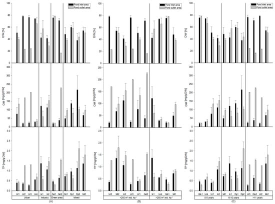
Figure 3.
DW (top), OM (middle) and TP (bottom) in the sediment (mg/g DW) in the ponds inlet and outlet areas classified by the catchment areas: Urban, industry, green areas and mixed (A), volume to impermeable catchment area ratio in the intervals <250 m3 red·ha−1 of >250 m3 red·ha−1 (B) and age in the intervals 0–5 years, 6–11 years and >11 years (C) with SEM.
Table 4.
Results of a Student’s t-test between the DW [%], OM, TP [mg/g DW], Al, Zn, Cu, Cr, Cd and Pb [mg/g DW] content in the inlet and outlet compared.
Effect of Pond Volume Versus Impermeable Catchment Area
DW, OM and TP content in the sediment are partly affected by the ratio of volume versus catchment area. The DW in the inlet and outlet areas showed different tendencies. The inlet area DW does not seem to change with increasing ratio (on average 62% DW for ponds <250 m3 red·ha−1 and 60% for ponds >250 m3 red·ha−1). DW in the outlet area tend to increase with higher ratio, with on average 30% DW for ponds <250 m3 red·ha−1 and DW and 60% for ponds >250 m3 red·ha−1. This notion of higher DW with higher ratio in the outlet area was close to being significant (p = 0.052).
OM in the inlet areas did not change with increasing ratio. However, a strong tendency for lower OM in the outlet areas with higher ratio was observed. OM in the outlet area was lower for the ponds <250 m3 red·ha−1 (average 163 mg OM/g DW) compared to the ponds with ratio >250 m3 red·ha−1 (average 52 mg OM/g DW). This was a significant logarithmic correlation (p = 0.033).
In the outlet areas TP showed a tendency to be negatively correlated to higher ratio. The average TP in the outlet area decreased from 1.3 mg TP/g DW for <250 m3 red·ha−1 to 0.6 mg TP/g DW for >250 m3 red·ha−1. This showed to be a significant logarithmic correlation (p = 0.037). No such tendency was observed for the inlet area which had similar averages for <250 m3 red·ha−1 and >250 m3 red·ha−1 of 0.7–0.8 mg TP/g DW (Figure 3B).
Impact of Pond Age
The DW, OM and TP sediment content was increasing with age. For 3 of the 4 oldest ponds a large difference in DW between the inlet and outlet areas were observed in the ponds. DW for the inlet area averaged 70% and the outlet area averaged 28%. For the ponds in age interval 0–5 years the DW in the inlet area was on average higher compared to the outlet, with an average DW of 60% in the inlet areas and average DW of 53% for the pond’s outlet area. For the ponds in the 6–10 years interval, it was roughly the same average DW for both the inlet and outlet areas (47–49%). This tendency towards lower DW content in the outlet areas with higher age was a significant logarithmic correlation (p = 0.024). OM did not show such tendency in the inlet area, but a similar tendency towards higher OM with higher age in the outlet areas. Average OM for the ponds <10 years was 85 mg/g DW which increased to 173 mg/g DW for the ponds >11 years. This tendency towards higher OM in the outlet area with higher age was a significant logarithmic correlation (p = 0.014). A similar tendency for TP in the pond’s outlet areas was found. TP in the outlet areas increased from 0.7 mg TP/g DW (0–5 years) to 1.0 mg TP/g DW (6–10 years) and 1.5 mg TP/g DW for ponds >11 years (Figure 3C). This tendency towards higher TP in the outlet areas with higher age was a significant logarithmic correlation (p = 0.026).
3.2.2. Metals
Effect on Metal Content by Catchment Type
Tendencies of different metal content in the ponds with different catchment areas was shown when classifying the ponds after catchment types (Figure 4A). In the urban ponds, there was a higher Al content in the outlet area compared to the inlet area for three of the ponds. The outlet area of these ponds had an average Al content of 16 mg Al/g DW compared to 9 mg Al/g DW in the inlet area. In addition, the mixed ponds had an inlet area average Al content 9 mg Al/g DW, compared to the industrial and green area ponds with 8 and 2 mg Al/g DW, respectively. Concerning the outlet area, the industrial and mixed ponds had an Al content of 7 mg Al/g DW and 8 mg Al/g DW, respectively, whereas the ponds in green areas only had on average 3 mg Al/g DW. Though not statistically significant (p = 0.074), a strong tendency was observed towards higher Al contents in the outlet area of urban ponds compared to the inlet area (Table 4).
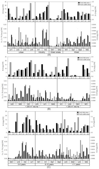
Figure 4.
Al, Zn, Cu, Cr, Cd and Pb (mg/g DW) content from the ponds inlet and outlet areas classified by the catchment types urban, industry, green areas and mixed (A), ratio intervals (<250 m3 red·ha−1 and >250 m3 red·ha−1) (B) and age in the intervals 0–5 years, 6–10 years and >11 years (C).
In addition, significant differences in Zn content between ponds with different catchment areas were found. There was a tendency of the Zn content being higher in the industrial ponds compared to the urban-, green area- and mixed ponds. The industrial ponds had an average Zn content of 1.06 mg Zn/g DW in inlet area and 0.97 mg Zn/g DW in the outlet area. Following the mixed ponds had an inlet area content of 0.57 mg Zn/g DW and an outlet area content of 0.49 mg Zn/g DW. In the urban ponds the average inlet area Zn content was 0.23 mg Zn/g DW and a bit higher in the outlet area (0.32 mg Zn/g DW). The green area ponds inlet area contents were generally lower compared to the other ponds, with an average of 0.09 mg Zn/g DW. The outlet area of the pond GA1 had the lowest Zn content, of all the ponds (0.008 mg Zn/g DW). The industrial ponds had a significantly higher Zn-content in the inlet area compared other catchment types (p = 0.0026 versus urban ponds, p = 0.029 versus green areas) (Table 3).
For the metals Cu, Cr, Cd, Pb there seem to be differences in the content based on the catchment types. The most notable difference was found in the inlet area of industrial ponds with Cu, Cr and Pb contents, being higher compared to the other ponds. The average content in inlet areas of the industrial ponds were 0.14 mg Cu/g DW, 0.06 mg Cr/g DW and 0.05 mg Pb/g DW, while the collective average inlet area content for the remaining ponds were 0.04 mg Cu/g DW, 0.02 mg Cr/g DW and 0.03 mg Pb/g DW. There was a significant difference concerning Cu between the industrial ponds and the ponds with other catchment types (Table 2).
For 3 of the urban ponds there was a higher content of Cu, Cr and Cd in the pond’s outlet area (0.06 mg Cu/g DW, 0.04 mg Cr/g DW, 0.002 mg Cd/g DW and 0.10 mg Pb/g DW) compared to the inlet area (0.02 mg Cu/g DW, 0.01 mg Cr/g DW, 0.001 mg Cd/g DW and 0.03 mg Pb/g DW), though this turned out not to be a significant difference. There were no significant differences concerning metal contents in the outlet area and different catchment types (Table 4).
Ratio Impact on Metals Contents
Metal content in the sediment tends to be affected by the ratio between the ponds volume and the impervious catchment area (Figure 4B). Aluminum content in the ponds with a ratio <250 m3 red·ha−1 was higher in the outlet area (11 mg Al/g DW) compared to the inlet area (7 mg Al/g DW), but in the ponds with a ratio >250 m3 red·ha−1 there was no difference between the average Al content in the inlet area (9 mg Al/g DW) and outlet area (9 mg Al/g DW). For Zn a slightly lower content in the outlet area with higher ratio was observed, with an average of 0.20 mg Zn/g DW less Zn in the outlet area compared to the inlet area, however, not a significant decrease (p = 0.143). For Cu, Cr and Pb there was an overall tendency towards a higher metal content in the ponds with ratio <250 m3 red·ha−1 in the inlet area with a difference of 0.03 mg Cu/g DW, 0.01 mg Cr/g DW, 0.0006 mg Cd/g DW and 0.02 mg Pb/g DW) and the outlet area (0.07 mg Cu/g DW, 0.03 mg Cr/g DW, 0.0013 mg Cd/g DW and 0.04 mg Pb/g DW), but no significant differences between the inlet and outlet area contents in neither category were observed. Especially the Cu and Cr contents in the outlet shows a tendency towards a lower content with a higher ratio (logarithmic decrease). However, no significant correlation was observed for neither Cu (p = 0.086) or Cr (p = 0.148). For Cd and Pb there was a strong tendency towards a lower content in the ponds with a higher ratio. Especially in the outlet area which showed a significant logarithmic decrease for Cd (p = 0.034) and an almost significant logarithmic decrease for Pb (p = 0.097).
Impact of Pond Age on Metals Content
The metals content tends to increase with higher pond age, with 3 of the 4 ponds >11 years having vastly higher metal contents in the outlet area compared to the inlet areas (Figure 4C). These three old ponds (Ur3, Ga2 and Ur2) had Al and Zn contents in the outlet area which was 10 mg Al/g DW and 0.45 mg Zn/g DW higher than the inlet area content. Copper, Cr, Cd and Pb content in the outlet areas was also higher than the inlet area contents with, respectively, 0.064 mg Cu/g DW, 0.027 mg Cr/g DW, 0.0014 mg Cd/g DW and 0.078 mg Pb/g DW, but not significantly. For Pb, there was a strong tendency towards a higher Pb content in the outlet areas compared to the inlet areas with higher age. The Pb-content in the outlet areas increased logarithmically with age, though not significantly (p = 0.07), but a strong tendency. This correlation is assumed to be due to Denmark’s previous use of leaded gasoline [45].
3.2.3. Biodiversity
Water Phase
Catchment classification:
S, N, H’ and J were determined for 10 wet ponds and 2 dry ponds (Figure 5A). For the wet ponds, this part only consists of the species found in the water phase, while for the dry ponds, it is the total number of species. For 6 of the 10 wet ponds, there was found a higher number of S in the inlet area compared to the outlet area.
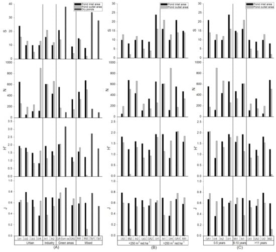
Figure 5.
S (top), N (top-middle), H’ (middle-bottom) and J (bottom) in the inlet and outlet water phase for wet ponds and collectively for dry ponds, classified by the catchment areas: Urban, industry, green areas and mixed (A), ratio (m3 red·ha−1) in the intervals <250 m3 red·ha−1 of >250 m3 red·ha−1 (B) and age in the intervals 0–5 years, 6–11 years and >11 years (C).
S, N, H’ and J were similar for all inlet areas with an average of 12–14 species. The dry ponds had a higher number of species with 38 species in GA1 and on average 31 species in Dp1 and Dp2. Most individuals were found in the industrial and mixed ponds with an average of 524 and 574 N, respectively, followed by the green ponds (447 N) and fewest individuals were found in the urban ponds (237). The dry ponds had fewer individual animals compared to the wet ponds with 100 individuals in GA1 and an average of 128 in Dp1 and Dp2. H’ was on average highest for the industrial ponds with 1.8, followed by the green area ponds (1.6), urban (1.5) and mixed (1.4). The dry ponds had a higher H’ than the wet ponds with 3.2 for GA1 and a lower average for the mixed Dp1 and Dp2 (2.3). J was highest for the industrial ponds with 0.7, whereas the other ponds had an average of 0.6. The dry ponds had J comparable to the wet ponds, although a bit higher with 0.9 for GA1, which was the highest J measured for any of the ponds. For the dry mixed ponds, the average J was 0.7, which is still in the high end. The conditions in the outlet areas of urban ponds were similar to the inlet area with S = 12, but more individuals (398 N) and H’ and J was the same as the inlet area with 1.5 (H’) and 0.6 (J). For the industrial ponds S and N were both overall higher (S = 17 and N = 635), but H’ and J were lower (H’ = 1.2 and J = 0.5). The green ponds had lower S and N in the outlet area compared to the inlet area (S = 9 and N = 194), but with similar H’ and J of 1.5 and 0.7, respectively. All values were lower for the mixed ponds outlet areas with S = 8, N = 422, H’ = 1.0 and J = 0.4 (Figure 5A). Despite the described differences in S, N, H’ and J between the inlet and outlet areas, no significant differences were found.
Ratio impact on biodiversity:
In general, fewer species were found in the ponds <250 m3 red·ha−1 both concerning inlet area (12 S) and outlet area (9 S), while for ponds with a ratio >250 m3 red·ha−1 S was on average 16 both for inlet and outlet areas (Figure 5B). There was a logarithmic tendency towards higher S with higher ratio for both inlet and outlet areas. A higher N was found in ponds with ratio <250 m3 red·ha−1 both in the inlet (441 N) and outlet area (506 N) compared to the ponds with ratios >250 m3 red·ha−1 which on average had 379 N in the inlet area and 335 N in the outlet area, but no significant tendency. For H’, there was not found any changes with ratio in the inlet areas and the average H’ was 1.6 for both ratio categories. H’ for the outlet areas tend to be lower for the <250 m3 red·ha−1 with an average of 1.1, compared to the ponds with >250 m3 red·ha−1 with on average 1.7. This tendency of higher H’ in the outlet area with higher ratio was a logarithmic correlation close to significant with p = 0.06. For J no correlations neither at inlet nor outlet were observed.
Impact of age
There was a clear tendency towards lower numbers of animal species in both the inlet and outlet areas with age (Figure 5C). At the inlet area the average number of species for 0–5 year and 6–10 year old ponds were 16 S, but the average dropped to 9 species for the ponds >11 years old. For the outlet area the average number of species for 0–5 years and 6–10 years was similar with 14 S and 18 S, respectively, but like for the inlet area, the average dropped to 6 species for the ponds >11 years old. Lower numbers of species with increased age were significant both at the inlet area (p = 0.04) and at the outlet area (p = 0.006). There was also a tendency towards fewer individuals with increasing age. For both the inlet and outlet the average number of individuals was about 500 for 0–5 year and 6–10 year old ponds, but dropped below 300 individuals for >11 year old ponds, but not significant correlations. The decreasing tendency with age seen for S and N was also the case for H’, though more pronounced at the outlet than the inlet. At the inlet the average H’ for 0–5 year and 6–10 year old ponds were 1.6 and 1.8, respectively, but decreased to 1.4 for the >11 years ponds. As mentioned, this tendency was much more prominent at the outlet which had an H’ for 0–5 year and 6–10 year old ponds of 1.7 and 1.5, respectively, which decreased drastically to 0.9 for the >11 years ponds. This decrease seen in the outlet was significant (p = 0.01). The decreasing biodiversity with age was not as prominent for J. At the inlet the average J was 0.6 across all age intervals. The tendency was a little stronger with decreasing J against age at the outlet which dropped to 0.5 from 0.6 for ponds >6 years (Figure 5C).
Correlations between water phase biodiversity and DW, OM, TP and metals.
Linear and logarithmic regression between the water phase biodiversity (dry ponds not included) and sediment content of DW (%), organic content and TP yielded different results for the inlet and outlet. In the inlet area, N was the only factor affected. N decreased versus increasing DW (p = 0.026) but increased in response to higher organic content (p = 0.03). N also increased in response to higher TP (p = 0.07), though not significantly. In the outlet area S and H’ as a function of TP decreased with increasing TP-content significantly (p = 0.006 (S) and p = 0.007 (H’)). S, N, H’ and J in the inlet and outlet were also tested versus the sediment metal content. None of the correlations were significant for the inlet area, but H’ decreased logarithmically with increasing metal contents of Zn (p = 0.03) and Cu (p = 0.08) in the outlet area.
Sediment
The largest number of different species were found in the ponds with mixed catchments (seven species), followed by the ponds with urban catchments (two to five species). The ponds with green catchment areas had three to four species and the industrial ponds had the lowest S with only one to two species (Figure 6).
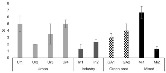
Figure 6.
S in sediment categorized after the catchment types urban, industry, green area and mixed without dry ponds.
Distribution of Species in Water Phase
It was varied which animals were the most common in the ponds with different catchment areas, when looking at the animal distribution at the inlet and outlet area collectively (Figure 7). Haplotaxida, primarily with species of naididae and tubificidae, was found in all the ponds. Haplotaxida was the most dominant family descending in the order of mixed (67%) >> industrial (55%) > urban (21%). For Green areas, haplotaxida was also the dominant family (50%), but for the pond GM1 the species Chaotogaster diaphamus did comprise 15% of the collected haplotaxida. Diptera was also found in all catchment types in descending order of industrial (20%) >> urban(17%) > green areas (15%) > mixed (15%). Cyclopoida was found in descending order in the catchments urban (33%) >> mixed (11%) > industry (9%). Isopoda was found in much smaller quantities in urban (2%) >> green areas (2%)> industry (1%). Cladocera was found in mixed (5%) and industry (1%), crustacea in urban (3%) and industry (3%), lumbriculida in urban (2%) and industry (2%). Ephemeroptera was only found in urban (5%) and green areas (1%). Some animals were found exclusively in one catchment type. Diplostraca was only found in the urban catchment (13%). The animals of amphipoda (3%), hydroida (3%), nematoda (2%), pulmonata (20%) and trichoptera (1%) was only found in the green areas. Lastly, sphaeriida (3%) and hemiptera (1%) were found only in the industrial ponds.
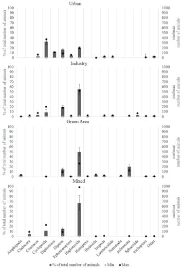
Figure 7.
Invertebrate distribution (%) of total number of animals found in inlet- and outlet areas collectively of each catchment area. With indication of the maximum and minimum number of animals found with standard deviation.
Correlations between Biodiversity and Ratio, Age, DW, Organic Content, TP and Metals
The linear regression analysis between S versus ratio and age gave for ratio a significant relation (p = 0.04), while the relation with age was not significant (p = 0.88). Linear regression between S, H’ and J versus DW (%) and organic content and TP (mg/g DW) yielded quite different results. For S, H’ and J versus DW (%) there were no correlations, while S as a function of organic content showed a tendency towards decreasing S with increasing organic content; however, this was not significant (p = 0.300). For S, H’ and J as a function of TP all parameters decreased with increasing TP-content and very close to significant (p = 0.09 (S), p = 0.07 (H’) and p = 0.05 (J). S, N, H’ and J were also tested versus the sediment metal content. None of the correlations were significant, but S and H’ tend to decrease linearly with increasing metal content, except for Al which showed the opposite trend, but not significantly. S decreased linearly with increasing Cu and H’ decreased logarithmically with increasing Cu and Zn. J also decreased logarithmically with increasing Cu and Zn.
4. Discussion
4.1. Summary of Pond Characteristics
The expected prevalent presence of ponds with urban and mixed catchments was confirmed by the order urban >> mixed > industrial > green. As the study was conducted in the Odense municipality and most of the ponds are placed outside the city center, this was expected. There are only few ponds in the central city, due to the common sewer systems in the older city parts. The summary revealed that a majority of the ponds have a ratio below 150 m3 red·ha−1 and an age above 16 years since construction. This result illustrates, as expected, that many of the ponds are old because stormwater ponds have been considered BAT for decades. However, it also illustrates another tendency: many ponds were, especially earlier, designed too small to ensure a sufficient retention time for effective settling of particles. This can potentially increase the risk of insufficient removal of pollutants in the ponds. However, it is more recent that pollutant removal has been prioritized too and where a ratio of >250 m3 red·ha−1 is necessary for sufficient settling. Many stormwater ponds were originally built exclusively to store and delay stormwater during rain events for hydraulic reasons. Therefore, it was not necessary to build them larger at that time. Nevertheless, with the new expectations to both storage and treatment, many existing ponds are too small. When comparing ponds in different catchment areas, no significant differences with regards to age and distance from pond inlet to outlet were observed and only the ponds in the green areas were significantly different with regards to surface/bottom area and ratio. However, the significant difference between the ponds in green areas and the other ponds are not indicative for several reasons, but mainly because of pond GM1. Pond GM1, also referred to as “Lake Glisholm”, is an enormous stormwater pond with a surface area of 46,609 m2 and the capacity to store 87,000 m3 of stormwater [46]. It was built as a mitigating measure to limit hydraulic effects on stream Lindved and avoid flooding [46,47]. At the time of examination GM1 only received diffuse runoff from the catchment area which largely constitutes uncultivated area and the pond was filled with groundwater and surface runoff. However, this is changing as the catchment area is developing and all the impermeable areas are established. Then, the catchment type will change to “industrial” when construction completes.
In conclusion, the catchment type is evidently not considered when designing the ponds.
4.2. Experimental Ponds
4.2.1. Catchment Types
The inlet- and outlet areas in the urban ponds follow opposite trends with minerogenic sediment in the inlet area and organogenic sediment in the outlet area. The significantly higher DW content in the inlet area could indicate that more or larger particles washed out from the catchments are settling there. These particles most likely stem from road/pavement surfaces and the OM is most likely plant material that washed off the surfaces during rain events. It might also indicate that storm events cause resuspension in the inlet pond areas, flushing smaller particles and organic materials to the outlet area and leaving the heaviest particles. This could be remedied by further reducing the water velocity when entering the pond, such as implementing large rocks or other obstacles [47,48]. Industrial and mixed ponds had higher TP contents in the sediments compared to urban and green areas and significantly higher content in the outlet area. This is expected as smaller particles and organic content accumulates in the ponds’ outlet areas and P is often bound to small particles. This corresponds with our hypothesis that higher contents of pollutants might be found in ponds with industrial and mixed catchments, because higher contents of metals and TP are often found in areas most affected by human activities-such as industrial complexes and roads with heavy traffic. Egemose et al. [19] and Göbel et al. [21] had similar findings. The metals content indicated the same trend with the industrial ponds being most heavily affected by the metals Zn and Cu, but not with a significantly different content between inlet and outlet areas.
For Al there was also a tendency towards higher outlet area content compared to the pond inlet areas, which seem to be most prevalent for the urban catchments. The high content might be due to aluminum being one of the most commonly used metals in Denmark (ex. vehicles, packaging, construction) and is also naturally found in the ground [49,50]. Aluminum and other metals will degrade over time and be deposited on to roads and other surfaces at which point it can be washed into the ponds. The tendency towards higher content in the outlet area might indicate that metals are not settling equally in the whole pond and/or are accumulating or being flushed towards the pond’s outlet area due to insufficient retention time. Aluminum may be bound to clay particles, which are very small/light and would require a long residence time to settle and this makes resuspension very likely to occur [49].
The industrial and mixed ponds tend to have higher metal, OM and TP contents in the outlet area, even with ratios > 250 m3 red·ha−1. This increases the risk of flushing pollutants from the ponds during large and intensive events. A suggestion could be to increase the retention time by prolonging the water distance through the ponds. This might be done by introducing more obstacles in the ponds such as small islands or large rocks, especially in the inlet area. Installing a baffle that will act as a physical barrier between the pond inlet and outlet areas is also an option. The baffle forces the water through, above or around the barrier and further increases the residence time [48]. Lake Glisholm is an example of a stormwater pond in which a baffle between the inlet area and the rest of the pond has been installed [46]. It would also be prudent to ensure a depth of 1 m to maintain the planned ratio and residence time and lower the resuspension risk. Ponds get filled with sediment due to settling of particles over time, which reduces the residence time and the originally designed ratio.
4.2.2. Ratio and Age
The outlet area contents of DW showed a tendency to increase with higher ratio, while OM and TP decreased significantly with higher ratio in the outlet area. The same significant correlations were not found for the metals, but some trends were observed. Outlet area content of Zn support the previous findings of Egemose et al. [19] and Mallin et al. [51], who showed a metal content drop with higher ratio, though not significantly in this study. The metals Cu, Cr, Cd and Pb also showed the expected content decrease with increasing ratio, which was significant for Cd. Egemose et al. [19] found contents that were a bit lower but close to the contents found in this study. Zinc loads especially were much higher for several ponds in Odense. Egemose et al. [19] examined ponds in Aabenraa in the Danish region of Southern Jutland which has a population density approx. ten times lower than that of Odense. This could indicate that the general metal load from the catchment is higher in Odense compared to Aabenraa. These lower contents of particles and pollutants in the outlet areas of the ponds with higher ratios confirm our hypothesis and is assumed to be because of the comparably greater volume in the ponds for dispersion of incoming particles. This also results in a longer residence time and, thus, higher chance of small particles to settle in the pond instead of accumulating in the outlet area.
Metals are often bound to particles <63 µm, which might be why there was an observed tendency of Zn, Cu, Cd and Pb contents being higher in the outlet areas of older ponds. Lead showed the strongest tendency to increase with age. This might be explained by the 3 ponds Ur3, Ga2 and Ur2 that are 34 to 50 years old. These ponds were, thus, constructed and in use, while leaded gasoline was still in use in Denmark. Lead-fuel was banned in 1994 [45] but because these ponds have accumulated sediment during their entire lifetime, it is stipulated that this Pb-content is the remnants of this former practice. This paper did not demonstrate any significant correlation between age and metal contents, possibly due to the low number of examined ponds. Egemose et al. [19] did however, find such a trend. This tendency of pollutant accumulation in the outlet areas with age might be explained by a limited retention potential. Sønderup et al. [18] demonstrated a significant decrease in retention (%) over time due to buildup of particles through sedimentation, which may in turn lead to increased resuspension. Because TP, OM and metals are often bound to very small particles they are more likely to be flushed to the outlet area and risk flushing out from the ponds. This could potentially affect downstream ecosystems negatively.
Other communities might also be affected. The effect of stormwater discharge on the microbial community is not a well examined area, but several papers have concluded that surface water pollution can lead to shifts in the microbial community [27,52,53,54]. A previous study has demonstrated that ponds used for raising grass carps (Ctenopharyngodon Idella) can have varying bacterial abundance in response to temperature and oxygen availability [55]. It is likely that the same is the case for stormwater ponds though not many studies have been made on the bacterial abundance or composition in stormwater ponds per se. Studies have indicated that stormwater ponds are not efficient in retaining bacteria, in particular those related to fecal matter, showing at most a 23% removal efficiency [56]. This was stipulated to be due to these bacteria often being bound to fine particles, such as TP, OM and metals can be, which likewise need a long residence time to settle [57]. This is another reason why a proper ratio between the reduced catchment area and wet volume is needed for the ponds to fulfill their purpose of protecting the downstream environment. However, it is an area that requires further study. Sønderup et al. [18] and Egemose et al. [19] concluded that separately high age and low ratio limits retention of nutrients, organic content and metals and in this study it is most likely the combined effects of low ratio and high age.
4.3. Biodiversity
4.3.1. Impact of Ratio and Age on Biodiversity in Water Phase and Sediment
S and H’ increased with higher ratio, but only significantly for S in the sediment. This was expected as a larger ratio could mean more niches, but also, as previously shown, a decrease of pollutants. Mackintosh et al. [58] made a similar correlation and found a negative correlation between S and total catchment imperviousness. It was hypothesized that this correlation might be due to the chemical and physical stress urbanized catchment can induce upon a wetland, meaning fewer species and the domination of the invertebrate population by more pollution tolerant species [59]. Mackintosh et al. [58] found a domination of the more tolerant species compared to the more sensitive ones. In our study the effect of age on biodiversity was very different, both from the observed effect of ratio and between the water phase and sediment.
For S, there was a significant decrease with age for both inlet and outlet areas. For H’, a significant decrease in the outlet area was also observed. This might be due to the observed increase in metals, TP and OM with age and the tendency towards decreasing biodiversity in relation to it. This might also explain the lack of animals in the water phase.
However, the sediment biodiversity is unaffected by age. The same tendency as for the water phase was expected for the sediment. That this was not the case might indicate that even though there are negative effects that can be related to age since construction, this does not ultimately affect biodiversity. Sun et al. [60] had similar findings and concluded that pond age has a relatively low impact on the biodiversity. Invertebrate life is quite versatile and it is likely that this change in the ecosystem happens slowly enough to ensure, that the animals have time to adapt, or that the toxicity levels do not affect the lifespan or reproduction of the animals. Many of the invertebrates found in the sediment (regardless of pond age) were already well adapted to anoxic events and high toxicity (tolerant species), which will be discussed more in the next section.
As previously shown, TP and OM decrease with higher ratio and the same tendency towards S, H’ and J decreasing with higher TP in the sediment was also found. S also decreased with higher OM, while H’ and J were unaffected. Higher TP and OM likely gives rise to anoxic episodes because TP can cause algae blooms and OM requires oxygen for decomposition, making it difficult for invertebrates that are not anoxic tolerant species to survive. S and H’ for the water phase was also tested with respect to TP and found to be decreasing with increasing TP content. N increased with TP though. This indicate that the sediment pollutant contents are not restricted just to the bottom surface, but translate to the water phase too. The higher N indicates this too, because when a higher N (>500 individuals) was observed it was mostly haplotaxida worms (tubificidae and naididae) and diptera larvae (Chironomidae) that were found and these animals are well suited to anoxic environments.
Some metals are known to have a toxic effect on living organisms, such as Cu and Zn. In this study, the sediment content of Cu and Zn tend to affect the biodiversity in the sediment and water phase negatively. Cu and Zn have similar toxic effects on aquatic invertebrates, e.g., limiting growth rates, swimming speed, food consumption, breathing, reproduction and survival [61,62]. The significantly higher Cu and Zn content in the industrial ponds and the lower biodiversity in their sediments (Figure 7) indicates a link: the industrial ponds are most heavily polluted with metals, which negatively affects the biodiversity, though we found no significant correlation. A high metal content does not necessarily mean a worsening of conditions for biodiversity though, it depends on which metal is present and in which concentration. Aluminum showed the opposite trend for the sediment. With higher Al a higher number of species was found, though it did not translate to the water phase. Aluminum has been known to cause respiratory difficulties in fish, but it is an uncommon effect in invertebrates. Furthermore, aquatic invertebrates are generally known for being resistant to damaging effects of Al [50] and Al is only toxic as dissolved forms. Aluminum is not directly having a positive effect on the invertebrates. It is stipulated that it is Al’s binding effect on P in the sediment that can prevent algae blooms in the ponds [63] and, thus, benefit the invertebrates.
This indicates that the pond ecosystems and, thus, biodiversity, is affected by the service they provide in storing pollutants and that it does affect the ecosystem. Sun et al. [60], however, did not find the same tendencies of declining biodiversity with higher pollution levels and concluded that there was no evidence to support the notion of increased pollution levels necessarily limiting biodiversity when looking at number of taxa or Shannon index. However, they measured in the water column not the sediment, while this study indicate there might be a correlation for the sediment, but ultimately it is a subject that requires more research. It is also extremely important to remember that the ponds are technical facilities that are established to protect the nature, environment and biodiversity in the recipients. In addition, that stormwater ponds may be used as substitute ecosystems in cities, but maintenance is extremely important to ensure a constantly high and sufficient functionality concerning both treatment efficiency and habitat [64]. A solution could be to excavate the soil when the biodiversity becomes too uniform (consisting of mainly worms and mosquito larvae) in order to let the more sensitive species repopulate the ponds again. This would allow for a higher biodiversity in intervals or continuously depending on the excavation frequency. Recent studies on a variety of new and reestablished Danish lakes, several of which resembling large stormwater ponds in form and function, have reached similar conclusions [65,66]. Shortly after their establishment, the new lakes exhibited a high biodiversity dominated by pioneer species of macrophytes and birds [65,66]. However, new sediment quickly formed and sediment organic content, P levels and the biodiversity of macrophytes and birds reached levels similar to eutrophic natural lakes within 20–30 years [67,68].
Stormwater ponds have historically not been designed to support biodiversity, but to avoid the adverse effects of increased hydraulic loads and pollutants on nature. Nonetheless, many ponds are capable, as our study shows, to both treat and handle stormwater and support biodiversity given the right conditions.
4.3.2. Invertebrate Distribution
The distribution of invertebrates (sorted by order) in the water phase and sediment surface showed that the pollution tolerant animals are the most common species-especially in the industrial and mixed catchment.
The haplotaxida order, mainly represented by Tubifex tubifex and Nais sp, were the most numerous in the industrial and mixed catchments and the second most numerous orders for the urban catchment. The Diptera-larvae, mostly species from the Chironomidae family, was the second and third most represented order, respectively, for industrial/mixed catchments and the urban catchments. Previous studies by Mackintosh et al. [58] and Bryant et al. [69], who studied the fauna composition in constructed wetlands, concluded likewise that these more pollution tolerant species are often present in high numbers.
For the green areas the presence of haplotaxida was a bit different: naididae and tubificidae was the most represented families altogether, but only in this catchment area was the species Chaotogaster diaphamus also present. Chaotogaster diaphamus does not have hemoglobin like many other species of naididae, so it is less tolerant to pollution and anaerobic episodes, but it has been found in polluted areas previously, so that alone is not a good indicator [70].
For the ponds in urban and green areas some of the more pollution sensitive species were present: ephemeroptera and trichoptera.
As seen in Figure 7 the industrial ponds have the most orders (14) represented. This is primarily due to pond In1, which was both a newly built pond and as opposite to most of the other ponds it had a macrophyte coverage of about 90%. This provides more niches for invertebrate species.
Both the urban pond, Ur4 and the green pond, GM1, had large populations of Cyclopoida (Cyclops sp) and pulmonata (Lymnaea), respectively. This is most likely because both ponds were newly constructed and these species are pioneer species.
In conclusion, a tendency towards more sensitive species being found in ponds with uncultivated catchment areas are observed, but more frequently in urban ponds than industrial and mixed ponds. Age and macrophyte coverage are also important in order to accommodate a higher number of species. Otherwise, the animal distribution in the water phase is similar between the catchment areas. No significant differences between S, N, H’ and J in the water phase between the pond inlet and outlet areas or between the catchment areas were found. There was also no difference between the sediment biodiversity and the different catchment types. It was expected that there would be a difference as a difference in pollution content between the inlet and outlet areas and between the different types of catchments was observed and these differences were expecting to be reflected in the biodiversity. That this was not the case is a positive result. It indicates that even though certain aspects of the biodiversity may be affected by the land use, this is not a determining factor. As shown, industrial ponds can support a satisfying invertebrate biodiversity given the right circumstances. The next step in accessing how the biodiversity communities are affected by urban stormwater handling would be to continue the studies started by Koziel et al. [30] and asses further how stream biodiversity are affected by stormwater pond discharge concerning different fauna groups, distance from outlet, in different stream types etc.
The conclusion is that the biodiversity found in the dry ponds is not comparable to the wet ponds. The invertebrates in the dry ponds are more mobile and are, as such, not directly affected by the factors described. These ponds may provide valuable habitats for insects and other animals, such as snakes from which tracks were found in Dp1. Dp1 gave the impression of being a “wild” pond. The vegetation was mostly native Danish species that had not been trimmed for some time. In order to accommodate wildlife in the cities it would be prudent to let the dry ponds be wild and let native plants settle in them and not cut down all the vegetation. Sinclair et al. [71] found that ponds with different management regimes, ranging from high to low vegetation management, supported different invertebrate communities. Sinclair et al. [71] stipulated that implementing different management practices for ponds in a region could improve overall biodiversity without compromising individual pond services in said region. Invertebrate biodiversity globally has poor conditions and, as such, stormwater ponds in the cities can act as both technical facilities to handle water and substances and as breathing spaces and step stones for invertebrates and other species.
5. Conclusions
In conclusion, stormwater ponds can be designed to both handle and treat the water sufficiently to avoid negative effects on the recipient and simultaneously provide a basis for invertebrate biodiversity in the pond along with other ecosystem services. In the design process the catchment size and type should be taken into consideration to ensure a sufficient size of the pond. In addition, the physical design of the pond is important to ensure sufficient settling and/or uptake of substances and at the same time niches and habitats for different species. This could also include small islands, stones or obstacles in the ponds that increases the distance from inlet to outlet and thereby the treatment efficiency and at the same time inducing better conditions for wildlife. Wet and dry ponds can provide valuable new habitats in the urban areas for insects and reptiles and other animals but require different maintenance practices. Accumulated sediment should be removed when needed to ensure sufficient retention time in the pond and to avoid negative effects on biodiversity. Focus on establishment of native plant species in and around the pond and avoiding the trimming of the pond surroundings more often than necessary but letting them develop into as natural ponds as possible even though they are created as technical facilities.
Author Contributions
Conceptualization, A.S.K. and S.E.; methodology, A.S.K., S.E.; software, A.S.K.; validation, A.S.K., S.E.; formal analysis, A.S.K.; investigation, A.S.K.; resources, A.S.K., U.L.G., C.S.P., S.E.; data curation, A.S.K., U.L.G.; writing—original draft preparation, A.S.K.; writing—review and editing, A.S.K., S.E.; visualization, A.S.K.; supervision, S.E.; project administration, S.E.; funding acquisition, S.E. All authors have read and agreed to the published version of the manuscript.
Funding
This research received no external funding.
Institutional Review Board Statement
Not applicable.
Informed Consent Statement
Not applicable.
Data Availability Statement
The data presented in this study are available on request from the corresponding author.
Acknowledgments
We thank VCS and Odense Municipality who owns the stormwater ponds for allowing us to perform this study and for providing valuable background data and information. We also thank the lab technicians Carina Lohmann, Rikke O. Holm and Birthe Christensen at the University of Southern Denmark for helping with the chemical analysis. We also thank Martin Reib Petersen for proof reading.
Conflicts of Interest
The authors declare no conflict of interest.
References
- McDonald, R.I.; Marcotullio, P.J.; Güneralp, B. Urbanization and global trends in biodiversity and ecosystem services. In Urbanization, Biodiversity and Ecosystem Services: Challenges and Opportunities; Springer: Dordrecht, The Netherlands, 2013; pp. 31–52. [Google Scholar]
- Gabriel, S.; Larsen, T.H.; Vollertsen, J. Baggrundsnotat: BAT-Lokale Nedsivnings- og Renseløsninger (Backgroundnote: BAT-Local Infiltration and Cleansing Solutions); Aalborg University, Teknologisk Institut: Aalborg, Denmark, 2012; Volume 1, pp. 1–71. [Google Scholar]
- Vollertsen, J.; Hvitved-Jacobsen, T.; Nielsen, A.H.; Gabriel, S. Våde Bassiner til Rensning af Separat Regnvand (Wet Ponds for Cleaning Separate Stormwater); Aalborg University, Teknologisk Institut: Aalborg, Denmark, 2012; Volume 1, pp. 1–71. [Google Scholar]
- DANVA. Designguide for regnvandsbassiner (Designmanual for stormwaterponds). DANVA Guides 2018, 1, 12–17. [Google Scholar]
- The Danish Environmental Protection Agency. BAT-Eksempler og Tjeklister på Tværs af Brancher (BAT-Examples and Checklist across Industries); The Danish Environmental Protection Agency: Copenhagen, Denmark, 2014; p. 61. [Google Scholar]
- Shammaa, Y.; Zhu, D.Z. Techniques for controlling total suspended solids in stormwater runoff. Can. Water Resour. J. 2001, 26, 359–375. [Google Scholar] [CrossRef]
- Scher, O.; Chavaren, P.; Despreaux, M.; Thiéry, A. Highway stormwater detention ponds as biodiversity islands? Arch. Sci. 2004, 57, 121–130. [Google Scholar]
- Vollertsen, J.; Nielsen, A.H.; Rasmussen, M.R.; Hvitved-Jacobsen, T. Wet stormwaterponds. Mikroben 2006, 14, 4–9. [Google Scholar]
- McKenzie, E.R.; Wong, C.M.; Green, P.G.; Kayhanian, M.; Young, T.M. Size dependent elemental composition of road-associated particles. Sci. Total. Environ. 2008, 398, 145–153. [Google Scholar] [CrossRef]
- Kayhanian, M.; McKenzie, E.; Leatherbarrow, J.; Young, T. Characteristics of road sediment fractionated particles captured from paved surfaces, surface run-off and detention basins. Sci. Total. Environ. 2012, 439, 172–186. [Google Scholar] [CrossRef]
- Egemose, S.; Jensen, H.S. Phosphorus forms in urban and agricultural runoff: Implications for management of Danish Lake Nordborg. Lake Reserv. Manag. 2009, 25, 410–418. [Google Scholar] [CrossRef][Green Version]
- Stone, M.; English, M. Geochemistry, phosphorus speciation and mass transport of sediment grain size fractions (<63/* m) in two Lake Erie tributaries. Hydrobiologia 1993, 253, 17–29. [Google Scholar]
- Barbosa, A.E.; Hvitved-Jacobsen, T. Infiltration pond design for highway runoff treatment in semiarid climates. J. Environ. Eng. 2001, 127, 1014–1022. [Google Scholar] [CrossRef]
- Sand-Jensen, K. Ferskvandsøkologi (Freshwaterecology); Gyldendal A/S: Copenhagen, Denmark, 2004. [Google Scholar]
- Jensen, H.S.; Kristensen, P.; Jeppesen, E.; Skytthe, A. Iron: Phosphorus ratio in surface sediment as an indicator of phosphate release from aerobic sediments in shallow lakes. In Sediment/Water Interactions; Springer: Dordrecht, Holland, 1992; pp. 731–743. [Google Scholar]
- Hvitved-Jacobsen, T.; Johansen, N.; Yousef, Y. Treatment systems for urban and highway run-off in Denmark. Sci. Total. Environ. 1994, 146, 499–506. [Google Scholar] [CrossRef]
- Yousef, Y.; Wanielista, M.; Hvitved-Jacobsen, T.; Harper, H. Fate of heavy metals in stormwater runoff from highway bridges. Sci. Total. Environ. 1984, 33, 233–244. [Google Scholar] [CrossRef]
- Sønderup, M.J.; Egemose, S.; Hansen, A.S.; Grudinina, A.; Madsen, M.H.; Flindt, M.R. Factors affecting retention of nutrients and organic matter in stormwater ponds. Ecohydrology 2016, 9, 796–806. [Google Scholar] [CrossRef]
- Egemose, S.; Sønderup, M.J.; Grudinina, A.; Hansen, A.S.; Flindt, M.R. Heavy metal composition in stormwater and retention in ponds dependent on pond age, design and catchment type. Environ. Technol. 2015, 36, 959–969. [Google Scholar] [CrossRef]
- Hvitved-Jacobsen, T.; Vollertsen, J.; Nielsen, A.H. Urban and Highway Stormwater Pollution: Concepts and Engineering; CRC Press: Boca Raton, FL, USA, 2010. [Google Scholar]
- Göbel, P.; Dierkes, C.; Coldewey, W. Storm water runoff concentration matrix for urban areas. J. Contam. Hydrol. 2007, 91, 26–42. [Google Scholar] [CrossRef]
- Campbell, K. Concentrations of heavy metals associated with urban runoff in fish living in stormwater treatment ponds. Arch. Environ. Contam. Toxicol. 1994, 27, 352–356. [Google Scholar] [CrossRef]
- Stephansen, D.A.; Nielsen, A.H.; Hvitved-Jacobsen, T.; Arias, C.A.; Brix, H.; Vollertsen, J. Distribution of metals in fauna, flora and sediments of wet detention ponds and natural shallow lakes. Ecol. Eng. 2014, 66, 43–51. [Google Scholar] [CrossRef]
- Le Viol, I.; Mocq, J.; Julliard, R.; Kerbiriou, C. The contribution of motorway stormwater retention ponds to the biodiversity of aquatic macroinvertebrates. Biol. Conserv. 2009, 142, 3163–3171. [Google Scholar] [CrossRef]
- Briers, R.A. Invertebrate communities and environmental conditions in a series of urban drainage ponds in Eastern Scotland: Implications for biodiversity and conservation value of SUDS. Clean Soil Air Water 2014, 42, 193–200. [Google Scholar] [CrossRef]
- Stephansen, D.A.; Nielsen, A.H.; Hvitved-Jacobsen, T.; Pedersen, M.L.; Vollertsen, J. Invertebrates in stormwater wet detention ponds—Sediment accumulation and bioaccumulation of heavy metals have no effect on biodiversity and community structure. Sci. Total. Environ. 2016, 566, 1579–1587. [Google Scholar] [CrossRef]
- Sibanda, T.; Selvarajan, R.; Tekere, M. Urban effluent discharges as causes of public and environmental health concerns in South Africa’s aquatic milieu. Environ. Sci. Pollut. Res. 2015, 22, 18301–18317. [Google Scholar] [CrossRef] [PubMed]
- Meyer, J.L.; Paul, M.J.; Taulbee, W.K. Stream ecosystem function in urbanizing landscapes. J. North Am. Benthol. Soc. 2005, 24, 602–612. [Google Scholar] [CrossRef]
- Walsh, C.J.; Roy, A.H.; Feminella, J.W.; Cottingham, P.D.; Groffman, P.M.; Morgan, R.P. The urban stream syndrome: Current knowledge and the search for a cure. J. North Am. Benthol. Soc. 2005, 24, 706–723. [Google Scholar] [CrossRef]
- Koziel, L.; Juhl, M.; Egemose, S. Effects on biodiversity, physical conditions and sediment in streams receiving stormwater discharge treated and delayed in wet ponds. Limnologica 2019, 75, 11–18. [Google Scholar] [CrossRef]
- Narangarvuu, D.; Hsu, C.-B.; Shieh, S.-H.; Wu, F.-C.; Yang, P.-S. Macroinvertebrate assemblage patterns as indicators of water quality in the Xindian watershed, Taiwan. J. Asia-Pac. Entomol. 2014, 17, 505–513. [Google Scholar] [CrossRef]
- Søndergaard, M.; Lauridsen, T.L.; Kristensen, E.A.; Baattrup-Pedersen, A.; Wiberg-Larsen, P.; Bjerring, R.; Friberg, N. Biologiske Indikatorer i Danske Vandløb og søer-Vurdering af Økologisk Kvalitet (Biological Indicators in Danish Stream and Lakes-Evaluation of Ecological Quality); Aarhus University, DCE–National Center for Environment and Energy: Roskilde, Denmark, 2013; Available online: http://www.dmu/Pub/SR59.pdf (accessed on 23 September 2021).
- Dall, P.C.; Lindgaard, C. En Oversigt over Danske Ferskvandsinvertebrater til Brug ved Bedømmelse af Forureningen i søer og Vandløb (an Overview of Danish Freshwaterinvertebrates for Use in Assesement of Pollution in Lakes and Streams); Ferskvandsbiologisk Laboratorium: Hillerød, Denmark, 1995. [Google Scholar]
- Nath, B.B. Extracellular hemoglobin and environmental stress tolerance in Chironomus larvae. J. Limnol. 2018, 77. [Google Scholar] [CrossRef]
- Odense Municipality. Odense i tal 2020 (Odense in numbers 2020). In Odense Kommune, Borgmesterforvaltningen, Økonomi og Digitalisering; Odense Municipality: Odense, Denmark, 2020; p. 4. Available online: https://www.odense.dk/om-kommune/statistikker-og-regnskaber/odense-i-tal/odense-i-tal (accessed on 17 February 2021).
- The Danish Agency for Data Supply and Efficiency. GeoDanmark Ortofoto (Blocks). Available online: https://download.kortforsyningen.dk/content/geodanmark-ortofoto-blokinddelt (accessed on 28 November 2019).
- Odense Municipality. Spildevandsplan 2011–2022 (Wastewater Management Plan 2011–2022); Odense Municipality: Odense, Denmark, 2011; p. 12. Available online: https://www.odense.dk/borger/miljoe-og-affald/spildevand-og-regnvand/spildevandsplanen (accessed on 3 March 2021).
- Koroleff, F. Determination of phosphorus. In Methods Seawater Analyses, 2nd ed.; Grasshoff, K., Kremling, K., Ehrhardt, M., Eds.; Verlag Chemie: Weinheim, Germany, 1983. [Google Scholar]
- Danish Environmental Agency. Biologisk bedømmelse af vandløbskvalitet (Biological assesment of streamquality). Guide 1998, 5, 1–42. [Google Scholar]
- Bruun, H.H. Are the insects disappearing? Relev. Nat. 2019, 2019, 8–12. [Google Scholar]
- Waage, B.R.E. Trapping efficiency of carabid beetles in glass and plastic pitfall traps containing different solutions. Fauna Nor. Ser. B 1985, 32, 33–36. [Google Scholar]
- Sand-Jensen, K.; Bekkevold, D.; Christoffersen, K.S.; Hansen, M.M.; Lindgaard, C.; Nielsen, E.E.; Sivebæk, F.; Skov, C. Naturen i Danmark De Ferske Vande (Nature in Denmark The Fresh Waters), bd. 5; Gyldendal A/S: Copenhagen, Denmark, 2013; Volume 5, p. 504. [Google Scholar]
- Smith, B.; Wilson, J.B. A consumer’s guide to evenness indices. Oikos 1996, 76, 70–82. [Google Scholar] [CrossRef]
- Pielou, E.C. Ecological Diversity; John Wiley and Sons: New York, NY, USA, 1975. [Google Scholar]
- Boutrup, S.F.P.; Thomsen, M.; Dahlöff, I.; Larsen, M.M.; Strand, J.; Sortkjær, O.; Ellermann, T.; Rasmussen, P.; Jørgensen, L.F.; Pedersen, M.W.; et al. Miljøfremmede Stoffer og Tungmetaller i Vandmiljøet. Tilstand og Udvikling, 1998-2003. Danmarks Miljøundersøgelser. (Pollutants and Heavy Metals in the Aquatic Environment. Condition and Development, 1998–2003. Denmark’s Environmental Surveys.); Miljøstyrelsen (Danish Environmental Protection Agency) Miljøministeriet (Ministry of the Environment): Copenhagen, Denmark, 2006; 140p. [Google Scholar]
- Realdania & Sustainia. 100 Klimaløsninger fra de Danske Kommuner (100 Clima Solutions from the Danish Municipalities); Realdania & Sustainia: Copenhagen, Denmark, 2018; p. 119. [Google Scholar]
- Su, T.-M.; Yang, S.-C.; Shih, S.-S.; Lee, H.-Y. Optimal design for hydraulic efficiency performance of free-water-surface constructed wetlands. Ecol. Eng. 2009, 35, 1200–1207. [Google Scholar] [CrossRef]
- Persson, J.; Somes, N.L.; Wong, T. Hydraulics efficiency of constructed wetlands and ponds. Water Sci. Technol. 1999, 40, 291–300. [Google Scholar] [CrossRef]
- Petersen, L. Grundtræk af Jordbundslæren (Outline of Soil Science); Jordbrugsforlaget: Frederiksberg, Denmark, 1994. [Google Scholar]
- Sheller, M. Aluminum Dreams: The Making of Light Modernity; MIT Press: Cambridge, MA, USA, 2014. [Google Scholar]
- Mallin, M.A.; Ensign, S.H.; Wheeler, T.L.; Mayes, D.B. Pollutant removal efficacy of three wet detention ponds. J. Environ. Qual. 2002, 31, 654–660. [Google Scholar] [CrossRef]
- Wakelin, S.A.; Colloff, M.J.; Kookana, R.S. Effect of wastewater treatment plant effluent on microbial function and community structure in the sediment of a freshwater stream with variable seasonal flow. Appl. Environ. Microbiol. 2008, 74, 2659–2668. [Google Scholar] [CrossRef]
- Mlejnková, H.; Sovová, K. Impact of pollution and seasonal changes on microbial community structure in surface water. Water Sci. Technol. 2010, 61, 2787–2795. [Google Scholar] [CrossRef] [PubMed]
- Drury, B.; Rosi-Marshall, E.; Kelly, J.J. Wastewater treatment effluent reduces the abundance and diversity of benthic bacterial communities in urban and suburban rivers. Appl. Environ. Microbiol. 2013, 79, 1897–1905. [Google Scholar] [CrossRef]
- Qin, Y.; Hou, J.; Deng, M.; Liu, Q.; Wu, C.; Ji, Y.; He, X. Bacterial abundance and diversity in pond water supplied with different feeds. Sci. Rep. 2016, 6, 1–13. [Google Scholar] [CrossRef] [PubMed]
- Davies, C.; Bavor, H. The fate of stormwater—Associated bacteria in constructed wetland and water pollution control pond systems. J. Appl. Microbiol. 2000, 89, 349–360. [Google Scholar] [CrossRef] [PubMed]
- Dale, N.G. Bacteria in intertidal sediments: Factors related to their distribution 1. Limnol. Oceanogr. 1974, 19, 509–518. [Google Scholar] [CrossRef]
- Mackintosh, T.J.; Davis, J.A.; Thompson, R.M. The influence of urbanisation on macroinvertebrate biodiversity in constructed stormwater wetlands. Sci. Total. Environ. 2015, 536, 527–537. [Google Scholar] [CrossRef]
- Rawson, C.A.; Lim, R.P.; Tremblay, L.A.; Warne, M.S.J.; Ying, G.-g.; Laginestra, E.; Chapman, J.C. Benthic macroinvertebrate assemblages in remediated wetlands around Sydney, Australia. Ecotoxicology 2010, 19, 1589–1600. [Google Scholar] [CrossRef]
- Sun, Z.; Sokolova, E.; Brittain, J.E.; Saltveit, S.J.; Rauch, S.; Meland, S. Impact of environmental factors on aquatic biodiversity in roadside stormwater ponds. Sci. Rep. 2019, 9, 1–13. [Google Scholar] [CrossRef] [PubMed]
- Golovanova, I.; Frolova, T. Effect of copper, zink and cadmium on carbohydrate activity of aquatic invertebrates. Biol. Vnutr. Vod/Biol. Inland Water 2005, 4, 77–83. [Google Scholar]
- Eisler, R. Copper Hazards to Fish, Wildlife, and Invertebrates: A Synoptic Review; US Department of the Interior, US Geological Survey: Washington, DC, USA, 1998.
- Kopáček, J.; Borovec, J.; Hejzlar, J.; Ulrich, K.-U.; Norton, S.A.; Amirbahman, A. Aluminum control of phosphorus sorption by lake sediments. Environ. Sci. Technol. 2005, 39, 8784–8789. [Google Scholar]
- Blecken, G.-T.; Hunt III, W.F.; Al-Rubaei, A.M.; Viklander, M.; Lord, W.G. Stormwater control measure (SCM) maintenance considerations to ensure designed functionality. Urban Water J. 2017, 14, 278–290. [Google Scholar] [CrossRef]
- Stage Sø, J.; Sand-Jensen, K.; Baastrup-Spohr, L. Temporal development of biodiversity of macrophytes in newly established lakes. Freshw. Biol. 2020, 65, 379–389. [Google Scholar] [CrossRef]
- Møller, M.J.; Sand-Jensen, K.; Kragh, T. Fuglesamfund i spritnye og naturlige søer (Bird societies in brand new and natural lakes). Vand og Jord 2020, 4, 161–165. [Google Scholar]
- Kolath, T.E.S.; Jensen, H.S.; Reitzel, K. Fosforindhold og frigivelse fra sediment i nye og naturlige søer (Phosphoruscontent and release from sediment in new and natural lakes). Vand og jord 2020, 4, 131–135. [Google Scholar]
- Kolath, T.E.S.; Jensen, H.S.; Reitzel, K. Does reestablished and new lakes behave like natural lakes with regards to sediment composition and phosphorus fluxes. In-prep.
- Bryant, D.; Papas, P. Macroinvertebrate Communities in Artificial Wetlands: The Influence of Macrophytes; Arthur Rylah Institute for Environmental Research, Department of Sustainability and Environment: Heidelberg, Australia, 2007. [Google Scholar]
- Learner, M.; Lochhead, G.; Hughes, B. A review of the biology of British Naididae (Oligochaeta) with emphasis on the lotic environment. Freshw. Biol. 1978, 8, 357–375. [Google Scholar] [CrossRef]
- Sinclair, J.S.; Reisinger, L.S.; Adams, C.R.; Bean, E.; Reisinger, A.J.; Iannone, B.V. Vegetation management and benthic macroinvertebrate communities in urban stormwater ponds: Implications for regional biodiversity. Urban Ecosyst. 2021, 24, 725–735. [Google Scholar] [CrossRef]
Publisher’s Note: MDPI stays neutral with regard to jurisdictional claims in published maps and institutional affiliations. |
© 2021 by the authors. Licensee MDPI, Basel, Switzerland. This article is an open access article distributed under the terms and conditions of the Creative Commons Attribution (CC BY) license (https://creativecommons.org/licenses/by/4.0/).