Article

The Relationship between Consumption and CO2 Emissions: Evidence for Portugal

by
José M. Belbute
1,2,* and
Alfredo M. Pereira
3
1
Department of Economics, University of Évora, 7004-516 Évora, Portugal
2
Center for Advanced Studies in Management and Economics—CEFAGE and NOVA-IMS, New University of Lisbon, 1099-085 Lisbon, Portugal
3
Department of Economics, College of William & Mary, Williamsburg, VA 23187, USA
*
Author to whom correspondence should be addressed.
Sustainability 2021, 13(21), 12153; https://doi.org/10.3390/su132112153
Submission received: 29 September 2021 / Revised: 26 October 2021 / Accepted: 29 October 2021 / Published: 3 November 2021

Abstract

:
This paper establishes an empirical relationship between CO2 emissions from burning fossil fuels and household consumption of nondurable goods and services. Using a typical life cycle-permanent income hypothesis framework, we reject the hypothesis that inclusion of CO2 emissions in the consumption function is not supported by the data. Furthermore, our results suggest the existence of a distaste effect or negative state dependence effect. This result has important policy implications as it suggests that decarbonizing the economy would ultimately stimulate household consumption. Our results also have implications for both the cyclical behavior and the smoothing process of consumption, which depend on the branch of the environmental Kuznets curve that the country is on as well as on the prevalence of intertemporal dependent preferences.

1. Introduction

The objective of this work is to evaluate and measure the relationship between CO2 emissions from burning fossil fuels and cement production and household consumption in Portugal.
There is a vast empirical and conceptual literature devoted to the relationship between economic growth and pollution emissions or environmental quality spurred by the growing interest in the interaction between the economic and natural systems [1,2,3,4,5,6,7,8,9].
The great majority of this literature focuses on technological aspects of the production function, while the preference dimension—which is much smaller and essentially conceptual—is focused on the impact that pollution or environmental quality has on the optimal consumption patterns. In particular, [4] suggest that although total utility tends to decrease in the presence of pollution, its effect on the optimal consumption path is ambiguous because it depends on how the marginal utility of consumption is affected by the presence of pollution. In general, the consumption profile tends to exhibit greater levels during periods of high marginal utility, the opposite being true in periods of low marginal utility. Thus, if the increase in pollution causes a reduction in the marginal utility of consumption, a situation which the authors call the ‘distaste effect’, then consumption decreases. Conversely, if increased pollution causes marginal utility to increase, then consumption increases to offset the harmful impact of pollution on the overall welfare index. The authors call this the ‘compensation effect’. In turn, the existence of a distaste effect or of a compensation effect has different implications for the existence of endogenous limit cycles and the consumption smoothing process. In both cases, the effects depend on which branch the economy is on the environmental Kuznets curve, EKC, hereafter [10,11]. The effects also depend on the prevalence of an intertemporarily dependent preference framework which may affect saving behavior during the life cycle [12].
The empirical literature on the relationship between pollution emissions and household consumption is rather scant. There is only one study available by [13] providing empirical evidence which suggests that there is a complementary relationship between health conditions and consumption, whereby worsening health status reduce marginal consumption utility, what the authors call ‘negative state dependence’, and as a consequence consumption tends to decrease.
The association between increased pollution and a deterioration in human health is upheld by recent medical evidence suggesting that pollution—in particular air pollution in cities, greenhouse gases or micro plastics—is a risk factor in the deterioration of human health (see [4,14,15,16,17,18]). Consequently, Michell and Rotilliom (1995)’s [4] distaste effect corresponds to Finkelstein (2013)’s [13] negative state dependence, as the compensation effect corresponds to positive state dependence.
Our paper contributes to the analysis of the relationship between household consumption and CO2 emissions. It uses data on the Portuguese economy and a conceptual framework of the typical life-cycle-permanent income hypothesis. The central hypothesis of the paper is that CO2 emissions and their effects on present and future well-being can be perceived by forward-looking households as risk factors for health conditions. Therefore, they affect the human component of permanent income and, concomitantly, the time profile of consumption.
While not ignoring the existence of a causal relation from consumption towards emissions (see, for example, [19,20]), our conjecture is in line with the literature and is based on the strategy for sustainable development, reduction of ecological footprints, encouraging responsible consumption and particularly on the efforts to tackle climate change that have been pursued in Portugal, in the European Union, and to a certain extent, all around the world (see, for example, [21,22,23]). Underlying our conjecture is the idea that these policies promote changes in both the pattern and the composition of household consumption, namely by the increase in the demand for good health, for healthy and organic food, or for activities which promote active ageing (see, among others, [24]).
The focus on the Portuguese case is justified by the evolution of its energy use and carbon dioxide emissions over the last couple of decades as well as the policies in place for the foreseeable future. Together, the limitation on GHG emissions for all sectors of the economy, the increase in the integration of natural gas, the strategic option chosen in favor of renewable energy sources, the stimulus towards energy efficiency, the contribution of the land use, land-use change and forestry sectors and the participations in the European Emissions Trading System help explain the reduction of the carbon footprint in Portugal. Furthermore, policies now in place are fully aligned with the international guidelines and policy targets for climate change, by establishing an ambitious program within the European Union and the Paris agreement to reduce emissions by 40% by 2030 compared to 1990 levels. Recently, the Portuguese government made a commitment to achieve carbon neutrality by 2050 (National Roadmap for Carbon Neutrality).
The rest of the paper is structured as follows. Section 2 summarizes the methodological framework of the study. Section 3 presents the economic and emissions data. Section 4 provides an analysis of stationarity and cointegration for the different variables. Section 5 presents and discusses the central empirical results. Section 6, addresses the issue of the robustness of the empirical results. Finally, Section 6 offers a summary and other concluding remarks.

2. The Methodological Approach

2.1. The Basic Framework

Our methodological approach is based on the life-cycle-permanent income hypothesis, LC-PIH hereafter. According to the LC-PIH, consumption decisions are determined through an intertemporal optimization process by a representative and forward-looking consumer, whose future income is uncertain [se, among others [25,26,27]). In general terms, the essence of the LC-PIH consists of a theory in which saving is considered as future consumption rather than mere hoarding. The instantaneous decision to distribute income between consumption and saving is determined by both the intertemporal preferences between current and future consumption and the information about future consumption prospects. LC-PIH postulates a consumption function where the determinant is the present value of the future flow of income, which in turn has an instantaneous dimension, temporary and associated with current wage income, and an intertemporal dimension associated with permanent income, often referred to as wealth.
In a similar vein, following [4,13], and many others, the state dependence of the utility function from emissions would lead the representative consumer to smooth his consumption path to increase consumption in periods when marginal utility is high and decrease consumption in periods when marginal utility is low. Accordingly, a consumption function w consistent with the LC-PIH and including CO2 emissions would have the following functional relationship to aggregate net wealth:
Model 1 c t = α + β y y t + β w w t + β c o 2 c o 2 t + u t
and, in the case of disaggregated net wealth it would be
Model 2 c t = α + β y y t + β w f w f t + β w h w h t + β c o 2 c o 2 t + u t
where c t is nondurable household consumption, y t is aggregate labor income, w t is total net wealth, w f t is net financial wealth, w h t is housing wealth, c o 2 t is CO2 emissions from the combustion of fossil fuel and from cement production, and u t is I ( 0 ) . All variables are expressed in logarithms. Accordingly, parameters β k   with k = y ,   w , w f ,   w h ,   c o 2 can be interpreted as the elasticities of household consumption of nondurable goods with respect to aggregate labor income, total net wealth, net financial wealth, net housing financial, and CO2 emissions, respectively.

2.2. The Empirical Model

For both Equations (1) and (2), consistent estimates can be obtained using the ordinary least squares (OLS) method if there is a cointegration relationship between household consumption and the exogenous variables, (see [28]). This being the case, the [29] procedure—also known as dynamic ordinary least squares, DOLS hereafter—can be used to estimate the consumption function. In this case, the empirical counterparts of Equations (1) and (2) above would be
Model 1 c t = α + β y y t + β w w t + β c o 2 c o 2 t + i = k k δ i Δ x t + i + ε t
Model 2     c t = α + β y y t + β w f w f t + β w h w h t + β c o 2 c o 2 t + i = k k δ i Δ z t + 1 + μ t
where, x t = y t ,   w t ,   c o 2 t and z t = y t ,   w f t   w h t ,   c o 2 t , with these variables defined as above.

3. Data Sources and Summary Statistics

3.1. Data Sources

We use annual data for household consumption of nondurables, disposable income, household wealth series, and CO2 emissions from fossil fuel combustion (solid, liquid and gas) and from cement production in Portugal from 1980 to 2014 (see Supplementary Materials). Economic data comes from the Banco de Portugal. All economic variables are measured in millions of euros. In turn, CO2 emissions data comes from the Carbon-Dioxide Information Analysis Centre (see, [30,31]).
The literature on estimating the consumption function suggests the use of net wages as an explanatory variable for the temporary component of adjustment of household consumption (see, for example, [32]). We use disposable income as a proxy (see, for example, (see, for example, [33] or [34]). In turn, information on household wealth includes financial assets and liabilities and also nonmortgage housing assets. Therefore, we take into account not only total net wealth but also break it down into net financial assets, i.e., net financial assets of financial liabilities and the net housing stock from mortgage loans for purchasing a house.
Finally, aggregate CO2 emissions are defined as a sum of four global CO2 emission components: CO2 emissions from burning solid, liquid, and gas fossil fuels and from cement production. The data do not consider emissions from gas flaring or land use, nor from land-use change or forestry. All variables are measured in millions of metric tons of carbon per year and were converted into units of carbon dioxide, CO2, by multiplying the original data by 3.664, the ratio of the two atomic weights.

3.2. Summary Statistics

Summary information is presented in Table 1 and Figure 1.
Household consumption accounts for about 64% of national expenditure, and varies little over the sample period: the lowest recorded value is 60.3% and the highest is 66.3%. Expenditure on the consumption of nondurable goods accounted for 93% of household consumption expenditure in Portugal, and this indicator is quite stable over the sample period. Portuguese consumption expenses for nondurable goods increased consistently over the sample period from EUR 4616 million in 1980 to EUR 105,697 million in 2014, which corresponds to an average annual growth rate of 9.65%. It reached its peak of EUR 107,164 million in 2008. With the financial and the public debt crisis, the consumption of nondurable goods underwent an accumulated drop of EUR 1468 million between 2010 and 2014, an accumulated loss of 1.36%.
The development of disposable income was similar to the time pattern for the consumption of nondurable goods. Between 1980 and 2014, disposable income rose from EUR 6650 million to EUR 120,065 million, which is an average annual growth rate of 8.88%, reaching a peak of EUR 129,750 million in 2010. The financial and public debt crisis caused disposable Portuguese income to fall by EUR 9684 million between 2010 and 2014, an accumulated loss of 7.46%. On average, 87% of disposable income was used to purchase nondurable goods and services. However, over the sample period, this indicator demonstrated a steadily rising trend, from 68% in 1980 to 88% in 2014.
Net total wealth increased steadily after 1980, from EUR 26,010 million to EUR 550,511 million in 2010, the year it reached its peak. Over the next couple of years, total net wealth declined significantly, losing more than 8% in accumulated terms by 2012, and then recovered slightly to EUR 527,862 million in 2014. On average, total net wealth represents approximately 553.6% of consumption of durable goods, having declined consistently from 563.5% of consumption of nondurable goods in 1980 to 499.4% in 2014.
This pattern was largely due to financial assets and reflects a major structural change in the composition of household wealth in Portugal [33]. With the exception of 2012, net financial wealth grew not only steadily but also faster than total net wealth. Consequently, the ratio of net financial wealth to net total wealth increased from 26.5% in 1980 to 65.1% in 2014. In turn, net housing wealth also increased gradually until the end of the 1990s, though at a slower rate than total net wealth. Between 2009 and 2014, nonmortgage housing household assets decreased sharply, falling to 1998 levels, an accumulated loss of EUR 34,231 million, or 15.7%, over this period.
The proportion of net aggregate wealth in disposable income rose from an average of 406% in the 1980s to 431% in the last decade of the sample. Nonetheless, the two components of net wealth followed a different time path. Indeed, financial assets accounted for about 117% of disposable income (and 168% of consumption) in the 1980s, rising to 268% of disposable income (and 318% of consumption) in the last decade of the sample. In contrast, housing wealth reduced its share of disposable income from 290% (and consumption of 418%) in the 1980s to 163% (with consumption dropping to 194%) in the period between 2005 and 2014.
Since 1980, total CO2 emissions from fossil fuel combustion and cement production grew exponentially at an average annual rate of 1.52% to reach around 45,016 million mt in 2014. In this year, total CO2 emissions from Portugal accounted for 1.36% of the total European Union emissions, and only 0.13% of global CO2 emissions. During this period, the use of petroleum and its derivatives became the dominant source of emissions, contributing to around 62% of total emissions on average. This trend largely reflects the evolution of the Portuguese economy, which has been characterized by strong growth associated with an increase in energy demand and mobility.
However, our sample period is also characterized by a structural change that would significantly modify the emission time path. Indeed, in 2002 the annual flow of CO2 emissions from fossil fuels peaked at 66,736 million metric tons, stabilizing at an average value of roughly 64 million metric tons by 2005. In addition, by 2002 total CO2 emissions were 1578 times higher than the emissions of the reference year of 1990, and, therefore, well above the country’s commitment under the Kyoto Protocol. In subsequent years, Portugal undertook a thorough and consistent decarbonization of its economy, bringing about a cumulative reduction of 21.72 billion metric tons, or about 32.5%, in 2014 compared to the 2002 peak.

4. Preliminary Data Analysis

As mentioned above, for both Equations (1) and (2), or their empirical counterparts (3) and (4), consistent estimates can be obtained using ordinary least squares if there is a cointegration relationship between household consumption and the exogenous variables. Accordingly, we start with the unit root and cointegration analysis.

4.1. Unit Roots Tests

We began the empirical work by performing Augmented Dickey–Fuller, ADF hereafter, tests on the null hypothesis of a unit root in all variables. We used the Schwarz Bayesian information criterion, BIC hereafter, to determine the number of lags and the deterministic components to be included in the regressions.
Table 2 reports the results of the ADF test for the variables in logarithms and in first differences of logarithms. In logarithms, the t-ADF statistics are all lower in absolute value than the critical values for a 5% significance level, and thus the unit root hypothesis cannot be rejected. In turn, for the first differences of logarithms, all the critical values are higher in absolute value than the critical value of 5%, such that the null unit root hypothesis in the variables’ growth rates can be rejected. We take this evidence as an indication that the series on first differences are stationary, which is in keeping with the macroeconomic literature involving household consumption of nondurable goods, disposable income, wealth, and CO2 emissions (see, among others, [35,36]).

4.2. Cointegration Tests

The next step consists of testing the existence of a long-run relationship between the household consumption of nondurables and the exogenous variables in Equations (3) and (4). We use two strategies. The first involves using two residual-based cointegration tests. First, the [37] test, in which the null hypothesis of cointegration is tested and secondly, the Engle Granger test proposed by [38], in which the null hypothesis of a unit root in the residuals of the cointegrating equation is tested. In both tests we use the residuals of the best specifications for the consumption function in both models. In the [37] test, the Bartlett window was used to compute the consistent estimator of long-run variance, as suggested by [39]. The [38] test is actually an ADF test that uses critical values adjusted to the number of variables in the cointegrating equation. In particular, to obtain the critical values the table in [40] was used for the version with no constant and the table in [41] for the versions with constant, and constant and trend.
Table 3 and Table 4 show the results of the [37] test and the [38] test, respectively, for the two specifications of the consumption function. In both cases, the evidence is in favor of the existence of a long-run relationship among the variables for both the specification with aggregate and with disaggregated net wealth.
It is well known that when the cointegrating equation has more than two variables, the Engle-Granger procedure does not consider the possible existence of more than one cointegration relationship. Consequently, one may be estimating a linear combination of the various possible cointegration vectors. Furthermore, the Engle-Granger approach suffers from a bias which, for small samples and with annual data, favors rejecting cointegration when it exists, whereas the [42] procedure tends to suggest the existence of cointegration when it does not exist.
For these reasons, we use a second strategy, proposed by [42], which uses a vector autoregression approach and a maximum likelihood estimator approach to estimate all possible cointegrating vectors and thus test hypotheses on these vectors’ coefficients. The optimal lag structure is chosen using the lowest value of the BIC indicator, with critical values provided by [43].
Table 5 presents the results of the two tests for the aggregate and disaggregated models of wealth. For both specifications, the trace statistic for r = 0 (157.28 and 92.68, respectively) exceeds the critical value (53.12 and 76.07, respectively), so the null hypothesis of no-cointegration must be rejected. In contrast, for   r 1 , the trace statistic (30.26 and 52.00, respectively) is lower than the critical value (34.91 and 53.12, respectively), and therefore the null hypothesis is not rejected. We can, therefore, conclude that the four variables are cointegrated and that there is only one cointegrating vector. The λ-Max test confirms these two results.
Overall, our cointegration analysis provides ample evidence to suggest the existence of one, and just one, long-run relationship between consumption of nondurable goods, disposable income, total level of wealth, and CO2 emissions.

5. On the Effects of Economic Variables and CO2 Emissions

Table 6 presents in the top panel the results of the estimates and in the bottom panel the specification and residual diagnostic analysis. We refer now to the results on the top panel of Table 6.

5.1. Empirical Estimates: On the Effects of the Economic Variables

Columns 1 and 4 of Table 6 provide the estimates from DOLS estimation for the elasticities of consumption with respect to income, wealth, and CO2, while columns 3 and 6 report the marginal propensities to consume implicit in the elasticity estimates. The marginal propensities to consume are computed using the sample averages of the ratios of nondurable consumption to disposable income, nondurable consumption to wealth, and nondurable consumption to CO2 emissions, respectively.
We find that all estimates are statistically significant at 1% level. Furthermore, the estimated coefficients of the economic variables (disposable income, net aggregate wealth, net financial wealth and nonmortgage housing wealth) have the correct signs in both models.
The estimated value of long-run elasticity of consumption of nondurables with respect to disposable income in Model 1 indicates that an increase of 1% in disposable income will cause an increase of 0.588% in consumption of nondurable goods, and the implied value for the marginal propensity to consume out of disposable income is EUR 0.45. For Model 2 the elasticity of consumption to disposable income is also high, 0.561. This estimate is not statistically different from that obtained for Model 1 because we could not reject the null hypothesis of equality between the elasticities in the two models at a 5% significance level. Moreover, the implied marginal propensity to consume out of disposable income in Model 2, i.e., EUR 0.43 is also similar to that obtained in Model 1.
The estimates of elasticity and marginal propensity with respect to disposable income in Model 1 are not significantly different from the values obtained by [33] (0.64 and 0.48, respectively). In particular, the elasticity of consumption to disposable income lies within the 95% confidence interval in our result [0.439, 0.737]. However, for Model 2, the values obtained by [33] for the elasticity of consumption to disposable income and the implied marginal propensity to consume (0.81 and 0.61, respectively) are substantially higher than ours, and clearly lie outside the 95% confidence interval.
There may be two possible explanations for this discrepancy. Firstly, the datasets used by the two studies have different time-frequencies and also cover different time horizons, with the final year of our study being more recent. Secondly, since 2008, the two major components of wealth (financial assets and liabilities wealth and nonmortgage housing wealth) have been substantially revised, incorporating new sources of information and significant methodological changes (for more detail, see [44]).
The elasticity of consumption with respect to aggregate net wealth is also high, 0.575, which indicates that a 1.000% change in total net wealth causes a change of 0.575% in household consumption of nondurable goods. The implicit marginal propensity to consume out of the aggregate net wealth is EUR 0.10, suggesting that a one-euro increase in net wealth will increase household consumption by EUR 0.10.
In turn, the marginal propensity to consume out of total net wealth is close to the convex combination of the marginal propensities to consume out of the two components of net total wealth; net financial assets and liabilities wealth, i.e., EUR 0.16, and nonmortgage housing wealth, i.e., EUR 0.06. In addition, it should be noted that a t-test on two independent samples at a significance level of 1% shows that the sum of elasticities of consumption to the two net wealth components (0.543) is not statistically different from the value obtained for elasticity of consumption to aggregate wealth (Model 1).
Ultimately, a 1% increase in household financial assets and liabilities wealth causes a much higher increase in household consumption, 0.37%, than that caused by the same stimulus in housing wealth, 0.17%. This result is in line with most of the empirical literature, which suggests that financial wealth and housing wealth have statistically different impacts on household consumption (see, for example, [32,45,46].). However, our result contrasts with that obtained by [33], where the difference between the two effects is much more modest (0.17 and 0.14, respectively for financial and housing wealth).

5.2. Empirical Estimates: On the Effects of Carbon Emissions

Let us now focus our attention on the coefficient that measures the effect of emissions on household consumption, β C O 2 . For both models, the elasticity of consumption to CO2 emissions is highly significant, negative, and equal to −0.121 and −0.148 for the model with aggregate and disaggregated wealth, respectively. It should also be noted that it was not possible to reject the null hypothesis of equality between the two coefficients for a simple t-test of two independent samples, for a 5% significance level. Therefore, whenever emissions increase (decrease) by 1%, household consumption can be expected to decrease (increase) by 0.121% according to Model 1 or 0.148% according to Model 2.
Using the sample average of the carbon intensity of consumption, our findings suggest that an increase (decrease) of one ton of CO2 will decrease (increase) household nondurable consumption by EUR 0.14 according to Model 1 or EUR 0.17 according to Model 2. The fact that the elasticity of consumption of nondurable goods with respect to CO2 emissions is negative suggests that the distaste effect hypothesis proposed by [4] is supported by the data in Portugal. That is, the marginal utility of consumption and consumption tend to increase (decrease) when CO2 emissions decrease (increase).

6. On the Robustness of the Empirical Estimates

Having presented and discussed the main estimation results, we now turn to the analysis of the robustness of our estimates which are presented in Figure 2, Figure 3 and Figure 4. We focus now on the bottom panel of Table 6.

6.1. Diagnostic Analysis

The first diagnostic test consists of the RESET specification test (for the square of the estimated value of consumption) which suggests that the functional form is appropriate. For both models, we tested the null hypothesis that including CO2 emissions in the consumption equation is irrelevant to its respective nonrestricted version, and for both models the F-test suggests rejection of the null hypothesis at a significance level of 1%. Therefore, we conclude that the constraint β ^ C O 2 = 0 is not supported by the data.
The diagnosis of residuals starts with a [47] test, which indicates that the residuals exhibit normality. The [48,49] general heteroscedasticity LM tests suggest that residuals are homoscedastic. The [50] LM-ARCH test was performed for 1, 5 and 10 lags and is not significant, which strongly suggests the absence of an ARCH effect in both models’ residuals. It can confidently be concluded that the variance is time-invariant. The [51,52] serial correlation LM test suggests no evidence of serial correlation of any lag order up to 10 for model 1, while for the disaggregated model, the absence of autocorrelation is only assured for a lag order up to 2. The Q k portmanteau test values for the 1st, 5th, and the 12th order serial correlation in u ^ t   are high and lie within the rejection band for model 1, while for model 2 we cannot reject the null hypothesis of serial correlation for the 5th and 12th order. Finally, the Q k 2 portmanteau test values based on u ^ t 2 for the 1st, 5th, and the 12th order for the conditional mean are high, confirming that the square standardized residuals are uncorrelated for the two models.

6.2. On the Stability of the Estimated Parameters

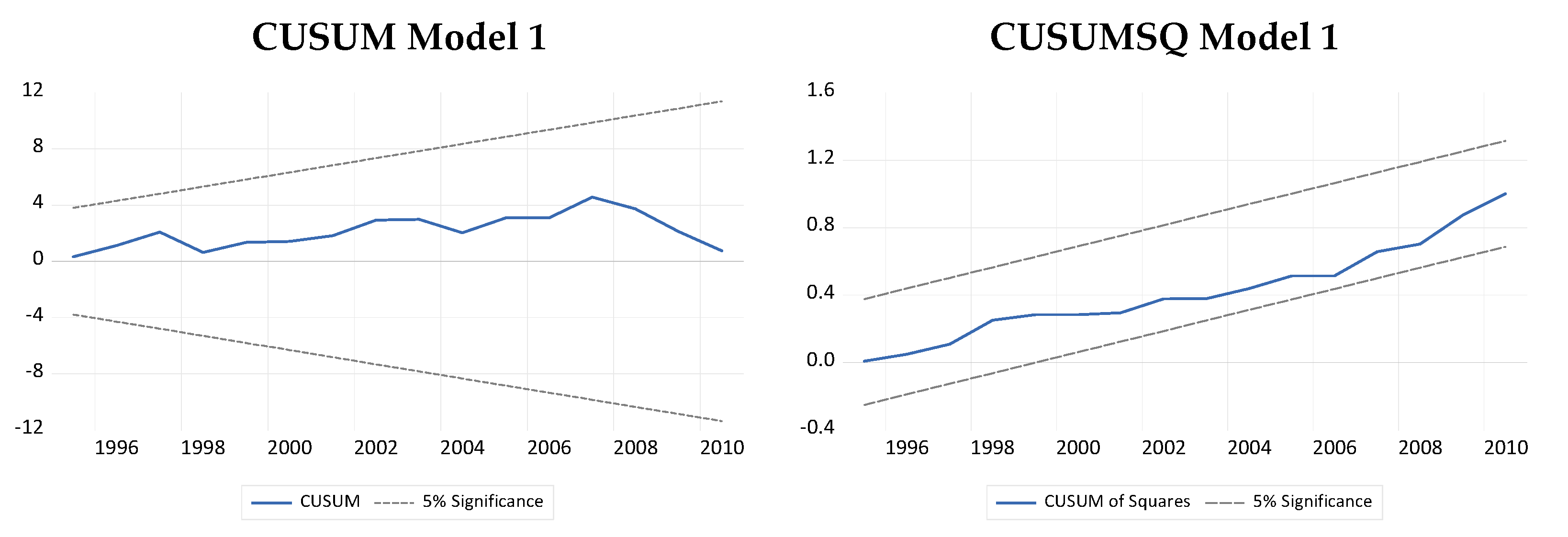
For analysis of the stability of the parameters over the sample period we (re)estimated both models using recursive least squares, and, additionally, we used the cumulative sum control chart (CUSUM) and the cumulative sum control chart of squares (CUSUMSQ) tests.
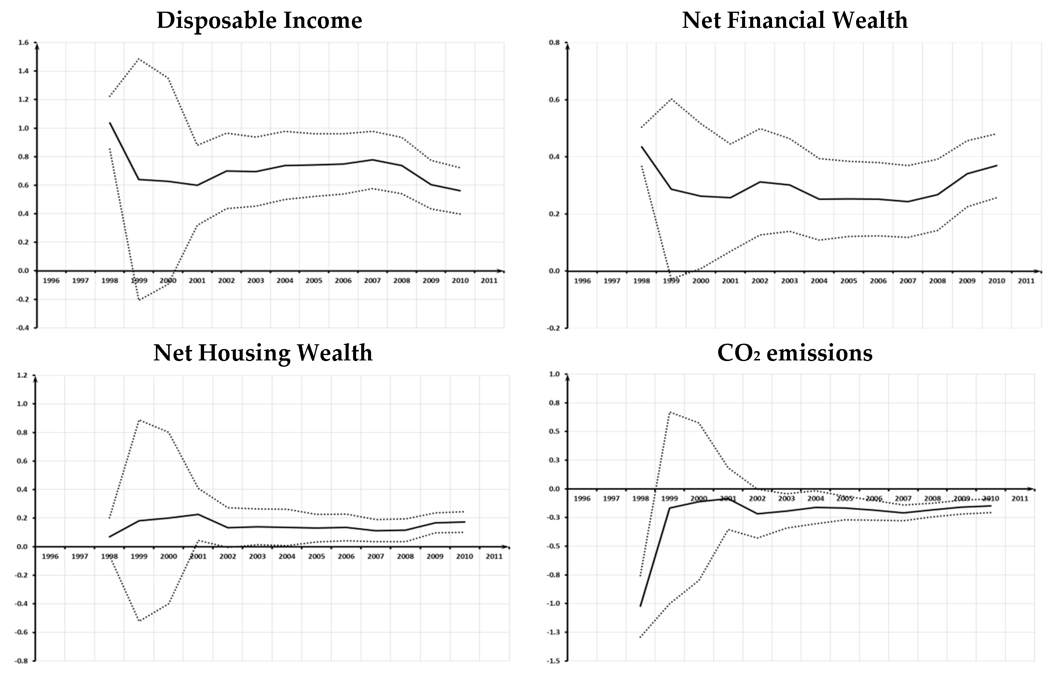
The recursive least squares procedure suggests that the time pattern of the estimated parameters was not affected by the structural changes in the composition of household wealth after 2000 for Model 1 (see Figure 4). However, in the disaggregated wealth model, the parameters of disposable income and financial wealth show slight variability during the sample period, while the estimated coefficients of housing wealth and CO2 emissions are much more stable. In addition, in the CUSUM and CUSUMSQ tests (see Figure 3), the accumulated sums never cross the bounds of the 5% confidence level, so the null hypothesis of the stability of the parameters is not rejected. We confidently conclude that the estimated coefficients are stable for both models over the sample period.

7. Summary and Conclusions

In this paper we present evidence of the effect of CO2 emissions from burning fossil fuels and cement production on aggregate nondurables household’s consumption in Portugal, using data from 1980 to 2014. Using a dynamic ordinary least squares procedure, we estimate a consumption function based on the life cycle and permanent income hypothesis extended to accommodate the effects of CO2 emissions. We consider two variants of this consumption function approach, one with aggregate wealth and the other considering separately financial and housing wealth.
In general terms, all of the estimated parameters are highly significant and consistent with the relevant conceptual requirements. In the aggregate wealth model, our results suggest that an increase of EUR 1.00 in disposable income will cause an increase in consumption of EUR 0.45, while the same wealth stimulus causes an increase in consumption of EUR 0.10. In the disaggregated wealth model, the results indicate that consumption is more sensitive to changes in financial wealth than housing wealth for the same causal disturbance.
Our results point overwhelmingly to the conclusion that CO2 emissions have a negative effect on the marginal utility of consumption. Accordingly, a reduction of CO2 emissions leads to increased consumption demand. Indeed, our findings suggest that there is a substitution relationship between CO2 emissions and household consumption expenditure, i.e., a distaste effect. Specifically, a reduction in emissions will cause an increase in consumption of EUR 0.14 when we consider aggregate wealth and EUR 0.17 when we consider disaggregated wealth. This result is also in line with negative state dependence, according to which improvements in health are complementary to the increase in consumption for good health. Accordingly, reducing pollution will improve health conditions, which affects permanent income and stimulates consumption for good health—for example, increasing one’s practice of regular physical exercise, healthy eating or leisure activities, particularly related to active aging.

8. Policy Implications

Our results, have several important policy implications. First and foremost, our results on the relationship between CO2 emissions and household consumption suggest that it is possible to reconcile the decarbonization of the economy with the increase in household consumption. This is a critical piece of information in determining the likelihood of adoption and the potential for success of such decarbonization policies.
Second, our findings on the relationship between CO2 emissions and household consumption have implications for the existence of endogenous limit cycles in consumption spending. These depend where the economy lies in the environmental Kuznets curve. Indeed, cyclical behavior of household consumption under the distaste effect arises only when the economy lies on the downward-sloping branch of the curve (see [10]). Forward-looking households perceive an exogenous decrease in pollution as both an improvement in their health conditions and as an increase in their permanent income. Under the distaste effect, households increase their consumption for good health while decreasing savings. If the economy is on the downward-sloping branch of the EKC, the fall in capital stock induced by the decrease in savings causes pollution to rise in the next period, giving rise to a deterministic cycle.
Furthermore, the existence of deterministic cycles also depends on savings behavior during the cycle. In particular, with intertemporal dependent preferences, saving may be determined by economic growth and not the way around, and thus be complementary to consumption (see [11]) In this context, forward-looking households will tend to smooth their consumption for the same reasons that households operating under the constant relative risk aversion smooth their consumption, regardless of distaste or compensation being the dominant effect. Indeed, under the distaste effect, reducing pollution will increase consumption as well as savings due to the presence of a habit-formation process in the utility function. In a richer, healthier and cleaner economy, the rise in capital stock induced by the increase in savings reduces pollution emissions in the next period so that the deterministic cycle subsides.
Our work suggests several avenues for future research. The first would be to identify the short- and long-term inertial properties of aggregate consumption expenditure. This is of crucial importance for understanding the smoothing process of household consumption and how that is affected by shocks in CO2 emissions. The second would to carry out further analysis on the effects of consumption on marginal utility using micro data on household consumption expenditures rather than aggregate consumption. This would allow for a finer identification of potentially different effects, both qualitatively and quantitatively for different income groups. Third, the success of environmental policies goes hand in hand with substantial changes in the composition of household consumption. Our study does not allow an assessment of whether or not the changes in both the pattern and the composition of the Portuguese household consumption are in line with the goals of responsible consumption (see [53]). In this context, an important extension of this work would be to focus on the issue of the composition of consumption not just on the effects on its level.
In a related vein, given that the branch of the environmental Kuznets curve on which the economy lies is a determining factor in cyclical behavior of consumption, the estimation of an environmental Kuznets curve using recent data for Portugal would be a natural extension of this paper. It should be noted that the existing literature of the Portuguese case only covers a time frame in which the economy is at the upward-slope part of the curve. Recent data, however, hints at the fact that from in the last two decades, the complementarity that had historically characterized the relationship between CO2 emissions and capital stock in the Portuguese economy may have been reversed. This suggests that, currently, the country is beyond the turning point of the curve and thus already lies on the downward-slope branch of the curve. This is of key relevance to determine the implications of the distaste effect identified in this paper.

Supplementary Materials

The following are available online at https://www.mdpi.com/article/10.3390/su132112153/s1.

Author Contributions

Conceptualization, J.M.B. and A.M.P.; Formal analysis, J.M.B.; Methodology, J.M.B. and A.M.P.; Writing—original draft, J.M.B.; Writing—review & editing, A.M.P. All authors have read and agreed to the published version of the manuscript.

Funding

This research received no external funding.

Institutional Review Board Statement

Not applicable.

Informed Consent Statement

Not applicable.

Data Availability Statement

Data sharing not applicable.

Acknowledgments

The first author would like to acknowledge financial support from FCT—Fundação para a Ciência e a Tecnologia (grant UID/ECO/04007/2020).

Conflicts of Interest

The authors declare no conflict of interest.

References

  1. Dasgupta, P.; Heal, G. The Optimal Depletion of Exhaustible Resources. Rev. Econ. Stud. 1974, 3, 28. [Google Scholar] [CrossRef]
  2. Tahvonen, O.; Kuuluvainen, J. Economic Growth, Pollution and Renewable Resources. J. Environ. Econ. Manag. 1993, 24, 101–118. [Google Scholar] [CrossRef]
  3. Eakin, D.; Selde, T. Stoking the fires? CO2 emissions and economic growth. J. Public Econ. 1995, 57, 85–101. [Google Scholar] [CrossRef] [Green Version]
  4. Michell, P.; Rotillon, G. Disutility of Pollution and Endogenous Growth. Environ. Resour. Econ. 1995, 6, 279–300. [Google Scholar]
  5. Smulders, S. Endogenous Growth Theory and the Environment. In Handbook of Environmental and Resource Economics; van der Berg, J.C.J.M., Ed.; Edward Elgar: Cheltenham, UK, 1999. [Google Scholar]
  6. Smulders, S. Economic Growth and Environmental Quality. In Principles of Environmental Economics; Folmer, H., Gabel, L., Eds.; Edward Elgar: Cheltenham, UK, 2000. [Google Scholar]
  7. Xepapadeas, A. Economic Growth and the Environment. In Handbook of Environmental Economics, 1st ed.; Mäler, K., Vincent, J., Eds.; Elsevier: Amsterdam, The Netherlands, 2005; Volume 3, pp. 1219–1271. [Google Scholar]
  8. Belbute, J.; Brito, P. On Sustainable Endogenous Growth Under Intertemporally Dependent Preferences. Icfai J. Environ. Econ. 2008, VI, 7–28. [Google Scholar]
  9. Kijima, M.; Nishide, K.; Ohyama, A. Economic models for the environmental Kuznets curve: A survey. J. Econ. Dyn. Control 2010, 34, 1187–1201. [Google Scholar] [CrossRef]
  10. Heal, G. The use of common property resources. In Explorations in Natural Resource Economics; Smith, V.K., Krutilla, J.V., Eds.; The Johns Hopkins University Press for Resources for the Future: Baltimore, MD, USA, 1982. [Google Scholar]
  11. Bosi, S.; Desmarchelier, D. Limit Cycles Under a Negative Effect of Pollution on Consumption Demand: The role of an environmental Kuznets Curve. Environ. Resour. Econ. 2018, 69, 343–363. [Google Scholar] [CrossRef] [Green Version]
  12. Carroll, C.D.; Overland, J.; Weil, D.N. Saving and Growth with Habit Formation. Am. Econ. Rev. 2000, 90, 341–355. [Google Scholar] [CrossRef]
  13. Finkelstein, A.; Luttmer, E.; Notowidigdo, M. What good is wealth without health? The effect of health on the marginal utility of consumption. J. Eur. Econ. Assoc. 2013, 11, 221–258. [Google Scholar] [CrossRef] [Green Version]
  14. WHO. World Health Organization Global Ambient Air Quality Database (Update 2018); WHO: Geneva, Switzerland, 2018. [Google Scholar]
  15. WHO. COP24 Special Report: Health and Climate Change; Licen/ce: CC BY-NC-SA 3.0 IGO; World Health Organization: Geneva, Switzerland, 2018. [Google Scholar]
  16. IPCC. Special Report on Global Warming of 1.5 °C (SR15); Intergovernmental Panel on Climate Change Annual Report, UNEP; UN: New York, NY, USA, 2018. [Google Scholar]
  17. Kampa, M.; Castanas, E. Human health effects of air pollution. Environ. Pollut. 2008, 151, 362–367. [Google Scholar] [CrossRef]
  18. Borowski, P.F. Environmental pollution as a threats to the ecology and development in Guinea Conakry. Environ. Prot. Nat. Resour. 2017, 28, 27–32. [Google Scholar] [CrossRef] [Green Version]
  19. Munksgaard, J.; Pedersen, K.; Wien, M. Impact of household consumption on CO2 emissions. Energy Econ. 2000, 22, 423–440. [Google Scholar] [CrossRef]
  20. Salo, M.; Nissinen, A. Consumption Choices to Decrease Personal Carbon Footprints of Finns; Report of the Finnish Environmental Institute, 30/2017; Finnish Environment Institute: Helsinki, Finland, 2017. [Google Scholar]
  21. QEPiC 2030. Quadro Estratégico da Política Climática; Agência Portuguesa do Ambiente: Lisboa, Portugal, 2015. [Google Scholar]
  22. RNC2050. Roteiro para a Neutralidade Carbónica/Roadmap for Carbon Neutrality; Agência Portuguesa do Ambiente: Lisboa, Portugal, 2019. [Google Scholar]
  23. UNFCC. The United Nations Framework Convention on Climate Change; COP24, COP25 and COP26; UN: New York, NY, USA, 1992. [Google Scholar]
  24. Żelaziński, T.; Ekielski, A.; Siwek, A.; Dardziński, L. Characterisation of corn extrudates with the addition of brewers’ spent grain as a raw material for the production of functional batters. Acta Sci. Polonorum. Technol. Aliment. 2017, 16, 247–254. [Google Scholar]
  25. Friedman, M. A Theory of the Consumption Function; Milton General Series No. 63; Princeton University Press: Princeton, NJ, USA, 1957. [Google Scholar]
  26. Ando, A.; Modigliani, F. The Life Cycle Hypothesis of Saving: Aggregate Implications and tests. Am. Econ. Rev. 1963, 53, 55–84. [Google Scholar]
  27. Hall, R.E. Stochastic Implications of the Life Cycle-Permanent Income Hypothesis: Theory and Evidence. J. Political Econ. 1978, 86, 971–987. [Google Scholar] [CrossRef]
  28. Phillips, P.; Durlauf, S. Multiple time series regression with integrated process. Rev. Econ. Stud. 1986, 53, 473–495. [Google Scholar] [CrossRef] [Green Version]
  29. Stock, J.; Watson, M. A Simple Estimator of Cointegrating Vectors in Higher Order Integrated Systems. Econometrica 1993, 61, 783–820. [Google Scholar] [CrossRef]
  30. Le Quére, C.; Moriarty, R.; Andrew, R.M.; Canadell, J.G.; Sitch, S.; Korsbakken, J.I.; Friedlingstein, P.; Peters, G.P.; Andres, R.J.; Boden, T.A.; et al. Global Carbon Budget 2015. Earth System Science Data 2015, 7, 349–396. [Google Scholar] [CrossRef] [Green Version]
  31. Boden, T.A.; Marland, G.; Andres, R.J. Global, Regional, and National Fossil-Fuel CO2 Emissions; Carbon Dioxide Information Analysis Center, Oak Ridge National Laboratory, U.S. Department of Energy: Oak Ridge, TN, USA, 2016. [CrossRef]
  32. Lettau, M.; Ludvigson, S. Understanding trend and cycle in asset values: Reevaluating the wealth effect on consumption. Am. Econ. Rev. 2004, 94, 276–299. [Google Scholar] [CrossRef] [Green Version]
  33. Castro, G. The wealth effect on consumption in the Portuguese economy. Econ. Bull. 2007, 13, 37–55. Available online: https://www.bportugal.pt/sites/default/files/anexos/papers/ab200713_e.pdf (accessed on 12 August 2021).
  34. Sousa, R. Wealth Effects on Consumption: Evidence from the Euro Area. Banks Bank Syst. 2010, 5, 70–78. [Google Scholar]
  35. Belbute, J.; Pereira, A. An Alternative Reference Scenario for Global CO2 Emissions from Fuel Consumption: An ARFIMA Approach. Econ. Lett. 2015, 135, 108–111. [Google Scholar] [CrossRef] [Green Version]
  36. Belbute, J.; Pereira, A. Do Global CO2 Emissions from Fossil-Fuel Consumption Exhibit Long Memory? A Fractional Integration Analysis. Appl. Econ. 2017, 49, 4055–4070. [Google Scholar] [CrossRef]
  37. Shin, Y. A Residual–based test of the null of cointegration against the alternative of no cointegration. Econom. Theory 1994, 10, 91–115. [Google Scholar] [CrossRef] [Green Version]
  38. Engle, R.; Granger, C. Cointegration and error correction representation: Estimation and testing. Econometrica 1987, 55, 251–276. [Google Scholar] [CrossRef]
  39. Newey, W.; West, K. A Simple, Positive Semi-definite, Heteroskedasticity and Autocorrelation Consistent Covariance Matrix. Econometrica. 1987, 55, 703–708. [Google Scholar] [CrossRef]
  40. Charemza, W. Cointegration in Small Samples: Empirical Percentiles, Drifting Moments and Customized Testing. Oxf. Bull. Econ. Stat. 1990, 52, 303–315. [Google Scholar]
  41. Mackinnon, J. Critical Values for Cointegration Tests. In Long Run Economic Relationships, Readings in Cointegration; Granger, C., Engle, R., Eds.; Oxford University Press: Oxford, UK, 1991. [Google Scholar]
  42. Johansen, S. Statistical Analysis of Cointegration Vectors. J. Econ. Dyn. Control 1988, 12, 231–254. [Google Scholar] [CrossRef]
  43. Osterwald-Lenum, M. A Note with Quantiles of the Asymptotic Distribution of the Maximum Likelihood Cointregration Rank Test Statistics. Oxf. Bull. Econ. Stat. 1992, 54, 461–472. [Google Scholar] [CrossRef]
  44. Cardoso, F.; Farinha, L.; Lameira, R. Household Wealth in Portugal, Revised Series; Occasional Papers, 1/2008; Bank of Portugal: Lisboa, Portugal, 2008. [Google Scholar]
  45. Poterba, J.; Samwick, A. Stock Ownership Patterns, Stock Market Fluctuations and Consumption. Brook. Pap. Econ. Act. 1995, 2, 295–372. [Google Scholar] [CrossRef] [Green Version]
  46. Case, K.; Shiller, R.; Quigley, J. Comparing Wealth Effects: The Stock Market Versus the Housing Market. Adv. Macroecon. 2005, 5, 1–32. [Google Scholar] [CrossRef]
  47. Jarque, C.; Bera, A. Efficient tests for normality, homoscedasticity and serial independence of regression residuals. Econ. Lett. 1980, 6, 255–259. [Google Scholar] [CrossRef]
  48. White, H. A Heteroskedasticity-Consistent Covariance Matrix Estimator and a Direct Test for Heteroskedasticity. Econometrica 1980, 48, 817–838. [Google Scholar] [CrossRef]
  49. Breusch, T.; Pagan, A. A Simple Test for Heteroskedasticity and Random Coefficient Variation. Econometrica 1979, 47, 1287–1294. [Google Scholar] [CrossRef]
  50. Engle, R.F. Autoregressive conditional heteroskedasticity with estimates of the variance of U.K. inflation. Econometrica 1982, 50, 987–1008. [Google Scholar] [CrossRef]
  51. Breusch, T. Testing for Autocorrelation in Dynamic Linear Models. Aust. Econ. Pap. 1978, 17, 334–355. [Google Scholar] [CrossRef]
  52. Godfrey, L. Testing Against General Autoregressive and Moving Average Error Models when the Regressors Include Lagged Dependent Variables. Econometrica 1978, 46, 1293–1301. [Google Scholar] [CrossRef]
  53. Agenda 2030. The EU Strategy on Adaptation to Climate Change, European Commission (2014). A Policy Framework for Climate and Energy in the Period 2020 up to 2030. Communication from the Commission. Available online: http://bit.ly/1Qs1ZKx (accessed on 17 March 2017).
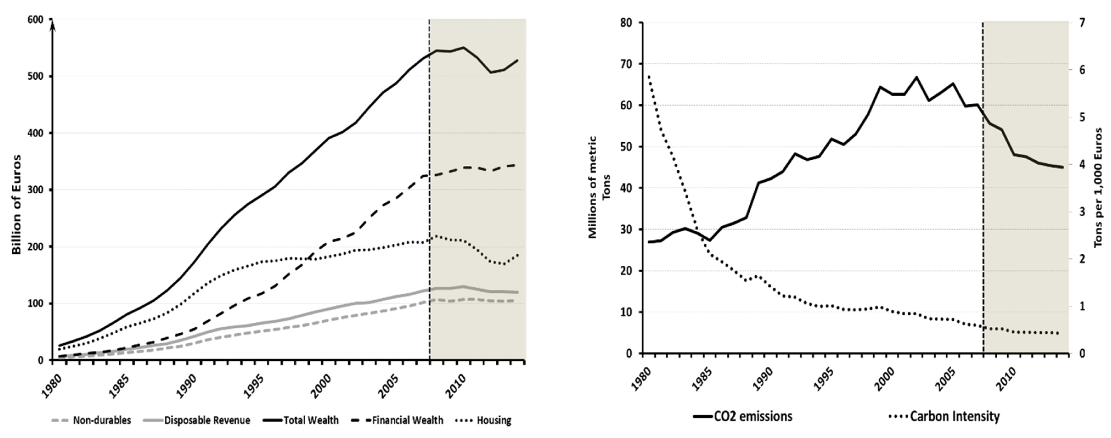
Figure 1. The Evolution of the Economic Variables and of CO2 Emissions.
Sustainability 13 12153 g001
Figure 2. Stability of the Estimated Coefficients using Recursive Least-Squares (RLS): Model 1.
Sustainability 13 12153 g002aSustainability 13 12153 g002b
Figure 3. Stability of the Estimated Coefficients using Recursive Least-Squares (RLS): Model 2.
Sustainability 13 12153 g003
Figure 4. Stability Analysis: CUSUM and CUSUMSQ tests.
Sustainability 13 12153 g004aSustainability 13 12153 g004b
Table 1. Economic Variables and CO2 Emissions: Basic Information.
Disposable IncomeNondurable ConsumptionTotal Net Wealth Shares (%)CO2 Emissions (106 Tons)Carbon Intensity 1
106 EurosNet Finantial WealthNonmortage Housing Wealth
1980–198512,254.038412.3049,943.9327.2972.7128.333.80
1986–199031,138.3821,998.52127,447.6731.0468.9635.671.66
1991–199557,969.1643,981.90251,332.2737.3962.6147.711.10
1996–200079,156.9861,760.26348,464.2548.4251.5857.680.93
2001–2005103,168.5082,926.64444,950.1455.9744.0363.790.77
2006–2010124,121.80103,042.34536,522.4860.5939.4155.540.54
2011–2014121,452.53105,214.23519,635.4765.2934.7145.990.44
Overall sample
μ72,488.8158,282.26312,051.1345.4954.5147.311.42
seμ7016.996073.3230,534.062.362.362.120.21
CV0.100.100.100.050.040.040.15
Notes: μ, seμ and CV stand for the mean, standard error and coefficient of variation respectively. 1 Tons of CO2 emissions per euro spend in nondurable consumption goods and services.
Table 2. ADF unit roots tests.
VariablesDeterministic ComponentLagst-Stat ADFBIC
Logs
Consumption of nondurablesConstant and trend0−3.041−147.153
Disposable incomeConstant and trend1−2.101−142.136
Net total wealthNone10.516−140.927
Net finantial wealthConstant and trend0−1.094−132.537
Non finantial wealth (housing)None10.652−108.157
Per capita CO2 emissionsConstant0−1.870−83.047
First Differences (Logs)
Consumption of nondurablesConstant and trend1−3.564**−137.999
Disposable incomeNone0−2.283**−141.462
Net total wealthNone0−2.507**−144.142
Net finantial wealthConstant and trend1−5.700***−128.928
Non finantial wealth (housing)None0−2.105**−111.204
Percapita CO2 emissionsConstant and trend0−6.124***−79.558
Notes: The critical values for a 1%, 5% and 10% significance ADF unit root test are: None: −2.62, −1.95, and −1.61; Constant: −3.58, −2.93, and −2.60; Constant and trend; −4.15, −3.50, and −3.18. In turn ** and *** stand for 0.01 < p < 0.05 and p < 0.01, respectively.
Table 3. Shin’s Cointegration Test.
LagsCμ
Model 1Model 2
10.0810.037
20.0860.050
30.1090.063
40.1410.087
Critical value (5%)0.159
Table 4. Augmented Engle-Granger Cointegration Tests.
Deterministic ComponentLagst-Stat ADFBIC
Model 1
None0−4.932***−164.356
Constant0−4.823**−161.137
Constant and trend3−4.930**−143.678
Model 2
None0−6.293***−168.912
Constant0−6.150***−165.875
Constant and trend0−6.145***−163.795
Note: We use [38] for “None” and [39] for “Constant” and “Constant and Trend” critical values. In this Table ** and *** stand for 0.01 < p < 0.05 and p < 0.01, respectively.
Table 5. Johansen’s Cointegration Tests.
Eigenvaluesλ-Trace Testλ-Max Test
H0HAStatisticCritical ValueH0HAStatisticCritical Value
Model 1 (Aggregate Wealth)
0.976r = 0r ≥ 1157.2853.12*r = 0r = 1127.0228.14*
0.414r ≤ 1r = 230.2634.91 r ≤ 1r = 218.1622.00
0.255r ≤ 2r = 312.1019.96 r ≤ 2r = 310.0315.67
0.059r ≤ 3r = 42.079.24 r ≤ 3r = 42.079.24
Model 2 (Disaggregate Wealth)
0.661r = 0r ≥ 192.6876.07*r = 0r = 135.6834.40*
0.531r ≤ 1r = 252.0053.12 r ≤ 1r = 224.9528.14
0.411r ≤ 2r = 332.0434.91 r ≤ 2r = 317.4622.00
0.251r ≤ 3r = 414.5919.96 r ≤ 3r = 49.5515.67
0.142r ≤ 4r = 55.049.24 r ≤ 4r = 55.049.24
Note: * stands for the rejection at the 95% critical values.
Table 6. Regression Results and Diagnostic Analysis.
ParameterModel 1Model 2
ElasticityMPCElasticityMPC
Contant (α)−2.457(0.215)*** −1.273(0.157)***
Disposable Income (βyd)0.588(0.076)***0.450.561(0.071)***0.43
Net Wealth (βw)0.575(0.077)***0.10
Net Financial Wealth (βwf) 0.369(0.054)***0.16
Net Housing Wealth (βwh) 0.174(0.018)***0.06
CO2 Emissions (βco2)−0.121(0.021)***−0.14−0.148(0.021)***−0.17
Diagnostic Analysis
Residual Sum of Squares (RSS)0.002 0.001
DW2.011 2.007
Log-Likelihood87.635 94.003
BIC−142.689 −146.652
RESET (F-test)3.906[0.067] 1.109[0.313]
F-Test (all coefficients)35,166[0.000] 176,189[0.000]
F[m,(T-k)] test for βco2 = 029.963[0.000] 27.111[0.000]
Jarque-Bera2.967[0.227] 0.360[0.835]
LM-White test20.720[0.294] 20.425[0.672]
LM-Breusch-Pagan test 4.402[0.883] 7.622[0.814]
LM-ARCH (1)1.386[0.239] 1.948[0.163]
LM-ARCH (5)2.149[0.828] 4.736[0.449]
LM-ARCH (10)8.534[0.577] 7.772[0.651]
LM (2)0.304[0.858] 2.404[0.301]
LM (5)9.154[0.103] 21.639[0.001]
LM (10)17.632[0.062] 24.721[0.006]
Q10.059[0.965] 0.029[0.864]
Q55.205[0.391] 12.037[0.034]
Q1212.649[0.395] 21.042[0.051]
Q211.592[0.207] 2.210[0.137]
Q252.719[0.743] 8.328[0.139]
Q2129.300[0.677] 12.081[0.439]
Notes: Standard errors in curved brackets and p-values in square brackets; m stands for the number of restrictions, T is the number of observations and k is the number of parameters estimated in the unrestricted regression; MPC stands for marginal propensity to consume; *** p < 0.01.
Publisher’s Note: MDPI stays neutral with regard to jurisdictional claims in published maps and institutional affiliations.