
Simulation-Assisted Design Process of a 22 kW Wireless Power Transfer System Using Three-Phase Coil Coupling for EVs


Abstract
:1. Introduction
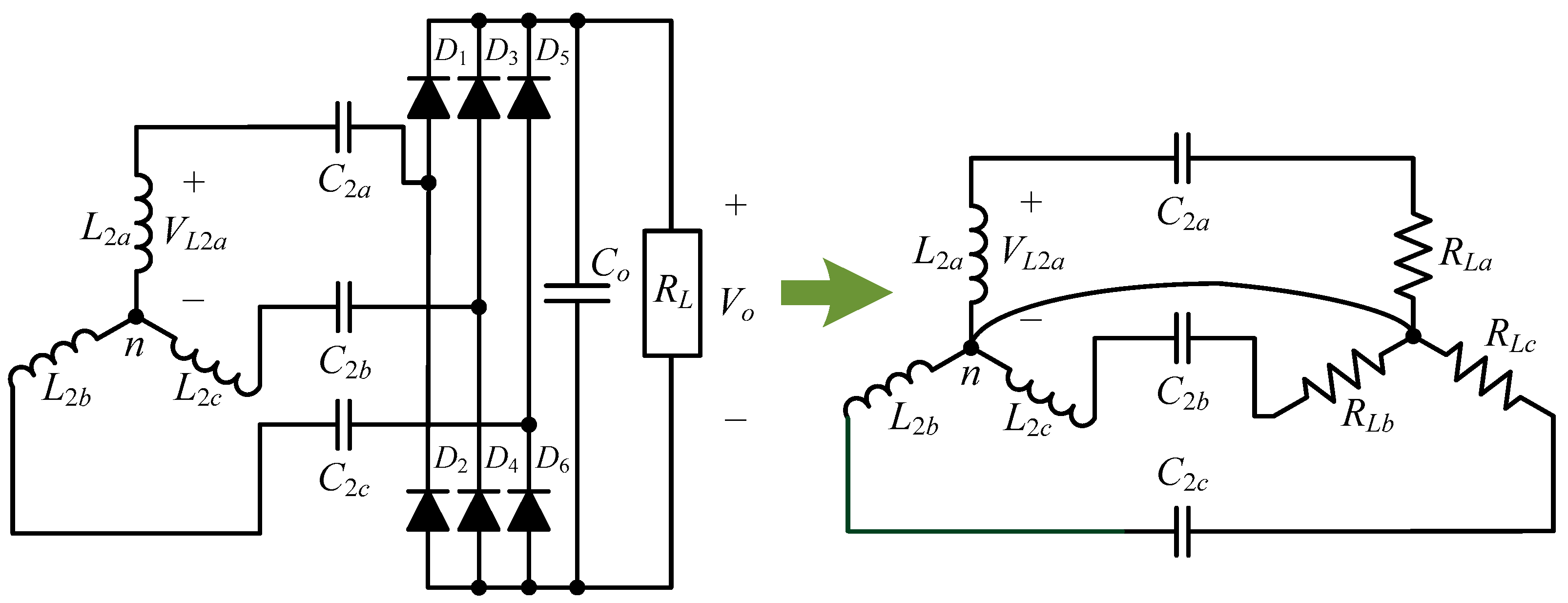
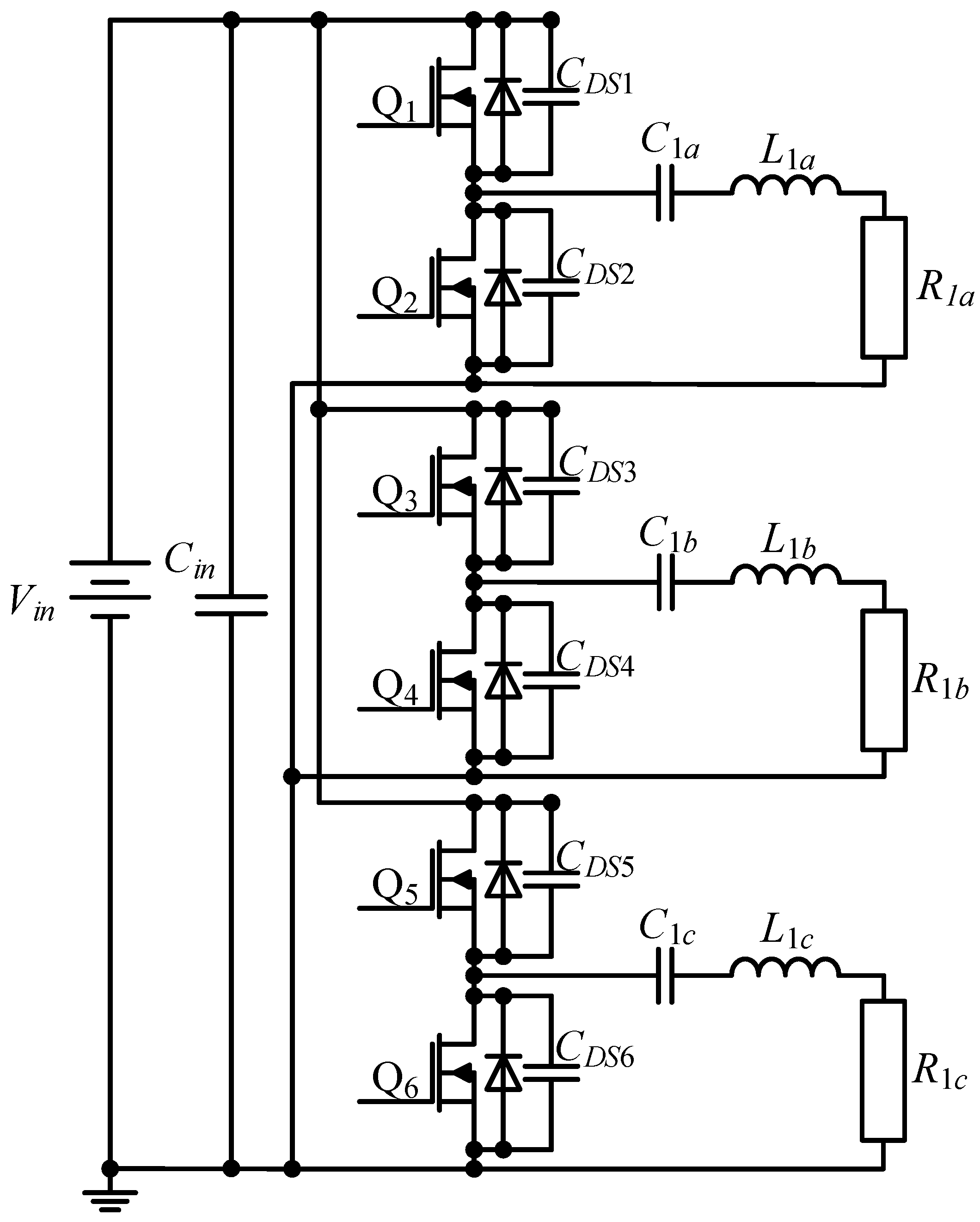
2. Circuit Topology
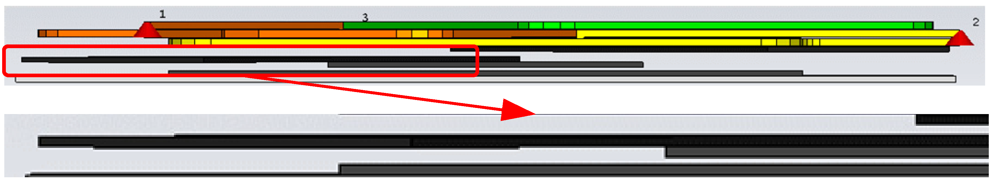
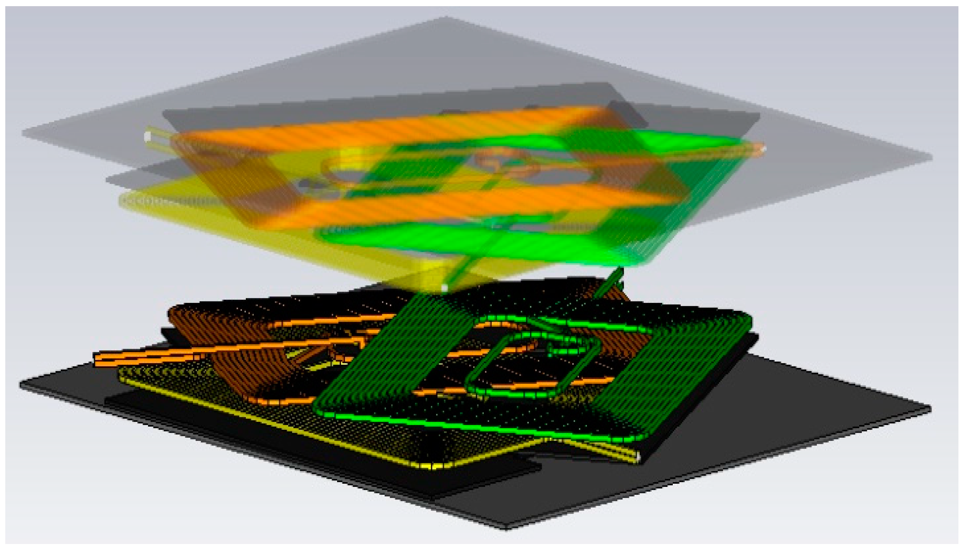
3. Coil Design
4. Results
5. Conclusions
Author Contributions
Funding
Institutional Review Board Statement
Informed Consent Statement
Data Availability Statement
Acknowledgments
Conflicts of Interest
References
- Michaelides, E.E. Primary Energy Use and Environmental Effects of Electric Vehicles. World Electr. Veh. J. 2021, 12, 138. [Google Scholar] [CrossRef]
- Garwa, N.; Niazi, K.R. Impact of EV on Integration with Grid System-A Review. In Proceedings of the International Conference on Power Systems, Perth, Australia, 10–12 October 2019; pp. 1–6. [Google Scholar]
- IEA. Global EV Outlook 2021, IEA, Paris. Available online: https://www.iea.org/reports/global-ev-outlook-2021 (accessed on 28 October 2021).
- Liu, D.; Zhang, T.; Wang, W.; Peng, X.; Liu, M.; Jia, H.; Su, S. Two-Stage Physical Economic Adjustable Capacity Evaluation Model of Electric Vehicles for Peak Shaving and Valley Filling Auxiliary Servicses. Sustainability 2021, 13, 8153. [Google Scholar] [CrossRef]
- Brenna, M.; Foiadelli, F.; Leone, C. Electric Vehicles Charging Technology Review and Optimal Size Estimation. J. Electr. Eng. Technol. 2020, 15, 2539–2552. [Google Scholar] [CrossRef]
- Lu, X.; Wang, P.; Niyato, D.; Kim, D.I.; Han, Z. Wireless charging technologies: Fundamentals, standards, and network applications. IEEE Commun. Surv. Tutor. 2016, 18, 1413–1452. [Google Scholar] [CrossRef] [Green Version]
- Bosshard, R.; Kolar, J.W. Inductive power transfer for electric vehicle charging: Technical challenges and tradeoffs. IEEE Power Electron. Mag. 2016, 3, 22–30. [Google Scholar] [CrossRef]
- Bojarski, M.; Asa, E.; Colak, K.; Czarkowski, D. A 25 kW industrial prototype wireless electric vehicle charger. In Proceedings of the IEEE Applied Power Electronics Conference Exposition, Long Beach, CA, USA, 20–24 March 2016; pp. 1756–1761. [Google Scholar]
- Mi, C.; Buja, G.; Choi, S.Y.; Rim, C.T. Modern Advances in Wireless Power Transfer Systems for Roadway Powered Electric Vehicles. IEEE Trans. Ind. Electron. 2016, 63, 6533–6545. [Google Scholar] [CrossRef]
- Matsumoto, H.; Shibako, Y.; Neba, Y. Contactless Power Transfer System for AGVs. IEEE Trans. Ind. Electron. 2018, 65, 251–260. [Google Scholar] [CrossRef]
- Joseph, P.K.; Elangovan, D.; Sanjeevikumar, P. System Architecture, Design, and Optimization of a Flexible Wireless Charger for Renewable Energy-Powered Electric Bicycles. IEEE Syst. J. 2020, 15, 2696–2707. [Google Scholar] [CrossRef]
- Feng, H.; Tavakoli, R.; Onar, O.C.; Pantic, Z. Advances in High-Power Wireless Charging Systems: Overview and Design Considerations. IEEE Trans. Transp. Electrif. 2020, 6, 886–919. [Google Scholar] [CrossRef]
- Pathmanathan, M.; Nie, S.; Yakop, N.; Lehn, P.W. Field-Oriented Control of a Three-Phase Wireless Power Transfer System Transmitter. IEEE Trans. Transp. Electrif. 2019, 5, 1015–1026. [Google Scholar] [CrossRef]
- Pries, J.; Galigekere, V.P.N.; Onar, O.C.; Su, G.-J. A 50-kW Three-Phase Wireless Power Transfer System Using Bipolar Windings and Series Resonant Networks for Rotating Magnetic Fields. IEEE Trans. Power Electron. 2019, 35, 4500–4517. [Google Scholar] [CrossRef]
- Wang, C.; Zhu, C.; Wei, G.; Feng, J.; Jiang, J.; Lu, R. Design of Compact Three-Phase Receiver for Meander-Type Dynamic Wireless Power Transfer System. IEEE Trans. Power Electron. 2020, 35, 6854–6866. [Google Scholar] [CrossRef]
- Mohammad, M.; Pries, J.L.; Onar, O.C.; Galigekere, V.P.; Su, G.-J.; Wilkins, J. Three-Phase LCC-LCC Compensated 50-kW Wireless Charging System with Non-Zero Interphase Coupling. In Proceedings of the 2021 IEEE Applied Power Electronics Conference and Exposition (APEC), Phoenix, AZ, USA, 14–17 June 2021; pp. 456–462. [Google Scholar] [CrossRef]
- SAE J2954. Wireless Power Transfer for Light-Duty PlugIn/Electric Vehicles and Alignment Methodology. Available online: https://www.sae.org/standards/content/j2954_202010/ (accessed on 30 October 2021).
- Mohamed, A.; Marim, A.A.; Mohammed, O. Magnetic Design Considerations of Bidirectional Inductive Wireless Power Transfer System for EV Applications. IEEE Trans. Magn. 2017, 53, 1–5. [Google Scholar] [CrossRef]
- Safaee, A.; Woronowicz, K.; Maknouninejad, A. Reactive Power Compensation Scheme for an Imbalanced Three-Phase Series-Compensated Wireless Power Transfer System with a Star-Connected Load. In Proceedings of the IEEE Transportation Electrification Conference 316 and Expo, Long Beach, CA, USA, 13–15 June 2018; pp. 44–48. [Google Scholar]


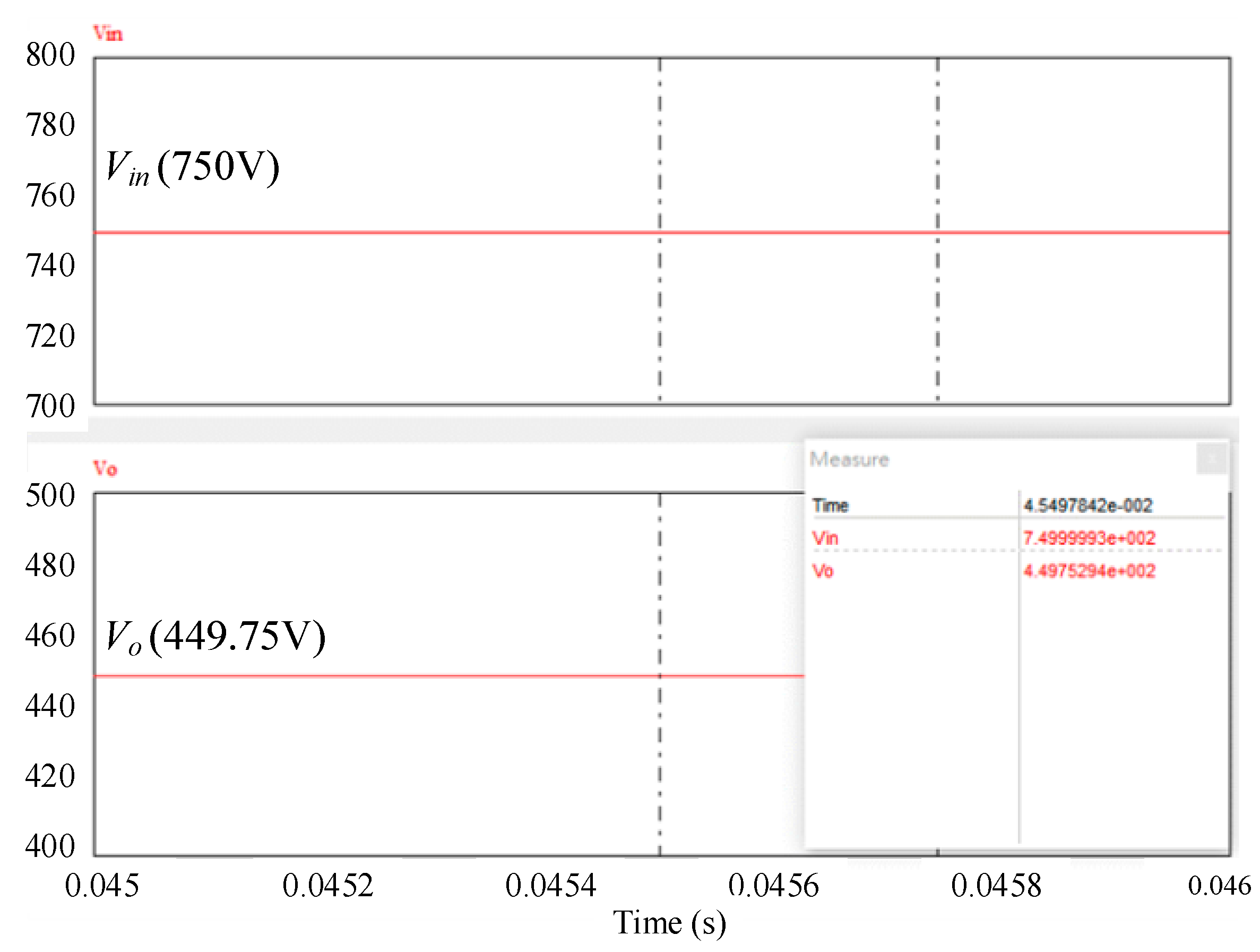
| Inverter input voltage (Vin) | 750 V |
| Rectifier output voltage (Vo) | 450 V |
| Output power (Po) | 22 kW |
| Operating frequency | 85 kHz |
| Transmission distance (air gap) | 170 mm~250 mm |
| Coil Type | Tx/Rx Coils |
| Size | 600 mm × 450 mm |
| Number of turns | 14 |
| Wire thickness | 8 mm |
| Magnetic material specification | |
| Magnetic material | Ferrite FAT100 xiaoshuang(Crown Ferrite Enterprise Co.) |
| Magnetic material size | 882 m × 763 mm |
| Magnetic material thickness | 5 mm |
| Magnetic field shielding plates | |
| Shielding plate material | Aluminum |
| Shielding plate size | 890 mm × 780 mm |
| Shielding plate thickness | 6 mm |
| Items | Tx Coils | Rx Coils | ||||
|---|---|---|---|---|---|---|
| Self-inductance (μH) | L1a | L1b | L1c | L2a | L2b | L2c |
| 131 | 131.1 | 130.3 | 130.9 | 130.6 | 130.7 | |
| Mutual inductance (μH) | M1b1a | M1c1b | M1a1c | M1b1a | M1c1b | M1a1c |
| 33.26 | 33.69 | 35.6 | 35.67 | 33.64 | 33.07 | |
| Primary coils (μH) | L1a | L1b | L1c | M1b1a | M1c1b | M1a1c |
| 131 | 131.1 | 130.3 | 33.26 | 33.69 | 35.6 | |
| Secondary coils (μH) | L2a | L2b | L2c | M2b2a | M2c2b | M2a2c |
| 130.9 | 130.6 | 130.7 | 35.67 | 33.64 | 33.07 | |
| Output resistor RL | Simulation (9.2 Ω) | Calculation (9 Ω) | ||||
| Mutual inductance (μH) | M1a2a | M1b2a | M1c2a | |||
| 29.96 | 13.13 | 12.02 | ||||
| Primary side capacitors (nF) | Simulation | Calculation | ||||
| C1a | C1b | C1c | C1a | C1b | C1c | |
| 36.6 | 35.2 | 37.2 | 39 | 34.5 | 36.5 | |
| Secondary side capacitors (nF) | Simulation | Calculation | ||||
| C1a | C1b | C1c | C1a | C1b | C1c | |
| 36.6 | 37.2 | 35.2 | 37 | 37 | 35 | |
| Primary coils | L1a | 161.79 μH | Secondary coils | L2a | 158.69 μH | |
| L1b | 152.86 μH | L2b | 160.25 μH | |||
| L1c | 158.83 μH | L2c | 164.07 μH | |||
| M1b1a | 35.56 μH | M2b2a | 41.20 μH | |||
| M1c1b | 39.52 μH | M2c2b | 41.25 μH | |||
| M1a1c | 37.30 μH | M2a2c | 37.82 μH | |||
| Mutual inductances | M1a2a | 36.40 μH | M1b2a | 16.89 μH | M1c2a | 14.76 μH |
| M1a2b | 13.84 μH | M1b2b | 36.56 μH | M1c2b | 14.81 μH | |
| M1a2c | 14.81 μH | M1b2c | 16.81 μH | M1c2c | 37.84 μH | |
Publisher’s Note: MDPI stays neutral with regard to jurisdictional claims in published maps and institutional affiliations. |
© 2021 by the authors. Licensee MDPI, Basel, Switzerland. This article is an open access article distributed under the terms and conditions of the Creative Commons Attribution (CC BY) license (https://creativecommons.org/licenses/by/4.0/).
Share and Cite
Wu, C.-H.; Lai, C.-M.; Mishima, T.; Liang, Z.-B. Simulation-Assisted Design Process of a 22 kW Wireless Power Transfer System Using Three-Phase Coil Coupling for EVs. Sustainability 2021, 13, 12257. https://doi.org/10.3390/su132112257
Wu C-H, Lai C-M, Mishima T, Liang Z-B. Simulation-Assisted Design Process of a 22 kW Wireless Power Transfer System Using Three-Phase Coil Coupling for EVs. Sustainability. 2021; 13(21):12257. https://doi.org/10.3390/su132112257
Chicago/Turabian StyleWu, Chia-Hsuan, Ching-Ming Lai, Tomokazu Mishima, and Zheng-Bo Liang. 2021. "Simulation-Assisted Design Process of a 22 kW Wireless Power Transfer System Using Three-Phase Coil Coupling for EVs" Sustainability 13, no. 21: 12257. https://doi.org/10.3390/su132112257
APA StyleWu, C.-H., Lai, C.-M., Mishima, T., & Liang, Z.-B. (2021). Simulation-Assisted Design Process of a 22 kW Wireless Power Transfer System Using Three-Phase Coil Coupling for EVs. Sustainability, 13(21), 12257. https://doi.org/10.3390/su132112257