Early Warning System for Online STEM Learning—A Slimmer Approach Using Recurrent Neural Networks

Abstract

While the use of deep neural networks is popular for predicting students’ learning outcomes, convolutional neural network (CNN)-based methods are used more often. Such methods require numerous features, training data, or multiple models to achieve week-by-week predictions. However, many current learning management systems (LMSs) operated by colleges cannot provide adequate information. To make the system more feasible, this article proposes a recurrent neural network (RNN)-based framework to identify at-risk students who might fail the course using only a few common learning features. RNN-based methods can be more effective than CNN-based methods in identifying at-risk students due to their ability to memorize time-series features. The data used in this study were collected from an online course that teaches artificial intelligence (AI) at a university in northern Taiwan. Common features, such as the number of logins, number of posts and number of homework assignments submitted, are considered to train the model. This study compares the prediction results of the RNN model with the following conventional machine learning models: logistic regression, support vector machines, decision trees and random forests. This work also compares the performance of the RNN model with two neural network-based models: the multi-layer perceptron (MLP) and a CNN-based model. The experimental results demonstrate that the RNN model used in this study is better than conventional machine learning models and the MLP in terms of F-score, while achieving similar performance to the CNN-based model with fewer parameters. Our study shows that the designed RNN model can identify at-risk students once one-third of the semester has passed. Some future directions are also discussed.

1. Introduction

The impact of COVID-19 has led to discussions in the field of information and communications technology (ICT) about the need for more schools to provide online programs, allowing students to learn in flexible and diversified ways. In addition to existing massive open online courses (MOOCs), many online platforms have begun to appear on the market. In these contexts, instructors may have limited information that can be helpful in detecting student attrition due to the lack of face-to-face interactions [1]. As a result, distance education has traditionally been associated with high drop-out rates, low completion rates and low success rates [2,3]. At the same time, one of the advantages of online learning platforms is that learning analytics can produce a large amount of behavioral information. In many ways, digital data may provide more useful and higher quality information compared to data collected through other, more traditional methods [4]. Such data from learning analytics could be used to help researchers provide suggestions for improving the learning experience. If the time students spend on the platform is extended, students’ learning outcomes could be improved; thus, the feasibility of the online open-course business model may be promoted [1]. Therefore, schools and universities have developed private learning platforms (i.e., learning management systems, LMS) which log students’ learning behaviors and instructors have attempted to utilize these data to improve the overall learning efficacy and to strengthen the students’ adherence to the courses both in online and offline settings [2,3,4].

For hybrid learning settings (e.g., a mix of online and face-to-face components), Lu et al. [5] developed a model that analyzed students’ online and offline behavior and predicted at-risk students one third of the way into the semester. Based on the analysis of the learning data, the use of the early warning system (EWS) served to predict students who were less likely to succeed before the end of the term. While the “hybrid” EWS could successfully alert students who were at risk of completing a course, at some level, the system still required “manual input” by the instructors in identifying vulnerable students.

However, in a fully online learning setting, the lack of asynchronous communication and interactions between the instructor and students can make it difficult for instructors to discern student success. The use of a system such as the EWS in making accurate predictions can be helpful in identifying problems among students early on. Current research suggests that EWS can be effective in both hybrid and fully online learning settings. The system serves to identify at-risk students and intervene in the early stages of the learning processes so that students have a better chance of completing the course [6].

In recent years, researchers have utilized artificial intelligence (AI) techniques, especially machine learning methods, for automated at-risk student predictions through the EWS [7]. Machine learning techniques have been used to predict students’ performance; however, most approaches do not consider the temporal relations that exist during learning [8]. Hence, this study determines whether we can have better prediction accuracy when temporal information is factored in the learning. Then, the aim of this study is to maintain the accuracy of other studies using deep neural networks (i.e., deep learning) to predict whether students would pass the course and to determine how early the prediction can be made while maintaining sufficient accuracy. Teachers can utilize this EWS in their online courses to more easily detect at-risk students. We believe that the EWS will not only assist teachers but will also help students maintain their learning performance.

The contribution of this article is summarized as follows:

• We developed an assessment of at-risk students based on their online learning behavior and provided information to teachers for devising early intervention strategies to improve students’ concentration in online courses.
• We provide a single, lightweight model that can make weekly predictions by leveraging the characteristics of RNN models, thus contributing to online learning platforms that deploy EWS.
• We conducted an experiment to show the effectiveness of the RNN model and we compare the employed RNN models to other machine learning and deep learning models. The employed RNN models demonstrated satisfactory results when there were few learning features.

The remainder of this article is organized as follows: Section 2 presents a broad review of recent works on EWS, especially the studies that applied machine learning technology. We also discuss their disadvantages. Section 3 introduces the methodology, feature descriptions and model settings applied in this study, followed by details of the experiments and discussions in Section 4 and Section 5, respectively.

2. Literature Review

As one of the mainstreams in the field of educational technology, learning analytics has become an influential method for sustaining students’ online learning [9]. The lives of the younger generation are filled with information in their daily digital media digest menu (e.g., social media, podcasting) and their real lives (e.g., jobs, student clubs, school activities), thus highlighting the need for and value of continuously keeping students on track through timely learning analytics reports, such as an EWS [10]. The results of an EWS are formative and can greatly help instructors warn students before they start to fail. Thus, the value of EWS as one type of learning analytics for the current era when nearly all courses occur online is strong. Learning analytics is defined as “an educational application of web analytics aimed at learner profiling, a process of gathering and analyzing details of individual student interactions in online learning activities” [11]. Many institutions have invested in and customized systems for specific needs. However, the option for investment has not been economic [12]. EWSs are normally built within the learning management system (LMS), where entire courses can be stored and administered online and are supported by various specific instructional needs.

In terms of developing EWS, many studies have applied conventional machine learning models. Bozkurt et al. [13] developed an extensive survey and summarized the research directions for using AI in education into several categories. One of these directions is applying deep learning and machine learning algorithms to online learning processes. Traditional machine learning focuses on the results of algorithms, with more emphasis on mathematical inferences that can be verified or results that can be interpreted by humans. Such learning usually generates rules based on data and has a wide range of applications in different fields, such as computer-assisted teaching [14], score prediction [15], decision systems [16], educational data mining [17,18,19] and teaching strategies [20]. Moreno-Marcos et al. [7] used machine learning models, including random forests (RFs), generalized linear models, support vector machines (SVMs) and decision trees (DTs), to predict which students were at risk. To attain a high accuracy level, selecting discriminative features and providing sufficient learning data are required. However, the selection of features among different courses varies and the prediction accuracy drops to 0.5–0.7 when only partial learning data are used.

Alternatively, many researchers [21,22,23] have used the multi-layer perceptron (MLP) model for automated risk prediction. Zeineddine et al. [21] compared the performance between the MLP model and conventional machine learning approaches, such as k-means, k-nearest neighbors, naive Bayes, SVMs, DTs and logistic regression (LR). The authors used 13 features in their study, most of which elaborated on the learners’ knowledge level but not their learning behaviors [21]. The accuracy of their results fell from 56% to 83%. The method proposed by Mutanu et al. [22] reached about 83% accuracy using parameters such as grade point average (GPA) before enrollment. Lee et al. [23] used the online learning behaviors of students before different exams to predict their scores on those exams. The accuracy was about 0.73–0.97 under different model settings.

In recent years, the ability of neural networks has greatly improved due to the development of deep learning techniques. Since deep learning has had many achievements in various fields, such as image recognition and natural language processing [24], some studies have started to adopt deep learning techniques in the educational field. For example, Du et al. [25] proposed a CNN-based model called Channel Learning Image Recognition (CLIR) and provided visualized results to let teachers observe the difference between the at-risk students and other students. In their study, they arranged the learning features each week as a two-dimensional image and applied CNN to make predictions [25]. With the data of 5235 students and 576 absolute features, the recall rate of the CLIR models they proposed was over 77.26%.

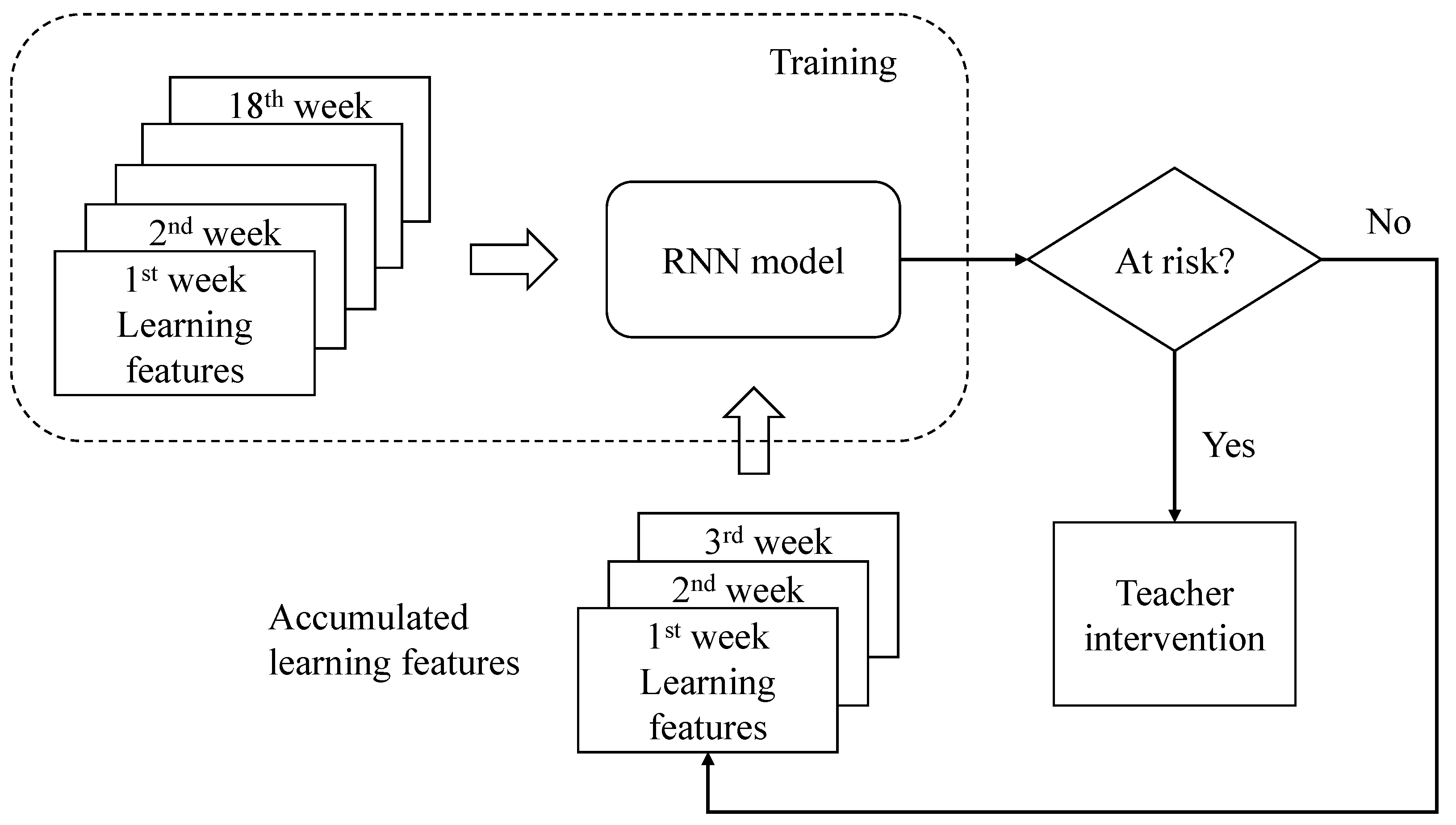
When facing incomplete learning data, a common practice is to fill zeros in those missing fields. However, if the provided learning data are accumulated during different learning periods, the performance of the model is drastically reduced even with such operations. To avoid filling in zeros, which may alter the distribution of data, previous studies [21,22,25,26] used the same length of time as the input when training the model. For example, if we want to predict the outcomes of students in the ninth week, we only provide the model with the cumulative nine weeks of data. However, in our opinion, it is not fair to decide whether a student passes or fails based on partial information. If the model is to be used in a real EWS, it should capture students’ learning patterns in that course across the entire semester and make accurate predictions before the end of the semester to identify and help students while they are still learning. Thus, the model used in this study was trained by providing the complete learning data for the entire semester and tested by only providing learning data over several weeks. By doing so, the model can learn the characteristics of students’ learning behavior throughout the course and make acceptable predictions with partial data.

When applying conventional machine learning, feature engineering (i.e., the selection of effective parameters to be included in the model) may be required to extract important features, while neural networks are much more convenient because they can extract useful features from raw data during the training process. Most studies have used MLP or CNN models for automated at-risk prediction. As the nature of these models tends to ignore the temporal information of raw data, this study chose another classic model: the recurrent neural network (RNN). Thus, this study used RNN in the EWS of online learning courses. RNN was first proposed by Hopfield [27] and has had tremendous achievements in natural language processing in recent years, benefiting from improvements in computer hardware [24,28]. RNN, the neural network we chose, has the characteristic of remembering time sequence variations. Many studies have proven that the RNN model performs better than the CNN model when analyzing sequential data and there have been discussions about applying RNN models to educational data [26,29]. However, these methods still require learning features that may not be provided by existing platforms.

Learning is the accumulation of knowledge. The absorption of previous knowledge impacts the following learning outcomes. However, most conventional machine learning models cannot afford this requirement. Although we can make the model learn from sequential data, these models do not naturally memorize the changes on the timeline. In our opinion, RNNs have the potential to learn students’ learning patterns over time and it is not possible to determine whether students would pass the semester in the first several weeks. Therefore, the model should provide a certain level of confidence of prediction (i.e., probability of failure as the aforementioned) for both the instructors and the students. To achieve this, we trained the network with complete learning data to make it memorize the characteristics of learning behavior at different stages and predict whether students would be at risk at some point in the future. Furthermore, the CLIR experiments were conducted based on numerous subjects and many learning logs. However, for a traditional online platform, it is difficult to collect such a large number of subjects and data. This study found a useful yet effective model that can capture learning patterns in a relatively smaller dataset with fewer learning features. This study also discusses the performance of CLIR on the collected dataset and compares it with RNN models.

In summary, although many researchers have incorporated machine learning or deep learning techniques with the EWS, these methods have some inconveniences. First, some models require many learning samples and features. Second, to make predictions every week, they have to train the individual model each week. This study aims to propose a simple framework that can be more widely applied to most online earning platforms. To achieve this, we use RNNs to explore the following three questions:

• Can RNN correctly predict the learning effectiveness of online course students?
• Can RNN discover at-risk students with incomplete learning data?
• With incomplete learning data, does RNN perform better than other conventional NN and machine learning approaches in terms of predicting at-risk students?

3. Methodology

3.1. Research Flow

Figure 1 shows the flow of this research. First, we collected student learning behavior data on an online course week by week. At the end of the semester, we eliminated students’ data that showed no learning activities in the semester. The remaining data were used to train the RNN model, which was then used to predict the probability of failure in the class each week. Positive predictions indicate that the teacher needs to intervene in the students’ learning conditions.

3.2. Network Architecture

The RNN architecture has many forms, depending on the application. Figure 2a shows the general network topology of an RNN. Essentially, an RNN takes the output of itself at the last timestamp as part of the input for the current timestamp, which is why the RNN is considered to have “memory.” Based on this architecture, the topology in Figure 2a can be “unfolded” over time to demonstrate the change in network states. An RNN can be divided into four types for prediction according to the relationship of input and output forms: one-to-one, one-to-many, many-to-one and many-to-many. Figure 2b shows a many-to-one type, which is often used for predicting a single result, such as sentiment analysis. Figure 2c shows a many-to-many type, which is typically used for language translation or video classification.

In a nutshell, an RNN model takes the input x_t at timestamp t and the hidden states h_t−1 at time t − 1 t006F compute the hidden state h_t and output y_t at time t using the following equations:

$$h_t={\sigma }_h\left(W_h{x}_t+U_h{h}_{t-1}+b_h\right)$$

(1)

$$y_t={\sigma }_y\left(W_y{h}_t+b_y\right)$$

(2)

where W_h, W_y, U_h, b_h and b_y are parameter matrices that can be trained; ${\sigma }_h$ and ${\sigma }_y$ are activation functions. In this study, ${\sigma }_h$ is the hyperbolic tangent (tanh) function and ${\sigma }_y$ is the logistic function, so the output y_t ranges from 0 to 1, which reflects the probability of whether a student would fail this course.

The EWS should be able to provide predictions only when given partial learning data (e.g., six weeks of learning history). As mentioned in Section 2, when developing the EWS, most previous approaches adopted students’ partial learning data and used students’ final scores as the learning target to train the model. However, this method is unsuitable because the partial data used to train the model may not reflect the true learning pattern for the entire semester. Hence, in our view, the model should be trained by the entire dataset and provide a reliable prediction based on partial data. To achieve this goal, this study adopts the many-to-many structure. The model is 18 units long, corresponding to the 18-week class. The test data were less than or equal to 18 weeks to test the performance of the model.

In addition, the course design of the data sources in this study used self-regulated learning and students were not required to take the midterm and final exams in weeks 9 and 18, respectively. Thus, students could have completed the final exam in week 15 and subsequent learning data would not have affected their results for this course. Since we only adopted their data up to the final exam, this would result in inconsistent learning data lengths if students finished their final exam before the 18th week. However, this situation would not affect the learning of RNN model.

This research study tested three popular RNN network structures: simple recurrent network (SRN), which is also known as the Elman Network [30]; long short-term memory (LSTM) [30]; and gated recurrent unit (GRU) [31]. The major difference among these structures is the internal design of hidden units. The input and output formats remain the same. More specifically, the input sequence for training in this study is 18, which corresponds to the students’ learning activities per week. To predict whether students would pass this course, this study used binary cross entropy as the loss function:

$$loss=\frac{1}{n}{{\displaystyle \sum }}_{i=1}^n-\left[y_i\log {\widehat{y}}_i+\left(1-y_i\right)\log \left(1-{\widehat{y}}_i\right)\right]$$

(3)

where y_i is the ground-truth label of the training sample, ${\widehat{y}}_i$ is the prediction result and n is the total number of training samples.

3.3. Feature Format

While many previous studies of online platforms have examined numerous learning features to train the model, many existing online platforms do not have such rich information. Hence, this study collected only five features that are often provided by many online platforms: number of video views, number of posts, the time of taking the midterm or final exam and the number of accomplished homework assignments.

Table 1. Feature Description.

Features	Description
Number of views on videos	The number of times that the video is watched in that week. Only videos that are watched for more than five minutes are considered valid.
Number of posts	The number of posts on the designated forum in that week. The number of posts is included in the calculation of the final score, but there is no standard.
Has taken midterm	A binary value that indicates whether the student has taken the mid-term exam.
Has taken final exam	A binary value that indicates whether the student has taken the final exam.
Number of finished homework assignments	How much homework out of six assignments did the student accomplish?
Passed (prediction target)	A binary value that indicates whether the student has passed the course that week.

describes the value of each feature. Non-binary features are normalized from zero to one.

4. Experiments and Discussions

4.1. Data Acquisition and Model Configuration

The data for this study were obtained from a general education course at a university in northern Taiwan. This course is a science course called “Introduction to Artificial Intelligence” and the learners are from all departments in that university. This course is fully online, meaning that all class assignments and exams are taken online. The students can view system announcements, homework and exams, while the teachers of this course can correct homework, set exams, issue announcements and check the learning status of students from their learning logs. The characteristic of this course is that learning progress is completely determined by the students. They can apply for and take the online exam at any time after satisfying certain class requirements. If students do not take exams until the 17th week, they are required to take the test in the last week. The learning data of 234 students from three classes were collected for the experiments. The dataset consisted of 126 males and 108 females. Among those, 34% of male students failed this class compared to 17% of females. Overall, fifty-five students (23%) failed this course, indicating that the distribution of the data is somewhat unbalanced. Figure 3 shows the mean and standard deviation for all students in each dimension at the 3rd, 6th, 9th and 18th week. In general, students who passed this course have higher values than those who failed in all dimensions. However, from Figure 3a, we can see that the value of every feature at the 3rd week is quite small and the standard deviation is very large at the first half of the semester in Figure 3a–c, showing that making predictions at the early stage of the semester from this dataset is challenging.

Because there were only 234 samples in this study, this study used five-fold cross validation to evaluate the performance of all models. That is, 80% of the data (187 students) was used for training and the remaining 20% (47 students) was used for testing. We computed precision, recall, $F_{\beta }$, TPR and FPR to evaluate the model. The definitions of these metrics are shown as follows:

$$Precision=\frac{tp}{tp+fp}$$

(4)

$$Recall=\frac{tp}{tp+fn}$$

(5)

$$F_{\beta }=\frac{\left(1+{\beta }^2\right)\times precision\times recall}{{\beta }^2\times precision+recall}$$

(6)

$$TPR=\frac{tp}{tp+fn}$$

(7)

$$FPR=\frac{fp}{fp+tn}$$

(8)

where tp stands for true positives, tn represents true negatives, fp is false positives, fn is false negatives and β is a user-defined factor. In the following experiments, β was set to 1 to consider precision and recall fairly. TPR stands for true positive rate, which refers to the exact Recall. FPR stands for false positive rate, which represents the proportion of negative samples that are detected as positive.

The numbers of hidden units in the SRN, LSTM and GRU models were all set to 18. All models were trained by 150 epochs and the optimizer was Adam [32]. The proposed method was implemented using Python and the Keras framework [33]. Figure 4 depicts the network structure of the LSTM, CNN and MLP used in this study.

Table 2. Number of parameters for different models.

	1-CLIR	3-CLIR	SRN	LSTM	GRU	CNN	MLP
Number of parameters	67,569	67,857	1111	4351	3361	3955	3961

shows the number of parameters of these networks. It is noticeable that the network structure of MLP and CNN were designed to have a number of parameters close to that of the RNN models.

4.2. Results

This subsection presents the findings of several analyses to respond to the research questions raised in this study.

4.2.1. Research Question 1: Can RNN Correctly Predict the Learning Effectiveness of Online Course Students?

Table 3. The averaged performance of RNN models when applying complete data.

	Accuracy	Precision	Recall	Fβ (β = 1)
SRN	0.93	0.87	0.88	0.87
LSTM	0.91	0.76	0.95	0.84
GRU	0.92	0.87	0.81	0.84
MLP	0.91	0.72	0.89	0.80
CNN	0.93	0.79	0.89	0.84

presents the prediction performance of the three RNN models using the complete 18 weeks of data. The threshold for the output ${\widehat{y}}_t$ was set to 0.65. All three models had high accuracy. While the LSTM model had a lower precision rate of 0.76, it had the best recall rate among the three models. Thus, it is not fair to say that the LSTM is worse than the other two models because it depends on the system’s strategy. On the students’ side, we may want a high precision rate, because many low-risk students would be notified. However, from the teachers’ viewpoint, we seek a high recall rate because we want to discover as many at-risk students as possible. The F-scores of the three models were all above 0.82, proving that the RNN model can be used to predict the learning outcomes of students. We included the other two popular models, MLP and CNN, in Table 3 for comparison.

Figure 5 depicts the receiver operating characteristic (ROC) curve of the three RNN models. We can see that the areas under the curve (AUCs) are quite close to each other. However, because the educational data are imbalanced, the ROC curve is affected by the negative samples (i.e., students who passed this course), which form the majority of the dataset. Hence, we conducted another experiment based on the average precision, the results of which are shown in Figure 6. The average precision of SRN, LSTM and GRU were 0.65, 0.77 and 0.68, respectively. From Figure 6, we observe that the LSTM model performed slightly better than the other two RNN models in terms of average precision, showing that the LSTM model performed best among three models in capturing the learning patterns of students who might fail this course.

Unlike the studies that use prediction accuracy to evaluate the performance of the model, this study considers the recall rate because educational data tend to be unbalanced, which may affect the accuracy. If students who perform well in class are predicted to be at-risk, there would be no harm. However, if truly at-risk students are missed by the model, we may lose the opportunity to help them, which would defeat the purpose of the EWS.

4.2.2. Research Question 2: Can RNN Discover At-Risk Students with Incomplete Learning Data?

In the first experiment, we verified that the RNN model could be used to estimate students’ learning outcomes. However, the EWS should not rely on the complete data to make predictions. Hence, in this experiment, we demonstrated the performance of RNN models when facing incomplete learning data.

First, the model was trained using the complete 18 weeks of learning data, as in the previous experiment. Then, we tested the trained model with incomplete learning data, ranging from 3 to 15 weeks.

Table 4. The F-score of the RNN models at different weeks.

	3rd Week	6th Week	9th Week	12th Week	15th Week	18th Week
SRN	0.44	0.51	0.56	0.55	0.63	0.87
LSTM	0.46	0.49	0.53	0.53	0.58	0.84
GRU	0.46	0.5	0.52	0.55	0.63	0.84

shows the F-score for the three RNN models. We can see that, when we only provided three weeks of data to the model, the F-score was relatively low. However, as the number of weeks provided increased, the model became stable and the F-score increased. In the 12th week, the performance of the model was almost the same as when complete data were given, proving that the RNN model can correctly identify failure students.

Table 5. The confusion matrix of SRN at 6th week.

	Predicted	Fail	Pass
Actual
Fail		36	25
Pass		67	106

,

Table 6. The confusion matrix of SRN at 9th week.

	Predicted	Fail	Pass
Actual
Fail		52	9
Pass		73	100

,

Table 7. The confusion matrix of SRN at 18th week.

	Predicted	Fail	Pass
Actual
Fail		54	7
Pass		8	165

,

Table 8. The confusion matrices of LSTM at 6th week.

	Predicted	Fail	Pass
Actual
Fail		44	17
Pass		74	99

,

Table 9. The confusion matrices of LSTM at 9th week.

	Predicted	Fail	Pass
Actual
Fail		55	6
Pass		90	83

,

Table 10. The confusion matrices of LSTM at 18th week.

	Predicted	Fail	Pass
Actual
Fail		58	3
Pass		18	155

,

Table 11. The confusion matrices of GRU at 6th week.

	Predicted	Fail	Pass
Actual
Fail		38	23
Pass		54	119

,

Table 12. The confusion matrices of GRU at 9th week.

	Predicted	Fail	Pass
Actual
Fail		43	18
Pass		60	113

and

Table 13. The confusion matrices of GRU at 18th week.

	Predicted	Fail	Pass
Actual
Fail		50	11
Pass		7	166

show the confusion matrices of the RNN models at the 6th, 9th and 18th weeks. The rows in Table 5, Table 6, Table 7, Table 8, Table 9, Table 10, Table 11, Table 12 and Table 13 represent the instances in an actual class, while the columns represent the predictions of the model. Please note that, in this study, students who failed this course were regarded as positive samples. Because this study used five-fold cross validation to evaluate the performance of the model, the fp, tp, fn and tn values of all confusion matrices are the sum of the test sets in all folds. From these tables, we can see that a lot of passed students were predicted as fail at the 6th week but more than half of the students who failed were recognized by the models. The SRN model had the best F-score at the 18th week. However, for a good EWS, we should put focus on the earliest semester. At the 6th week or the 9th week, the LSTM model had better performance than the other two models. From the results, we suggest to use the LSTM model to predict at-risk students at the 6th week or 9th week.

4.2.3. Research Question 3: With Incomplete Learning Data, Does RNN Perform Better than Other Conventional NN and Machine Learning Approaches in Terms of Predicting At-Risk Students?

Given that many studies have applied machine learning models to their problems, this study compares the performance of RNN models with that of conventional machine learning models, including LR [30], SVM [30], DT [30], RF [30], MLP [30] and CNN. As these methods are not suitable for analyzing sequential data, in this study, we followed the design protocols of Du et al. [30] and Lee et al. [30]. More specifically, unlike the RNN model, which uses full data to train the model, we trained the model and evaluated its performance using the data for a specific number of weeks (e.g., three weeks).

Table 14. Performance comparisons among RNN models and other machine learning models.

	3rd Week	6th Week	9th Week	12th Week	15th Week	18th Week
LR [30]	0.34	0.35	0.36	0.36	0.39	0.79
SVM [30]	0.34	0.41	0.42	0.43	0.49	0.83
DT [30]	0.34	0.36	0.40	0.42	0.46	0.83
RF [30]	0.35	0.38	0.40	0.41	0.47	0.78
MLP [30]	0.33	0.33	0.33	0.35	0.37	0.80
CNN	0.33	0.33	0.34	0.36	0.39	0.84
SRN	0.31	0.49	0.53	0.58	0.63	0.86
LSTM	0.38	0.47	0.51	0.54	0.59	0.82
GRU	0.30	0.48	0.49	0.52	0.6	0.87

presents the F-scores of all models at different weeks. The highest scores at each specific week are marked in bold. We can see that the F-scores of LR, SVM, DT and RF are below 0.5 when the number of weeks is fewer than 18. The neural network models, MLP and CNN, had slightly better performance than conventional machine learning models, but the F-scores are not over 0.51. The MLP model has the best F-score of 0.95 of all models when considering the complete 18 weeks of data. However, taking the entire learning dataset into account is not a good practice in terms of developing an EWS during the learning process of the course. The F-scores for all models are presented week by week in this study (see Figure 7). From Figure 7, we can observe that the RNN-based models surpassed other models after the 6th week. Our results suggest that RNN-based models can be used to identify at-risk students after one-third of the semester. This finding also echoes the conclusions made in [30].

A notable observation is that the results for week 18 are significantly better than for other weeks. This is because the design of this course involves self-regulated learning, so we students are not forced to accomplish course activities such as assignments and exams at specific weeks. After examining the dataset, we found that about two-thirds of the students did not complete this course before week 17, which means most learning activities were conducted during week 18. This finding explains why the accuracy of the 18th week in Figure 7 is much better than other weeks. We want to apply this approach to the EWS because, by doing so, we can remind students to maintain a steady learning pace.

Even though LR, SVM, RF, DT, MLP and CNN have high recall rates, the F-scores for the first five weeks are sometimes better than those of the RNN. At this moment, the precision rates of these models are not good, which may cause more problems for the teacher. The students’ performance is not stable enough in the first five weeks, especially in the first three weeks, which is a poor prediction timeframe. Using the F-score, the results of the RNN are better after the sixth week and the accuracy of the most basic model is much better than that of the other models.

For comparison, we reimplemented the CLIR model proposed by Du et al. [30]. In the original study, the experiments comprised 5232 students, 785 of whom failed the course, representing about 15%. They proposed two approaches, the 1-CLIR and 3-CLIR, in their study. The main difference between 1-CLIR and 3-CLIR is the formation of input; 1-CLIR considers only the absolute quantities of learning features, whereas 3-CLIR also considers the ratio of each absolute feature. Du et al.’s [30] study has unspecified settings that are required, including the activation function, padding size and loss function of the model. This study adopted the following settings: We used a sigmoid activation function and the loss function was binary cross-entropy. The reimplemented CLIR model was trained by 20 epochs and the batch size was set to 32 to prevent overfitting problems.

Table 15. Comparison between the CLIR model and the RNN model in this study.

	Accuracy	Precision	Recall	Fβ (β = 1)
1-CLIR [30]	0.60	0.56	0.54	0.55
3-CLIR [30]	0.71	0.74	0.37	0.53
SRN *	0.67	0.41	0.67	0.53
LSTM *	0.65	0.46	0.62	0.51
GRU *	0.66	0.41	0.62	0.49

*: results are conducted using the first-half semester data.

illustrates the comparisons between the RNN and CLIR models.

As shown in Table 8, when training with the data used in this study, 1-CLIR and 3-CLIR had better precision rates than the proposed RNN model, while the RNN models, SRN, LSTM and GRU had better recall rates. This result differs slightly from the conclusion of the original study, which showed that 3-CLIR had better performance than 1-CLIR. This difference is because the data used in their study contained learning behaviors from different courses and subjects and 3-CLIR can effectively reduce the variation of difficulties among different courses. However, the data used in this study come from the same course, so the advantage of 3-CLIR is not significant. However, regarding their performance, the number of parameters in CILR is over 67,000 in our implementation, while the SRN/LSTM/GRU models have only less than 4400 parameters (see Table 2). Furthermore, the proposed method does not require retraining the model for different weeks, whereas the CLIR model has to train independent models for every week. Thus, the RNN model used in this study is a relatively lightweight yet accurate model for the data in this study.

In general, before the student has completed all the required items, we cannot directly decide whether the student would pass (until the last week of the semester). Hence, no matter which week, the output of the RNN model represents the probability of failure. From Table 3, we can see that, after week six, the prediction F-score reaches 0.49 and steadily increases until the 18th week. Hence, the teacher can use this model to discover at-risk students at the early stages of the semester and try to intervene and help the students.

5. Discussion and Conclusions

Nowadays, neural networks have the potential for use in various applications for analyzing educational data. Various systematic analyses of the EWS for online learning are supported by deep learning techniques. However, some drawbacks are observed. This study attempts to find a “slim” approach to solve the previously mentioned concerns and optimize the overall process and user experience. The proposed method has several advantages: (1) it is a single model that can predict learning outcomes for each week, (2) the model used in this study is lightweight and has fewer parameters than other deep learning-based models and (3) we only consider common features that can be acquired by most online learning platforms, but provide convincing prediction results.

This study utilizes the characteristics of the RNN model for discovering at-risk students in the earlier stage of semesters. This study proves that the RNN model can successfully capture students’ learning patterns over time, indicating that it can be used to predict the learning outcomes of students with high accuracy. Furthermore, for the models SRN, LSTM and GRU, the F-scores range from 0.49 to 0.51 at the sixth week. The F-scores demonstrate a steady increment after that time, showing that the proposed method can be used in an EWS. Further, the performance of the model was also better than that of conventional machine learning models, such as DT and SVM. Comparing with another deep learning-based model, the SRN, LSTM and GRU had better recall rate than the CLIR because they are able to memorize the learning pattern thoroughly. Our results show that the RNN models can capture students’ learning behaviors in a short period and provide predictions in the early stages of the semester. The models used in the study first collected a full semester of students’ learning data and provided reliable predictions for another semester dataset after the first third of the period so that teachers can be notified about those who are at high risk and intervene early to remind students that they need to keep up with the learning or seek academic help.

Even though other models may have better precision or recall rates than RNN models, the proposed framework can also have different precision and recall rates by adjusting the threshold of the prediction probability. A high recall rate implies that the system finds more at-risk students, whereas a high precision rate implies that students who are warned by the system are actually at-risk students. By contrast, a high precision rate usually comes up with a low recall rate, indicating that many at-risk students are missed by the system. In our opinion, the choice of focusing on precision or recall rate depends on the target that the EWS is serving. If the EWS is serving teachers, we could have a higher recall rate because teachers tend to find all at-risk students. However, if the system is designed to warn students, it should have a higher precision rate to reduce false alarms, which are bothersome for students.

There are several directions for future discussion. First, the data used for the experiments were imbalanced. However, the performance of the model was not significantly affected. Further experiments could apply such a model to a highly imbalanced dataset to see if the prediction accuracy of the model is affected. Second, the experiments in this study were conducted from a general education curriculum; foundation courses could be considered to evaluate the generalizability of the model. Third, our results showed that the students’ learning activities stabilized after six weeks, which was one-third of the semester. Although this finding echoes the results obtained by Owen et al.’s [5] study, future researchers can still try to gain prediction results at other prediction periods by testing the model on other platforms or collecting more learning data. Lastly, future research could apply the EWS to the course in the new semester to see if the failure rate decreases.

References

1. de Langen, F. Sustainability of open education through collaboration. Int. Rev. Res. Open Distrib. Learn. 2018, 19. [Google Scholar] [CrossRef]
2. Broos, T.; Pinxten, M.; Delporte, M.; Verbert, K.; De Laet, T. Learning dashboards at scale: Early warning and overall first year experience. Assess. Eval. High. Educ. 2020, 45, 855–874. [Google Scholar] [CrossRef]
3. Soland, J.; Domingue, B.; Lang, D. Using Machine Learning to Advance Early Warning Systems: Promise and Pitfalls. Teach. Coll. Rec. 2020, 122, 1–30. [Google Scholar]
4. Wentworth, L.; Nagaoka, J. Early Warning Indicators in Education: Innovations, Uses, and Optimal Conditions for Effectiveness. Teach. Coll. Rec. 2020, 122, 1–22. [Google Scholar]
5. Lu, O.H.; Huang, A.Y.; Huang, J.C.; Lin, A.J.; Ogata, H.; Yang, S.J. Applying learning analytics for the early prediction of Students’ academic performance in blended learning. J. Educ. Technol. Soc. 2018, 21, 220–232. [Google Scholar]
6. Fotso, J.E.M.; Batchakui, B.; Nkambou, R.; Okereke, G. Algorithms for the Development of Deep Learning Models for Classification and Prediction of Behaviour in MOOCS. In Proceedings of the 2020 IEEE Learning With MOOCS (LWMOOCS), Antigua Guatemala, Guatemala, 29 September–2 October 2020; pp. 180–184. [Google Scholar]
7. Moreno-Marcos, P.M.; Munoz-Merino, P.J.; Maldonado-Mahauad, J.; Perez-Sanagustin, M.; Alario-Hoyos, C.; Kloos, C.D. Temporal analysis for dropout prediction using self-regulated learning strategies in self-paced MOOCs. Comput. Educ. 2020, 145, 103728. [Google Scholar] [CrossRef]
8. Kokoc, M.; Akcapinar, G.; Hasnine, M.N. Unfolding Students’ Online Assignment Submission Behavioral Patterns using Temporal Learning Analytics. Educ. Technol. Soc. 2021, 24, 223–235. [Google Scholar]
9. Jokhan, A.; Sharma, B.; Singh, S. Early warning system as a predictor for student performance in higher education blended courses. Stud. High. Educ. 2019, 44, 1900–1911. [Google Scholar] [CrossRef]
10. Bernacki, M.L.; Chavez, M.M.; Uesbeck, P.M. Predicting achievement and providing support before STEM majors begin to fail. Comput. Educ. 2020, 158, 103999. [Google Scholar] [CrossRef]
11. Johnson, L.; Adams, S.; Cummins, M.; Estrada, V.; Freeman, A.; Ludgate, H. NMC Horizon Report: Higher Education Edition; The New Media Consortium: Austin, TX, USA, 2016; pp. 1–50. [Google Scholar]
12. Bertolini, R.; Finch, S.J.; Nehm, R.H. Testing the impact of novel assessment sources and machine learning methods on predictive outcome modeling in undergraduate biology. J. Sci. Educ. Technol. 2021, 30, 193–209. [Google Scholar] [CrossRef]
13. Bozkurt, A.; Karadeniz, A.; Baneres, D.; Guerrero-Roldán, A.E.; Rodríguez, M.E. Artificial Intelligence and Reflections from Educational Landscape: A Review of AI Studies in Half a Century. Sustainability 2021, 13, 800. [Google Scholar] [CrossRef]
14. Li, N.; Cohen, W.W.; Koedinger, K.R.; Matsuda, N. A Machine Learning Approach for Automatic Student Model Discovery. In Proceedings of the 4th International Conference on Educational Data Mining(EDM), Eindhoven, North Brabant, The Netherlands, 6–8 July 2011; pp. 31–40. [Google Scholar]
15. Kotsiantis, S.; Pierrakeas, C.; Pintelas, P. Predicting students’ performance in distance learning using machine learning techniques. Appl. Artif. Intell. 2004, 18, 411–426. [Google Scholar] [CrossRef]
16. Turban, E.; Sharda, R.; Delen, D. Decision Support and Business Intelligence Systems; Prentice Hall Press: Hoboken, NJ, USA, 2010. [Google Scholar]
17. Papamitsiou, Z.K.; Economides, A.A. Learning analytics and educational data mining in practice: A systematic literature review of empirical evidence. J. Educ. Technol. Soc. 2014, 17, 49–64. [Google Scholar]
18. Chen, X.; Zou, D.; Cheng, G.; Xie, H. Detecting latent topics and trends in educational technologies over four decades using structural topic modeling: A retrospective of all volumes of Computers & Education. Comput. Educ. 2020, 151, 103855. [Google Scholar]
19. Gupta, S.; Motlagh, M.; Rhyner, J. The digitalization sustainability matrix: A participatory research tool for investigating digitainability. Sustainability 2020, 12, 9283. [Google Scholar] [CrossRef]
20. Chen, G.-D.; Liu, C.-C.; Ou, K.-L.; Liu, B.-J. Discovering decision knowledge from web log portfolio for managing classroom processes by applying decision tree and data cube technology. J. Educ. Comput. Res. 2000, 23, 305–332. [Google Scholar] [CrossRef]
21. Zeineddine, H.; Braendle, U.; Farah, A. Enhancing prediction of student success: Automated machine learning approach. Comput. Electr. Eng. 2021, 89, 106903. [Google Scholar] [CrossRef]
22. Mutanu, L.; Machoka, P. Enhancing Computer Students’ Academic Performance through Predictive Modelling—A Proactive Approach. In Proceedings of the 2019 14th International Conference on Computer Science & Education (ICCSE), Toronto, ON, Canada, 19–21 August 2019; pp. 97–102. [Google Scholar]
23. Lee, C.-A.; Tzeng, J.-W.; Huang, N.-F.; Su, Y.-S. Prediction of Student Performance in Massive Open Online Courses Using Deep Learning System Based on Learning Behaviors. Educ. Technol. Soc. 2021, 24, 130–146. [Google Scholar]
24. Cho, K.; van Merriënboer, B.; Gulcehre, C.; Bahdanau, D.; Bougares, F.; Schwenk, H.; Bengio, Y. Learning Phrase Representations using RNN Encoder–Decoder for Statistical Machine Translation. In Proceedings of the 2014 Conference on Empirical Methods in Natural Language Processing (EMNLP), Doha, Qatar, 25–29 October 2014; pp. 1724–1734. [Google Scholar]
25. Du, X.; Yang, J.; Hung, J.-L. An Integrated framework based on latent variational autoencoder for providing early warning of at-risk students. IEEE Access 2020, 8, 10110–10122. [Google Scholar] [CrossRef]
26. Yousafzai, B.K.; Afzal, S.; Rahman, T.; Khan, I.; Ullah, I.; Ur Rehman, A.; Baz, M.; Hamam, H.; Cheikhrouhou, O. Student-Performulator: Student Academic Performance Using Hybrid Deep Neural Network. Sustainability 2021, 13, 9775. [Google Scholar] [CrossRef]
27. Hopfield, J.J. Neural networks and physical systems with emergent collective computational abilities. Proc. Natl. Acad. Sci. USA 1982, 79, 2554–2558. [Google Scholar] [CrossRef] [PubMed] [Green Version]
28. Che, Z.; Purushotham, S.; Cho, K.; Sontag, D.; Liu, Y. Recurrent neural networks for multivariate time series with missing values. Sci. Rep. 2018, 8, 6085. [Google Scholar] [CrossRef] [PubMed] [Green Version]
29. Aljohani, N.R.; Fayoumi, A.; Hassan, S.-U. Predicting at-risk students using clickstream data in the virtual learning environment. Sustainability 2019, 11, 7238. [Google Scholar] [CrossRef] [Green Version]
30. Hochreiter, S.; Schmidhuber, J. Long short-term memory. Neural Comput. 1997, 9, 1735–1780. [Google Scholar] [CrossRef] [PubMed]
31. Chung, J.; Gulcehre, C.; Cho, K.; Bengio, Y. Empirical Evaluation of Gated Recurrent Neural Networks on Sequence Modeling. In Proceedings of the NIPS 2014 Workshop on Deep Learning, Montreal, QC, Canada, 9–11 December 2014. [Google Scholar]
32. Kingma, D.; Ba, J. A Method for Stochastic Optimization. In Proceedings of the 3rd International Conference on Learning Representations, San Diego, CA, USA, 7–9 May 2015. [Google Scholar]
33. Chollet, F. Keras. GitHub. Available online: https://github.com/fchollet/keras (accessed on 4 November 2021).
Figure 1. Research flow.
Sustainability 13 12461 g001
Figure 2. (a) A general RNN structure. (b) Many-to-one RNN structure. (c) Many-to-many RNN structure.
Sustainability 13 12461 g002
Figure 3. The accumulated quantities of features at different weeks: (a) 3rd week (b), 6th week (c), 9th week and (d) 18th week.
Sustainability 13 12461 g003
Figure 4. The network structure of LSTM, CNN and MLP used in this study.
Sustainability 13 12461 g004
Figure 5. The ROC of the three RNN models.
Sustainability 13 12461 g005
Figure 6. The average precision of the three RNN models.
Sustainability 13 12461 g006
Figure 7. F-score of RNN and other machine learning models.
Sustainability 13 12461 g007