Abstract
Ground Source Heat Pumps (GSHPs) take advantage of the high thermal inertia of the ground to achieve a higher energy efficiency compared to Air Source Heat Pumps. GSHPs, therefore, have the potential to reduce heating, cooling, and domestic hot water costs, however the high installation cost of borehole heat exchangers (BHEs) limits the growth of such installations. Nevertheless, GSHPs can be profitable under certain conditions (climate, expensive fuels, subsidies, etc.), which can be identified using geo-referenced data and Geographical Information Systems (GIS). The proposed work investigates the economic and financial ability of GSHPs to cover the heat demand of the residential building stock of the Italian region Valle d’Aosta. To identify the opportunities offered by GSHPs in the Valle d’Aosta region, more than 40,000 residential buildings were analyzed using a GIS-based method. The return on the investment was then assessed based on the occurrence of two conditions—the Italian subsidies of the “Conto Termico” and the installation of rooftop photovoltaic (PV) systems—which contribute to the reduction of the initial and operation costs, respectively. The life-cycle costs of the four resulting combinations were compared with conventional systems composed of an oil/gas boiler and an air-source chiller. One of the main findings of this study is that subsidies exert a key role in the financial feasibility of GSHPs, especially for replacing gas boilers, whereas the presence of a PV system has a minor influence on the financial analysis carried out.
1. Introduction
A large share of the global energy consumption is due to the buildings’ space heating and cooling (SH and SC) and the production of domestic hot water (DHW). In the European Union, SH and, to a lesser extent, DHW, and SC represent 75% of the energy demand of the building stock [1,2,3], and exceed 20% of the overall energy consumption and greenhouse gas (GHG) emissions [4]. These figures highlight the key role of the building sector in the mitigation of climate change through the massive introduction of low carbon technologies, which should be supported also by economic and financial analyses.
Heat pumps (HPs) have become popular in recent years as a technical solution for both new buildings and refurbishment, as confirmed by yearly reports of the European Heat Pump Association (EHPA) [5]. HPs are among the least carbon-intensive technologies for Heating, Ventilation and Air Conditioning (HVAC) technologies [6], although the greenhouse gas (GHG) emissions related to their use strongly depend on the energy source used for the production of electricity [7,8].
HPs are divided into Air Source (ASHPs) and Ground Source (GSHPs) types, depending on the heat source (for heating) or sink (for cooling) used. GSHPs exploit the shallow ground as a heat source and/or sink with two different mechanisms: through the circulation of a heat carrier fluid into a pipe loop (closed-loop) or exchanging heat with groundwater (open-loop). The number of such GSHP installations is growing all over the world, especially in the USA, China, and the northern part of Europe [9]. Compared to the Air Source type, GSHPs offer a higher energy efficiency, which is expressed by the COP (Coefficient of Performance), i.e., the ratio between the heating (or cooling) power delivered and the electric instantaneous power absorbed by the HP. Reference COP values are shown by Ref. [10] for both ASHPs and GSHPs, depending on the temperature difference between the “cold source” and the “hot sink”. Closed-loop geothermal systems could be installed horizontally (earth coils) or vertically, in foundation piles (geothermal piles) or boreholes drilled on purpose (borehole heat exchangers—BHEs). BHEs are, by far, the most diffused type of closed-loop ground heat exchanger, since earth coils require a large space and geothermal piles can only be installed in new buildings with this kind of foundation. References on BHEs and their technologies can be found in Refs. [11,12].
1.1. State of the Art and Related Studies
The economic feasibility of GSHP projects has been addressed by several studies in recent years. Ref. [13] addressed the cost containment of GSHPs, identifying the contribution of different components (ground loop, heat pump, indoor installation, ductwork, and pumps) on the overall installation costs and margins for reducing them. A comparison between ground-source and air-source chillers is reported in Ref. [14], with the former being slightly more economically convenient. In their analyses on HVAC solutions, Ref. [15] highlighted that, despite the higher installation costs, GSHPs were the most economically convenient HVAC solution for the school buildings they analyzed for the state of Nebraska (USA). Ref. [16] compared different heating options for the Canadian provinces of Alberta, Ontario, and Nova Scotia, concluding that the GSHP is the most convenient solution for all three provinces, hypothesizing a seasonal COP equal to 4. Ref. [17] estimated a payback time below 10 years for the replacement of a gas boiler with a GSHP equipped with solar panels. In a subsequent study for the heating and cooling of greenhouses, Ref. [18] stated that only open-loop geothermal systems are financially feasible considering a lifespan of 20 years, whereas only a reduction of drilling unit costs could make closed-loop systems viable. A third report by the same authors [19] compared three options for the HVAC system of an office building—gas boiler, ASHP, and GSHP—, concluding that the GSHP is the option with the highest installation cost and the lowest net present value (NPV) after 30 years. The discrepancies between studies, even by the same authors, are not surprising: indeed, the economic convenience of GSHPs depends on several factors such as heating and cooling needs, the installation costs (sometimes influenced by context-specific factors), and the operational cost of the conventional options (gas, oil, LPG boiler, air-source chiller) to which GSHPs are compared. For example, since natural gas is less taxed in Europe, it is generally the strongest competitor for GSHPs [20]. However, compared to ASHPs, GSHPs are more convenient [21].
Ref. [22] considered a heating COP of 3.5, concluding that GSHPs are considered economically and financially feasible over an operation time of 3–10 years. Ref. [23] highlighted the influence of electricity and alternative fuel costs, as well as the heat pump COP, in the financial feasibility assessment of GSHPs. In their analysis, they assumed that the COP = 4 for a detached house. The peak power to be covered by the GSHP strongly influences its installation cost, since both the HP and the BHE field extension are linked to this design parameter.
Hybrid HPs, combining a HP to cover the base load and a gas boiler to cover the peak load, can reduce the installation cost. The usage profile determines the optimal size to reduce costs compared to a peak-load sized HP solution without a relevant reduction of the overall economic and environmental benefit [8,24].
The evaluation of GSHP costs should also consider uncertainty in the installation, operation, and maintenance costs. An interesting example is reported in Ref. [25], which provided probabilistic distributions of the NPV over a 30 years lifetime. Ref. [26] compared different solutions for GSHP, concluding that flooded evaporators and BHEs using pure water as a heat carrier fluid lead to a reduction of operational costs. Ref. [27] evaluated the application of GSHPs for a hypothetical building in nine Indian cities near the Himalayan mountain chain, concluding that the ground thermal properties and the presence of incentives are key factors for the economic feasibility of shallow geothermal systems. An interesting option is represented by direct-expansion GSHPs, where evaporation (for heating) or condensation (for cooling) is performed directly in the BHE, where the HP refrigerant is circulated. Ref. [28] found that direct expansion GSHPs could provide a performance advantage compared to ASHPs. The higher initial investment for a HP has a return depending on the amount of heating and/or cooling produced at a lower cost compared to conventional solutions. For this reason, lower energy demand in highly insulated buildings can decrease the payback time of GSHPs [8,29]. The lifetime considered for evaluating the investment for a GSHP is also important: for example, while a 20 year time horizon could make GSHPs barely convenient, a 40 year lifetime makes GSHPs convenient even with a small or null incentive [30]. Refs. [31,32] and highlighted that a major issue for the long-term efficiency of shallow geothermal systems is the ground heat unbalance, which could be reduced with solar-assisted GSHPs.
Economic convenience is not the only variable to be considered for GSHPs, since they exploit a limited resource (i.e., the ability of the ground to exchange heat) which could be scarce in densely inhabited areas. Ref. [33] describes the spatial planning of BHEs in an urban neighbourhood in Zurich composed of 170 buildings, addressing the constraints of available areas for borehole drilling and reciprocal thermal interference between BHEs.
HPs generally reduce greenhouse gas (GHG) emissions, but they are not carbon-neutral since electricity is often produced with fossil fuels. Several authors, therefore, have studied the influence of the energy mix of the electrical grid on the GHG emission factor of HPs, concluding that a carbon-intensive mix with a high share of coal could even make HPs more carbon-intensive than gas boilers [7,34,35].
1.2. Scope of This Study
The aforementioned studies provide a wide range of assessments of the economic and environmental benefits of GSHP systems over different building typologies. However, most of them focus on single buildings or building types, whereas only a few of them consider a large-scale application to all buildings in a certain territory.
This paper presents an assessment of the economic and financial feasibility of GSHPs for supplying the whole residential building stock of the Italian region Valle d’Aosta. The economic and financial analysis was therefore extended to more than 40,000 buildings starting from the estimation of the thermal energy demand at the building level. Capital costs were estimated considering the spatial-derived thermal demand estimated by [36], according to the methods developed in the GRETA project [37,38].
The proposed study took advantage of a Geographic Information System (GIS) methodology to retrieve all the input information at the building level needed to carry out the financial feasibility analysis for GSHPs in the Valle d’Aosta region. In this analysis, the yearly heating and cooling demands were transformed into a time series based on the results of dynamic simulations carried out by Ref. [8]. This allowed a quick but rigorous sizing of the GSHP system for each building with the method proposed by ASHRAE [39,40].
Four different scenarios were developed, combining the presence and the absence of subsidies (the Italian “Conto Termico” [41]) and a photovoltaic plant, namely:
- Scenario 1 with both subsidies and rooftop photovoltaic systems;
- Scenario 2 without subsidies and with rooftop photovoltaic systems;
- Scenario 3 with subsidies and without rooftop photovoltaic systems;
- Scenario 4 without subsidies nor rooftop photovoltaic systems.
The four scenarios were compared with conventional solutions provided by an oil or gas boiler to provide space heating and DHW, coupled with an air-conditioning system (ACS) to provide space cooling.
The rest of the paper is structured as follows: Section 2 presents the study area and the input data. Section 3 presents the methods and the assumptions adopted for estimating thermal loads, for sizing GSHP systems, estimating the installation costs, and evaluating the economic return on the investment. Section 4 and Section 5 describe the results and their discussion, respectively. Conclusions are reported in Section 6.
2. Study Area and Input Data
2.1. Study Area
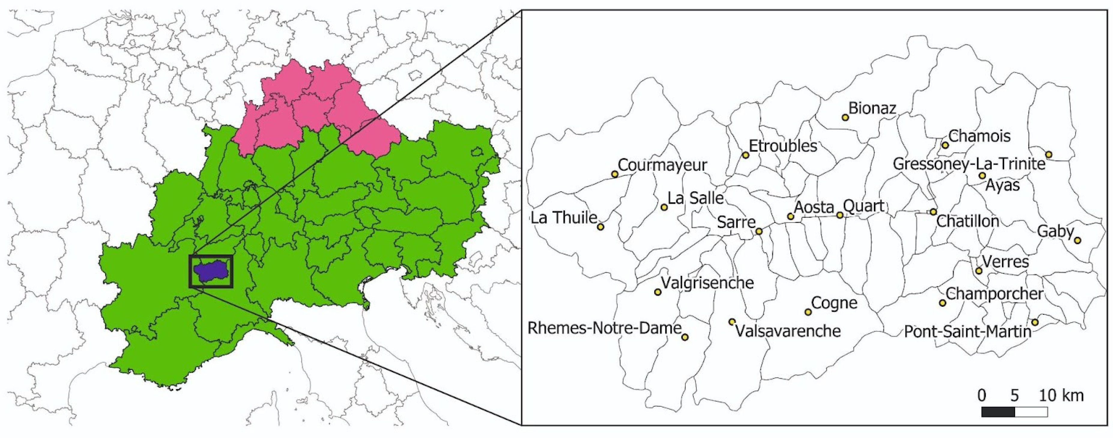
The Valle d’Aosta (Figure 1, North West of Italian Alps) is a mountainous region of about 3200 km2, and about 128,000 inhabitants surround some of the highest European massifs: Mount Blanc, Mount Rose, and the Grand Paradis. The average altitude of the whole territory is about 2100 m a.s.l. and the glaciers occupy about 5% of the total area. The main towns are all located in the Aosta plain along the main river Dora Baltea: Aosta (34,777 inhabitants), Sarre (4941), Châtillon (4844), and Saint-Vincent (4742). The majority of the Aostan population lives in the bottom valley, between 350 and 700 m a.s.l. However, some famous tourist destinations are located at high elevations: Courmayeur (1224 m a.s.l.), Valtournenche (1528 m a.s.l.), and Cogne (1524 m a.s.l.).
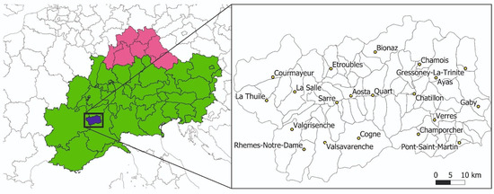
Figure 1.
On the (left), an overview of the regions of the Alpine Space cooperation area (in green) and of the EUSALP macroregion (green + magenta areas). On the (right), detail of the Aosta Valley municipalities.
The climate of the region is typically alpine, with cold winters and short summers. Temperatures vary significantly within the territory, due to the big altitude differences. From a geological point of view, the Pennidic Domain covers most of this territory and includes a broad set of rocks of originally different geological genesis and paleogeographic positions, later deformed during the orogenesis [42].
The current energy objectives of the Valle d’Aosta region are described in the Regional Environmental and Energy Plan [43] and the Monitoring Report of the following plan [44]. These plans already considered GSHPs as a low-carbon energy source to be promoted; however, planning tools for this resource still missed before this study.
2.2. Study Area Input Data and Relevant Assumptions
For the spatial financial assessment of closed-loop GSHP potential in Valle d’Aosta the main data used are listed below:
- Digital Surface Model (DSM) at 2 × 2 and 0.5 × 0.5 m of spatial resolution (source: GeoBrowser of the Region [45]);
- Digital Terrain Model (DTM) at 2 × 2 and 0.5 × 0.5 m of spatial resolution (source: GeoBrowser of the Region [45]);
- Estimated thermal demand of the residential buildings in kWh/m2/a and MWh/a [36];
- Average solar radiation (see Section 3.3) from DSM, DTM, and Albedo and Linke turbidity data derived from SODA [46];
- PV hourly profile derived from the Renewable Ninja project [47] (see Section 3.3);
- A survey was proposed in the Valle d’Aosta Region for the collection of average values for the financial and economic analysis including HPs, oil boilers, gas boilers, ACS costs and maintenance costs; electricity, oil and gas costs; gas and oil lower heating values. The results of the survey are reported in Appendix B.
In the proposed calculations, the sizing of BHE fields did not consider the available space in the area of the pertinence of the building, since this data was not available, nor the interferences among neighbouring GSHP systems. Further details on the sizing procedure and the input data are reported in Section 3.1 and Appendix A
Lastly, it is worth mentioning that the assumptions for this study were elaborated and successfully applied within the Interreg Alpine Space project (Near-surface Geothermal REsources in the Territory of the Alpine space (GRETA). Major details on the Greta Project can be found at the following website https://www.alpine-space.eu/projects/greta/en/home (accessed on 11 November 2021).
3. Methods
This study addresses the economic and financial feasibility of the use of GSHPs for providing heating and DHW for the whole residential building stock of the Italian region Valle d’Aosta. As mentioned in Section 1, this analysis was performed starting from an estimate of the thermal demand that was conducted on each of the 41,700 buildings of this region, based on a number of relevant building characteristics (for detail, see Ref. [36]).
The performances of the GSHPs were compared with traditional systems for heating/cooling and domestic hot water in four different scenarios able to consider the presence of national subsidies [48] and rooftop PV systems for electricity production (see Section 1.2). For the financial comparisons, the Levelized Cost of Energy (LCOE) [49] and the Discounted Payback Period (DPP) [8] were used as indicators:
where Et (kWh) is the amount of thermal energy produced in year t; It (€) investment costs in year t; O&Mt (€) are the operation and maintenance costs in year t; Ft (€) is the fuel costs in year t; (1 + r)−t is the discount factor for year t (at constant interest rate r); n is the fixed lifetime for a new GSHP plant; Rt (€) is the net revenue or savings for the k-th year; Ext (€) is the net expenditure for the k-th year; y is the smallest number of years for which Equation (2) is valid; Itcom (€) is the investment at year t that consider the difference between GSHP and other technologies (further details in the subsequent sections).
Indeed, these two indicators were used to investigate two different aspects, namely the average cost to produce one thermal energy unit (LCOE, €/kWh) and the length of the period needed to recover the higher investment needed for GSHPs compared to conventional heating technologies (DPP, years).
In order to highlight the implemented methodology for each building within the case study and to show how Equations (1) and (2) were implemented:
- Section 3.1 describes the load curves that were implemented for the financial analysis necessary for the dimensioning of the tested technologies (GSHP, gas/oil boiler and ACS plants) for the four considered scenarios;
- Section 3.2 describes the calculation of the It (investment costs) term in Equations (1) (LCOE) and (2) (DPP) for the four scenarios;
- Section 3.4 describes how to calculate Rt − Ext (operation and maintenance costs and net expenditure, respectively) and Itcom (investment at year t that consider the difference between GSHP and other technologies) in Equation (2) for the four scenarios. Moreover, Section 3.4 briefly presents all the inputs for Equations (1) (LCOE) and (2) (DPP).
Appendix B reports the market and maintenance costs for GSHPs, gas and oil boilers, and ACS. This input data was collected through a questionnaire in the framework of the GRETA project and the results were used as input data for the estimation of investment and operational and maintenance costs. All the analyses mentioned in this manuscript were carried out using the Python programming language [50].
3.1. Thermal Loads and BHE
Thermal loads of buildings were derived from the work of [8], related to a sensitivity analysis on the effect of building type and schedule, insulation level, and climate on the thermal loads (heating and cooling peak load and yearly need) resulting from dynamic energy simulations performed with TRNSYS [51,52]. In the study carried out in [8], three building types were considered: a detached house (residential), the town hall of a small village (office), and a hotel. These three building types are characterized by different usage schedules, different set points, depending on the comfort requirements, and different internal heat gains (e.g., much higher for offices). For each of these three building types, two different levels of insulation were considered: poor insulation typical of the 1960s (e.g., with an external wall transmittance of 1.60 Wm−2K−1) and good insulation typical of buildings of the last decade (e.g., with an external wall transmittance of 0.28 Wm−2K−1). The simulation carried out in [8] considered six climate zones, using a modified version of the ranges of heating/cooling degree days [53]. Weather reference datasets of one city for each of these zones were chosen, namely Sevilla, Bologna, Lisbon, Belgrade, Berlin, and Stockholm. For each combination—building typology (typ), climatic zone (cli), insulation (ins)—three load curves were generated (heating, cooling, domestic hot water).
In this study, starting from the data generated in Ref. [8], were considered only the load curves related to Berlin (considered as representative of zone E) and Stockholm (zone F), since these are representative of the climate of Valle d’Aosta [53]; moreover, only residential buildings were considered in this analysis, which onlyaccount for the large majority of the building stock. The selected load curves were normalized (Equation (3)) to estimate installation and operation costs for the four considered scenarios, as depicted in the subsequent sections (i.e., Section 3.2, Section 3.3, and Section 3.4).
where (kW) (or simply in Section 3.2) represent the normalized load curve for the selected building typology (typ—residential), the selected climatic zone (cli—E or F), and the selected insulation (ins); (kW) is the load curve derived from Ref. [8] for selected typ, cli, and ins; whereas (kW) is the peak of the selected load curve. Specifically, load curves were processed to derive the inputs for the ASHRAE sizing method for BHE fields. The method relies on the assumption that the thermal alteration of the heat carrier fluid is the sum of three contributions, namely the yearly average thermal load (W), the highest monthly average thermal load (W) (usually, it is January for heating and July for cooling in the Boreal hemisphere, and vice versa for the Austral one), and the peak thermal load (W). The length of BHEs needed for heating is therefore given by the following formula:
where , , and are the values of the thermal resistance of the ground (mK/W) calculated for the annual, the maximum monthly, and the peak thermal loads, respectively, assuming a duration of 10 years, 1 month, and 6 h of these stimuli; (mK/W) is the thermal resistance of the borehole; (°C) is the initial temperature of the ground; and (°C) are the minimum fluid temperatures at the inlet and the outlet of the borehole (i.e., a design constraint); and (°C) is the “temperature penalty” due to neighbouring boreholes in a BHE field and depends on the field geometry. Further details on the ASHRAE method are reported in Refs [8,39].
An exhaustive description of procedures for BHE sizing is not within the scope of this manuscript. Indeed, as stated in Section 1.2, the scope of this study is to present an assessment of the economic and financial feasibility of GSHPs for supplying the whole residential building stock of the Italian region Valle d’Aosta. In particular, all the geographically dependent data were retrieved from the geographic information database of the GRETA project [54], whereas other information on the calculation of the BHE length can be found in Appendix A, point 6.
3.2. Calculation of the Investment Cost It and of Et
The investment cost It is explicitly mentioned in Equation (1) and implicitly included in Equation (2) (see Section 3.4). The first required step for the calculation of the investment cost is the plant dimensioning and the generation of specific load curves for each of the over 40,000 buildings analyzed. In doing this, the normalized load curves described in Section 3.1 were used as the base for these calculations. In particular, the following general equations were applied.
where P(t) (kW) is the i-th load curve generated for each building (each building has three load curves for heating, cooling and domestic hot water, respectively); Pmax (kW) is the peak power for the j-th building, Pnorm(t) (kW) is the normalized load curve selected according to the building typology, climatic zone, and insulation; E (kWh) the total energy demand for each j-th building, and T = 8760 h is the duration of one year.
For the application of Equations (4) and (5), the total energy demand for each j-th building (E), the climatic condition, and the insulation typology were extracted from the data generated according to the procedure described in [36].
Considering the reduced data availability (see Section 5 and Section 6) and the number of buildings analyzed, the Pmax value calculated for the heating load curve was supposed to be equal to the installed capacity for heating and DHW. Whereas the Pmax retrieved for the cooling load curve was the input data for the calculation of the investment cost of ACS.
In particular, the data collected in Appendix B in Table A1, Table A2, Table A3 and Table A4 were used to derive regression laws (Equation (6)) to relate the installed capacities to market prices of geothermal HPs, gas/oil boilers, and ACS.
In Equation (6), the Itteq (€) value represents the investment cost for the different technologies (tec), C (kW) is the installed capacity, and (€/kWk) are the estimated coefficients of the regression law.
Data from Appendix B comes from a survey collected in March 2018 in the Valle D’Aosta region. Considering the strong non-linearity of costs vs. capacity for GSHPs, a 5th degree polynomial law was identified after a trial ad error procedure. This study considered only the capacities in the range given in Appendix B. On the other hand, a linear correlation (1st degree polynomial) cost law was identified for the ACS and the two boilers typology.
Equation (6) alone was used to calculate the It value of gas/oil boilers and ACS; on the other hand, the estimated investment costs for the GSHP also included the cost related to the borehole heat exchangers (BHE) that was calculated separately, performing a BHE sizing with the ASHRAE method for each of the about 40,000 buildings analyzed. The BHE field size (number and depth) depends on the site-specific ground thermal properties, on the load curves (Equations (3)–(5)) and BHE specific parameters (see Section 3.1).
Equation (7) reports the total investment costs for GHSP ():
where IBHE (€) is the BHE cost calculated by multiplying the unitary BHE length cost (150 €/m) for the estimated BHE length. Moreover, GSHP costs were further increased (Equation (7) parameter α) to consider that the installation can play an important role in the final investment cost (see Appendix A point 9 and [30]). This further increase was introduced to avoid an underestimation of the GSHP costs.
Lastly, in scenarios 1 and 3, which include subsidies, the following Equation (8) was applied for the estimation of the investment costs for GSHPs with the support of subsidies (expressed by β in Equation (8)). In Equation (8), we set β = 0.6 (see Annex 1 point 10).
Lastly, in the application of Equation (1), the term Et is always the same and it is equal to the total amount of heating and cooling produced in each considered building. The calculation of Et is equal to the energy E mentioned in Equation (5).
3.3. O&Mt and Ft Calculation for the Four Scenarios
The calculation of Equation (1) requires the estimation of the operation and maintenance costs for all the involved technologies and scenarios. These costs include the energy (fuel) necessary to run the plants, the annual maintenance cost of the plants, and further hypotheses to meet the requirements of the scenario (e.g., the inclusion of a PV plant for electricity production). It is worth noting that the parameters mentioned in the subsequent equations are listed in Appendix A.
The maintenance costs were derived from a similar approach described in Equation (6) using the data collected by the survey (Equation (9)). In particular, the same considerations due to the lack of linearity in the GSHP data still apply in Equation (9) (further details in Section 3.2), which was calculated for each technology (tec).
The calculation of the fuel costs was carried out, considering the load curves described in Equations (3)–(5). Equation (10) was applied to calculate the gas fuel costs for gas boilers:
In Equation (10), the units of measurement are kWh for , €/Sm3 for , MJ/Sm³ for the gas lower heating value (). In particular, the gas price is not supposed to be dependent on the consumption.
Equation (11) was applied to calculate the oil fuel costs for oil boilers:
In Equation (11), the units of measurement are kWh for , €/l for , MJ/Kg for , Kg/m3 for oil density . Like for gas, the oil price is not supposed to be dependent on consumption.
Equation (12) was applied for the calculation of electricity costs for the ACS, which was introduced in the four scenarios in combination with boilers to cover the cooling demand:
In Equation (12), the is expressed in electrical kWh; for this reason, it needs to be converted to electricity kWh, utilizing the cooling seasonal performance factor (dimensionless). The electricity unit price (€/kWh) is assumed to be nondependent on the consumption.
Equation (13) was applied for the calculation of electricity costs for the GSHP in scenarios without a coupled PV plant.
In Equation (13), the units of measurement for the heating and DHW demand and the second integral (cooling demand) are expressed in thermal kWh, and were converted to electrical kWh through the respective SPF values ( and ). As with ACSs, the electricity unit price (€/kWh) is assumed to be not dependent on the demand.
Equations (14)–(16) were implemented for the calculation of GSHP electricity cost in the scenarios including a coupled rooftop PV plant.
Equation (14) was implemented to calculate, for each building, a PV electricity load curve exploiting a unit load curve (the time series of , i.e., the kWh produced per hour, per kW installed) that was retrieved using the tool provided by the Renewable Ninja project [47].
The available roof area for PV plants was calculated for each building, starting from the Digital Surface Model (DSM) of the region and including both terrain and building roof quotes. The GRASS GIS r.sun module [55] was used to estimate the beam solar irradiation over the whole year, in clear-sky conditions, which was calculated from Linke atmospheric turbidity and albedo datasets (further details in Appendix A). For this study, the potentially available PV areas that were considered to be suitable are only those where the annual direct irradiation on the roof area exceeds the 75th percentile of the distribution of the beam solar irradiation. For these roof areas (APV in Equation (14)), high performance PV systems were hypothesized, applying a conversion factor of . Finally, only the resulting PV systems with at least 1 kW were taken into account. As a consequence, the number of buildings considered in scenarios 2 and 3 is slightly smaller if compared with the original number of scenarios in 1 and 4.
Starting from the electrical demand curve created in Equation (14) (for each building), the coverage of such demand with the PV plant was assessed and a new electricity demand curve (Equation (15)) was derived, assuming no electrical storage unit. Therefore, the PV system covers the demand of the heat pump only when it produces at least the same power; otherwise, electricity is drawn from the grid to cover the demand of the heat pump, or part of it. To include the cost of the investment connected with a further PV plant, the PV electricity is supposed to have a unit cost equal to the term in Equation (16) (further details in Appendix A).
3.4. Inputs of the Analysis
Equation (2) is normally used to calculate the profitability of an investment. In the case of a building energy refurbishment, this does not produce any direct revenue for the householders, but the operational savings of GSHPs compared to (fossil fuel) boilers can be considered as a revenue that repay the higher investment required. Equation (2) provides an indication of the amount of time (paybak time) that is, on average, needed to reach a break-even point from undertaking the initial major expenditure for the installation of GSHPs.
Considering this, in the four scenarios, the yearly difference between the revenues and the expenditures in Equation (2) is given by the difference between the sum of fuel costs and O&M cost for traditional technology and the sum of fuel costs and O&M for GSHP, whereas the investment cost mentioned in Equation (2) is given by the difference between the investment costs of the GSHP plant (supposed higher) and the investment cost of traditional technologies.
Equations (6)–(16) provide all the inputs for the application of Equations (1) and (2) for almost 40,000 buildings analyzed in this study. In particular, Table 1 depicts the inputs for the calculation of the LCOE (Equation (1)) for the four GSHP-related scenarios, for the combination of gas boiler and ACS, and the combination of oil boiler and ACS. Table 2 and Table 3 depict the inputs for the calculation of the DPP related to the comparisons of the four GSHP-related scenarios with gas boiler and ACS and the comparisons of the four GSHP-related scenarios with oil boiler and ACS, respectively.

Table 1.
Input data calculated according to Equations (3)–(16) for the spatial explicit LCOE assessments.
Table 2.
Input data calculated according to Equations (3)–(16) for the spatial explicit DPP assessments. The inputs are related to the comparisons between GSHP with a gas-boiler/ACS system.
Table 3.
Input data was calculated according to Equations (3)–(16) for the spatial explicit DPP assessments. The inputs are related to the comparisons between GSHP with an oil-boiler/ACS system.
Lastly, the proposed scenarios included the possibility to consider public subsidies (i.e., Conto Termico in Italy). The subsidies, reported in Ref. [41], when applied in Scenarios 1 and 3, considered 65% of the whole closed-loop system capital cost subtracted from the overall capital cost estimated. No other loan grant/subsidies or discount over time were considered.
4. Results
To evaluate the suitability of the near-surface geothermal resource to cover the heating and cooling demand in the Valle D’Aosta region, spatially explicit analyses were performed over the whole residential building stock of the smallest Italian Region. Within this analysis, all the hypotheses and equations described in Section 3 and in Appendix A were applied. In particular, the financial analysis is reported employing the technology-related LCOE and DPP values for the four following scenarios.
In Figure 2, Table 4 and Table 5 synthetically describe the results of the calculations carried out for each residential building of the Valle d’Aosta Region.

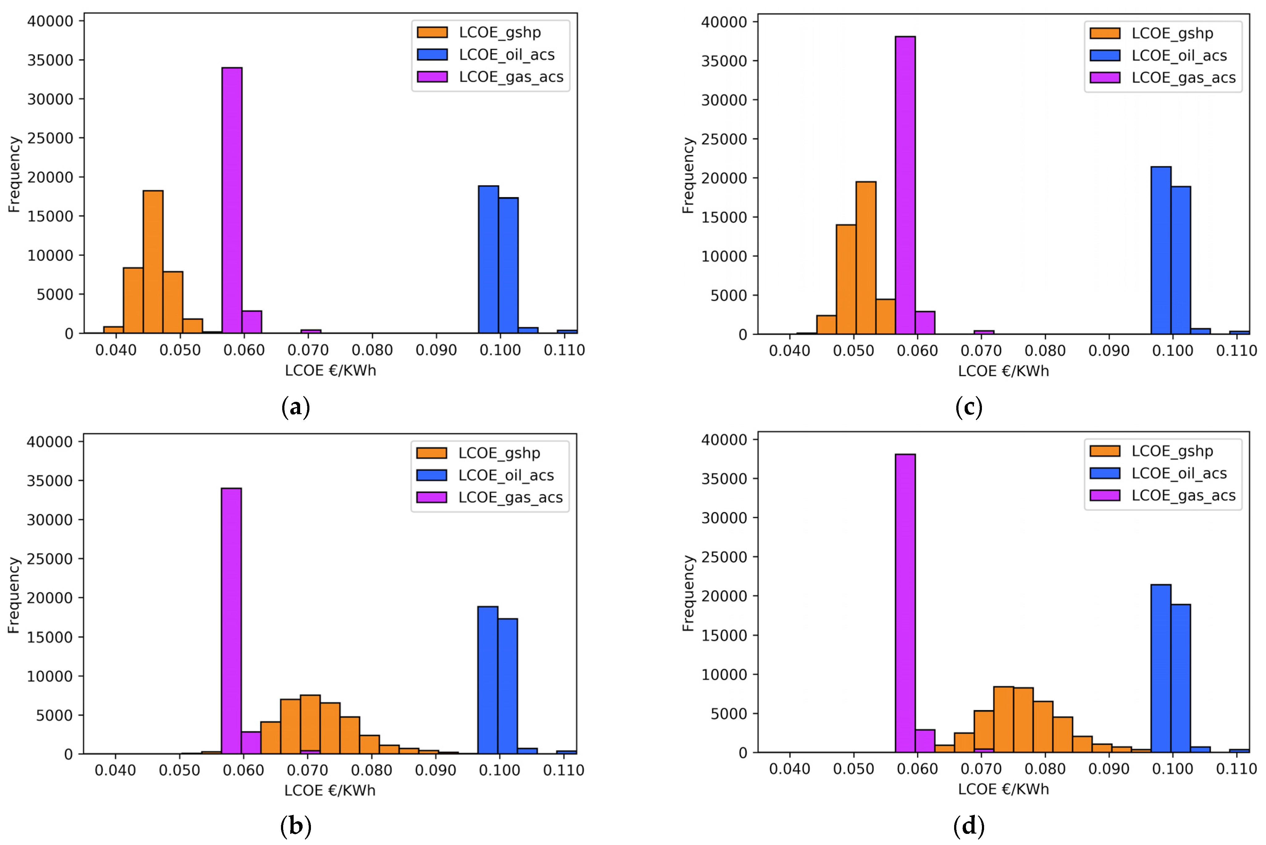
Figure 2.
Valle d’Aosta closed-loop LCOE histograms for the scenarios including closed-loop ground source heat pumps; gas boiler and air conditioning system (gas_acs); oil boiler and air conditioning system (oil_acs): (a): Scenario 1, including solar rooftop PV systems and subsidies. (b): Scenario 2, including solar rooftop PV systems, excluding subsidies. (c): Scenario 3, excluding solar rooftop PV systems, including subsidies. (d): Scenario 4, excluding solar rooftop PV systems and subsidies.
Table 4.
Univariate statistics for LCOE data of the Valle d’Aosta region, considering the following comparisons between closed-loop HP plants and gas boiler and ACS (gas_acs), oil boiler and ACS (oil_acs), and the four closed-loop scenarios.
Table 5.
Average values of Discounted Payback Period (DPP) of GSHPs compared to an oil/gas boiler with an ACS in the four scenarios (with/without subsidies; with/without roof PV system).
Figure 2 depicts the LCOE histograms of the four considered scenarios. In these histograms (Figure 2a–d), the LCOE distribution of gas/oil boilers and ACS are fixed, whereas the GSHP-related one (orange columns) varies depending on the presence of PV and/or subsidies. A clear effect of subsidies for the GSHP LCOE can be observed by comparing Figure 2b–d (scenarios 2 and 4, respectively) and Figure 2a–c (scenarios 1 and 3, respectively). As expected, gas boilers + ACS turns out to be always more convenient than the oil boiler + ACS. On the other hand, Figure 2 shows that the installation of a rooftop PV system coupled with a GSHP only slightly reduces the LCOE values of GSHPs, as one can observe comparing Figure 2b (scenario 2) and Figure 2d (scenario 4), respectively, with Figure 2a (scenario 1) and Figure 2c (scenario 3). As expected, the conjunct application of subsidies and the rooftop PV system is the most economically convenient solution.
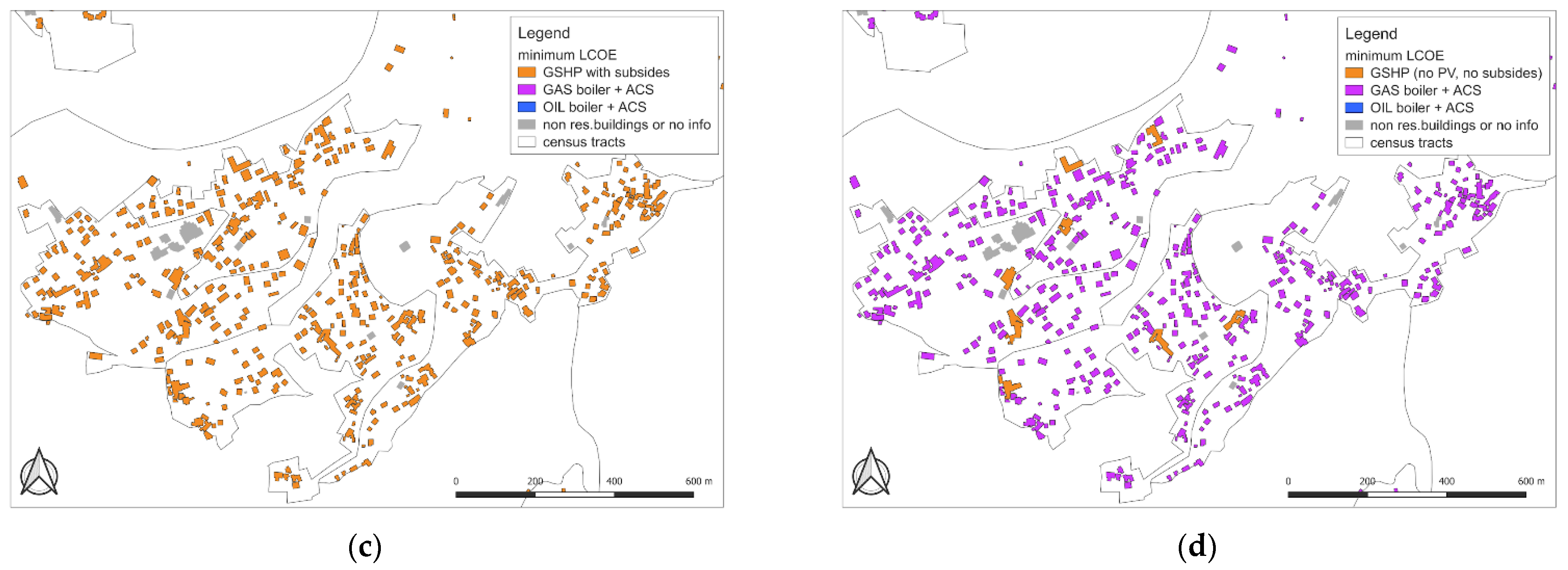
Figure 3a–d show, in a spatially-explicit way, the minimum LCOE for GSHP, oil/gas boilers, and ACS over a spatial subset of the study area (the municipality of Aymavilles) for the four Scenarios. In particular, Figure 3b,d shows that, without subsidies, the GSHP is the most financially feasible solution for only a minor part of residential buildings. In particular, scenarios 2 and 4 feature very similar results, whereas Figure 3a,c shows that the application of subsidies plays a key role in the financial feasibility of the domestic closed-loop GSHP.
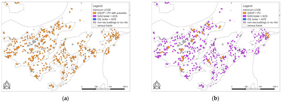
Figure 3.
Maps on the comparison between the minimum values of LCOE per building for four technology scenarios in Valle d’Aosta (examples from Aymavilles municipality): (a): GSHP Scenario 1, with both subsidies and rooftop photovoltaic systems. (b): GSHP Scenario 2, without subsidies and with rooftop photovoltaic systems. (c): GSHP Scenario 3, with subsidies and without rooftop photovoltaic systems. (d): GSHP Scenario 4, without subsidies nor rooftop photovoltaic systems.
Table 4 shows univariate LCOE statistics (average value, standard deviation, skewness, and kurtosis) for the four scenarios related to closed-loop HP plants. Such a table features only one set of univariate statistics for the two combinations of gas and oil boilers with ACS, since no specific scenarios were applied to these configurations and because rooftop solar PV systems were only applied to HP plants. This means that all the prices for gas and oil boiler combinations do not change for a considered i-th building in the four scenarios proposed in Figure 2.
In the analysis of Table 4 and Table 5, it is worth mentioning that the application of the hypothesis reported in Appendix A caused the decrease of the number of the LCOE calculations related to scenarios involving rooftop PV systems. Some roof areas, where it was not possible to include PV panels (according to hypotheses formulated in point 7 of Appendix A), were excluded from the input data implemented in the spatial-explicit simulations. Table 4 provides a quantitative description of Figure 2. Fossil fuel options are characterized by a smaller standard deviation, that is, they are less affected by the spatial variability of the input data.
All distributions feature a positive skewness and are leptokurtic, that is, they are characterized by higher extreme LCOE values if compared with a hypothetical normal distribution. In particular, the LCOE distributions for closed-loop geothermal systems have a significantly higher number of extreme values compared to oil/gas boilers configurations, as one can also observe from the plots shown in Figure 2. This result can be justified considering the higher spatial variability in the closed-loop HP plants’ investment costs. Indeed, just to mention an important input for GSHP capital costs, excavation costs were separately calculated for each input record (i.e., each building) and each scenario. Considering the dependence among borehole heat exchange (BHE) length, thermal demand, and site-specific geological properties, this result is justified. Major detail on calculation hypotheses related to GSHP can be retrieved in point 6 of Appendix A.
Table 5 shows the average value for each DPP distribution and the two comparisons carried out against conventional technologies. The results displayed are consistent with Figure 2 and Table 4. In addition, DPP values of GSHPs, when compared to oil boilers + ACS, are lower than those obtained in comparison with a gas boiler and ACS configuration. Considering the higher costs of heating oil compared to gas, this result is expected. Moreover, considering a specific comparison (e.g., DPP closed-loop vs. oil_acs), we can note that DPP values follow expected patterns: DPP Scenario 4 > DPP Scenario 2 > DPP Scenario 3 > DPP Scenario 1. This result, again, highlights the contribution of rooftop PV systems and of the Italian subsidies for energy refurbishment of buildings; however, the effect of subsidies is much stronger than that of PV systems.
5. Discussion
This article reports the results of the application of spatial-based financial feasibility evaluations for the application of closed-loop GSHP systems in the Valle d’Aosta region.
The Results section showed several outputs for the study area, considering a high number of different input data with different levels of detail.
Considering all the assumptions proposed in Appendix A, it is clear that the study has some inherent limitations:
- The problems that might arise due to dense exploitation of the geothermal resource for heating and cooling (e.g., a set of inefficient plants due to reciprocal interference among adjacent systems) are not considered. All the calculations were carried out considering each building separately;
- The presence of hybrid systems (e.g., HP combined with an auxiliary gas boiler) is not considered;
- Many simplifications and assumptions were necessary to perform an analysis on more than 40,000 residential buildings. For instance, in the estimation of GSHP capital costs, installation and design costs were not directly estimated. Indeed, these specific costs were taken into account with a 40% increase in the excavation costs (see Appendix A). A previous study carried out on a Central European geographic context highlighted that the average BHE depth is about 100 m and that installation costs other than the heat pump and the borehole drilling are not negligible and are highly variable [56].
Overall, in this study, the authors are aware of the fact that some assumptions might lead to an overestimation of the GSHP capital costs. On the other hand, for this specific case study, it was not possible to carry out a case by case validation of the input data, due to data unavailability (e.g., starting from the spatial distribution of thermal demand [36]). Considering this, the level of uncertainty in the capital costs estimation is acceptable and in line with the possibilities offered by the study area’s data availability.
As reported in Ref. [36], datasets are often not available or their accessibility is limited by the data providers. Moreover, heterogeneous data granularity constitutes another major issue. A typical example of this issue is the high probability, for the same administrative area (region, province, or municipality), of having some data accessible at the building level, whereas other data is available only at the census or district level. Data abundance, resolution, and availability represents a relevant limit for the analysis itself, as well as for the accuracy of the results.
Despite this, the analyses here described can estimate, for each building, the values needed for the data processing, allowing us to reach a compromise between the number of input data and the level of detail often required by policymakers. In the Valle d’Aosta pilot area, the spatial-based approach has proven to be useful for assessing all scenarios in Section 4.
From a general point of view, the results clearly show that closed-loop GSHP installations are characterized by a higher variability in LCOE if compared to gas/oil boilers and ACS, and that this is mostly due to the dependence on site-specific soil thermal parameters.
In this pilot area, the gas-boiler and ACS combination features a clear convenience with respect to the oil-boiler and ACS combination. This is due to the high difference in fuel costs in the Italian context. The combined use of HP plants with rooftop solar PV systems is certainly able to positively influence the DPP and LCOE values of geothermal HP systems. However, the real game changer in the economic and financial analysis is the application of subsidies. From this point of view, it is worth noting that the analysis presented in the paper is related to the year 2018, when the existing subsidies scheme (Conto Termico and Ecobonus) could reach a maximum of 65% of the whole investment. In May 2020, the so-called Superbonus was introduced as an economic recovery measure to tackle the COVID-19 pandemic-related crisis. The Superbonus refunds up to 110% of the investment for energetic refurbishment of buildings; however, the authors did not consider this incentive due to its short and unpredictable duration, whereas Ecobonus and Conto Termico have been in force for more than 10 years.
6. Conclusions
This manuscript synthetically reports the results of the spatial evaluation of the financial and economic analyses of GSHPs to cover the heat demand of the residential building stock of the Italian region Valle d’Aosta. The aim is to provide more insight for decision-makers, i.e., energy policymakers, regional public authority, energy managers, etc., on how to integrate the exploitation of shallow geothermal sources into energy plans and strategies from a financial point of view.
The main findings are hereby summarized:
- The procedure and the methodology identified in this manuscript can be potentially replicated in other case studies. However, it is possible to conclude that a spatially explicit analysis (such as the one carried out in this manuscript) of the economic/financial feasibility of GSHP needs a robust set of input data;
- In particular, the followings inputs should be collected (or estimated from other sources of information):
- ○
- The geological properties of the study area;
- ○
- The hydraulic characteristics of the ground;
- ○
- The technical features of the considered buildings (i.e., thermal insulation, etc.);
- ○
- The load curve, which is the hourly thermal demand (heating and cooling) of the buildings;
- ○
- The thermal need required by the activities carried out within the buildings (different for residential, hotel, office, industrial processes, etc.);
- ○
- The investment, maintenance, and operative costs of the alternative technological solutions to perform effective economic/financial comparisons;
- ○
- All of the aforementioned information should be collected using redundant and robust methods, against uncertainties, to improve the reliability of the analysis;
- ○
- All of the aforementioned points should be spatially distributed and assessed to create the conditions for fast data integration (e.g., join of information).
- The method is affected by data abundance, data structure, and granularity. Input and easy-to-use data are needed to perform more reliable and frequent estimations at the building level.
- Due to the high variability of the GSHP potential, a spatial-based assessment of their economic and financial feasibility can support decision-makers in exploiting and incentivising this resource in a more effective way to increase its convenience. Subsidies can make a difference in the convenience of GSHP plants. In the author’s opinion, they are important in the transition phases, in which strong subsidies can enhance the spread of cleaner technologies.
This study does not consider the environmental benefits related to the massive implementation of GSHPs (e.g., in Ref. [8], an energy demand reduction ranging from 33 to 75% and a carbon dioxide reduction ranging from 27 to 56% was estimated in Italy). This specific aspect can be considered in the future development of this research, together with a sensitivity analysis to highlight the minimum level of subsidies that would enable GSHP penetration.
Author Contributions
Conceptualization, A.N., V.D., S.P., R.A.E.P., P.Z.; methodology, A.N., V.D., S.P., R.A.E.P., A.C., P.Z.; software, A.N., V.D., S.P., R.A.E.P., P.Z.; visualization, A.N., V.D., S.P., R.A.E.P., P.Z.; writing—original draft preparation, A.N., V.D., S.P., R.A.E.P., A.C., P.Z.; writing—review and editing, A.N., V.D., S.P., R.A.E.P., A.C., P.Z. All the authors revised the manuscript. All authors have read and agreed to the published version of the manuscript.
Funding
This research work was conducted within the GRETA project and supported by the European Regional Development Fund (ERDF) through the Interreg Alpine Space Programme (ASP172).
Acknowledgments
This research work was conducted within the GRETA project and supported by the European Regional Development Fund (ERDF) through the Interreg Alpine Space Programme (ASP172). Moreover, we thank the anonymous reviewers for their careful reading of our manuscript and their many insightful comments and suggestions.
Conflicts of Interest
The authors declare no conflict of interest.
Appendix A
Due to the lack of spatially distributed information, computational constraints, and simplifications needed to effectively address the complex issues, the described analysis required some hypotheses and assumptions. The most relevant are described in the following paragraphs:
- The whole thermal demand was satisfied with HP plants (i.e., no auxiliary boilers were included in the analysis). Particularly, HP plants for heating, cooling, and domestic hot water were compared to a coupled natural gas boiler and air conditioning systems (ACS) and a coupled heating oil boiler and ACS. This assumption was made since hybrid systems (HP and boiler) are not available in the market for ground source heat pumps, therefore customized systems would be necessary.
- In these comparisons, the main working hypothesis was that HP plants are characterized by higher investment costs and lower annual costs [15], concerning the aforementioned boiler plus ACS.
- For the geothermal HP plants, a lifetime of 27 years [57] and 20 years was considered, according to the average lifetime of conventional boiler equipment [58] for other plants (gas and oil boilers).
- To evaluate the borehole heat exchanger (BHE) length, the ASHRAE method was used.
- Raster data on thermal conductivity, thermal capacity, thermal diffusivity, and ground temperature were provided by the GRETA project [54].
- The following parameters and assumptions were applied for the application of the ASHRAE [39] method for BHE:
- Peak hourly ground load, monthly ground load, yearly average ground load necessary for BHE dimensioning were estimated for each building considering the annual thermal demand and the normalized hourly profile according to [8];
- Fluid thermal heat capacity [J.kg−1K−1] = 3930 (propylene glycol 25%, see Ref. [59]);
- Fluid total mass flow rate per kW of peak hourly ground load [kg.s−1.kW−1] = 0.025 (this value was set assuming a temperature difference of 3 °C (see VDI 4640, Ref. [60]);
- Max/min heat pump inlet temperature [C] = -2.0 (the freezing point of PG25% is −10 °C, according to Ref. [61]);
- Borehole radius [m] = 0.075;
- Pipe inner radius [m] = 0.0137 (32 mm HDPE pipes);
- Pipe outer radius [m] = 0.0167 (32 mm HDPE pipes);
- Grout thermal conductivity [W.m−1.K−1] = 2.0 (typical conductivity value for geothermal grouts, see Ref. [61]);
- Pipe thermal conductivity [W.m−1.K−1] = 0.42 (HDPE pipes);
- Center-to-center distance between inlet and outlet pipes inside a BHE [m] = 0.0511;
- Internal convection coefficient [W.m−2.K−1] = 1000 [40];
- In the application of the ASHRAE method, a single borehole was considered, since the aim was only the estimation the cost of the excavation;
- The length of the BHE was increased by 3% to take into account the possible thermal interference among different BHEs, as this is was an intermediate value between 1 (no short-circuit) and 1.05 (strong short-circuit).
- One kW for seven square meters is the conversion factor implemented in Equation (14). Because we consider a 15% [62] average efficiency of a PV panel, and as we consider that a typical peak value is 1000 W/m2 on a terrestrial surface facing the sun on a clear day around solar noon at sea level, to obtain 1 kWp, the installed measures are necessary, 1/0.15 = 6.667 m2, so at least 7 m2. Given the availability of Digital Surface Model (DSM) data for the territory of Valle d’Aosta, including both terrain quotes and building roof ones, the GRASS GIS r.sun module [55] was used to estimate the beam solar irradiation over the whole year in clear-sky conditions. Roofs were considered as covered by a solar photovoltaic (PV) system (1 kW for 7 square meters) if the annual direct irradiation on the roof area was greater than the 75th percentile of the distribution of the beam solar irradiation. In particular, the main input data involved in the r.sun module computation were:
- An elevation raster map;
- An aspect raster map (map with the direction that slopes are facing counterclockwise from East: 90 degrees is North, 180 is West, 270 is South, 360 is East [63]);
- The Linke atmospheric turbidity raster map that was achieved interpolating Linke atmospheric turbidity data from the SoDa Service (http://www.soda-pro.com/—accessed, accessed on 11 November 2021), albedo data calculated by interpolating albedo data distributed by the SoDa Service, and horizon raster maps (step 5 sexagesimal degrees).
- Solar PV systems were implemented within the simulations and their contribution was evaluated by employing an LCOE of €0.09 for each produced kWh [64]. In this way, the solar PV investment cost was taken into account, even if it was not directly considered in the computations. In addition, sun hourly profiles used for the estimation of the produced energy by solar PV plants were gathered from the renewable ninja website (further details in [47]). Capital costs and annual costs of geothermal HP plants were obtained through regressions performed over surveyed data or from available references [37].
- Since the high variability and uncertainty of the analyzed cases in terms of building thermal demand, insulation, plant configuration, etc., (as depicted in [30]) it was not possible to calculate the plant installation cost of each component of the geothermal system. Therefore, to avoid unrealistic low GSHP capital cost estimations, the estimated excavation and HP costs (capital cost) were increased by 40%. This percentage is estimated from Ref. [30] to consider all the other system components that were not directly estimated in capital costs. Indeed, from Ref. [30] the costs of the heat pump and BHE account for about 60% of the cost breakdown of the GHSP system. For this reason, the estimated costs were increased by the value of 40% to obtain capital costs estimation more in line with the reference.
- The subsidies were estimated starting from the national regulation (i.e., Conto Termico in Italy) and directly subtracted from HP plant costs (i.e., they were not spread over the considered time span, since it may vary according to the plant power and the system efficiency).
- The hourly profiles of thermal demand were derived from the simulations performed by POLITO (further details in [37] and in “GRETA Project—Near-surface Geothermal Resources in the Territory of the Alpine Space—Alpine Space”, 2018) and from the estimation of the annual thermal demand for each residential building in the case study [37].
- BHE supposed unitary excavation cost equal to 150 €/m.

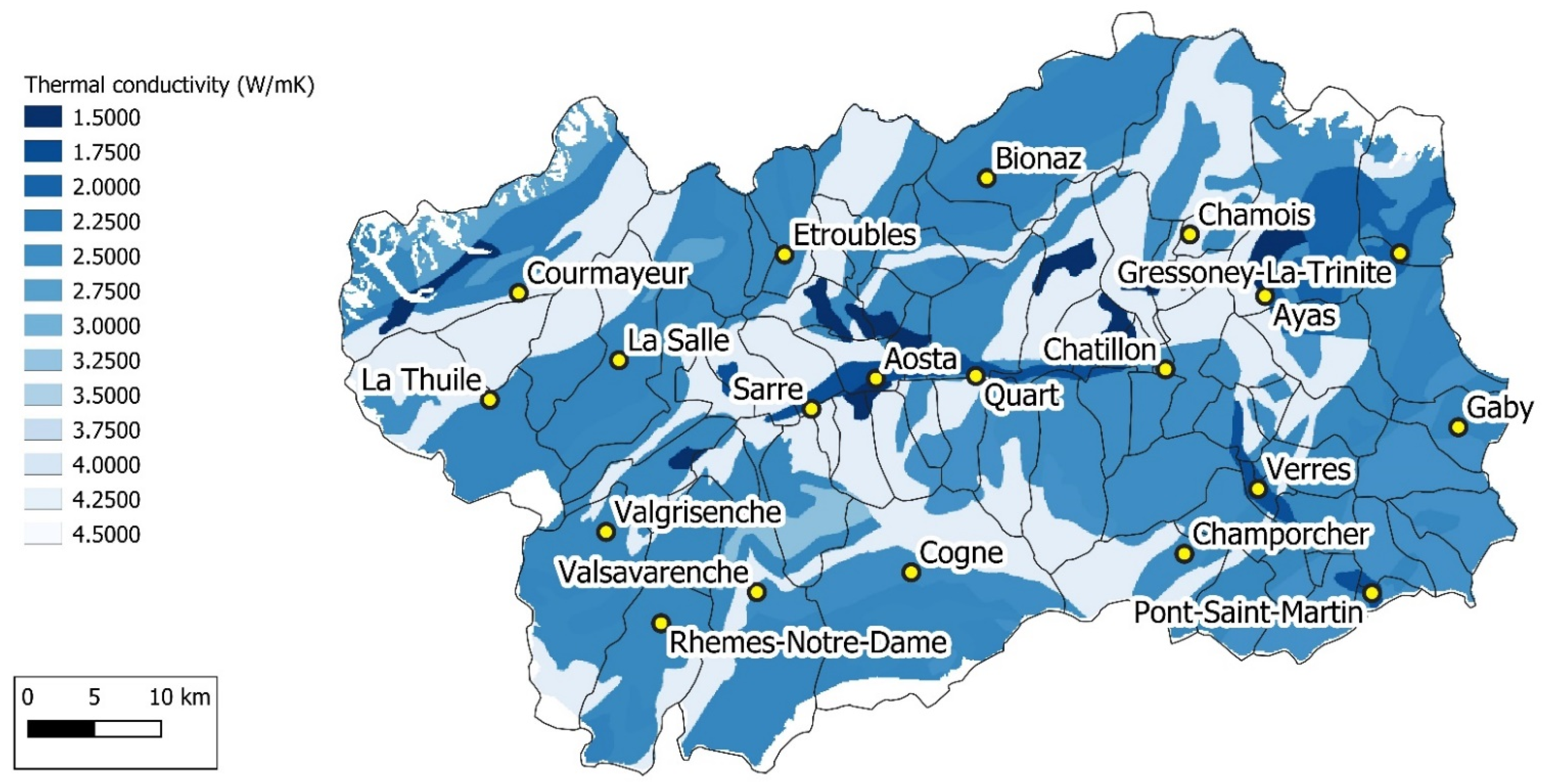
Figure A1.
Spatial distribution of the average thermal conductivity of the underground (depth up to 100 m) in the Aosta Valley. Modified from Casasso et al., 2018 [42].
Figure A1.
Spatial distribution of the average thermal conductivity of the underground (depth up to 100 m) in the Aosta Valley. Modified from Casasso et al., 2018 [42].
Appendix B
The following survey was collected in the Valle d’Aosta region for the collection of the input data related to capital, operational, and maintenance costs of the tested technologies (reference time: February 2018).
Table A1.
Heat pump cost survey.
Table A1.
Heat pump cost survey.
| Question | Thermal Power [kW] | Cost [EUR] | Annual Maintenance [EUR] |
|---|---|---|---|
| please provide five kW/cost/anno. Maintenance entries (possibly equally distributed) included in the range of 6–50 kW (heating performance). The cooling performance is supposed to be greater than 70% of the heating performance. | 7.6 | 10,176 | 91 |
| 13 | 12,305 | 177 | |
| 28.8 | 19,391 | 372 | |
| 42.8 | 25,965 | 488 | |
| 50 | 34,095 | 610 | |
| please provide five kW/cost entries (possibly equally distributed) included in the range of 51–250 kKW (heating performance). The cooling performance is supposed to be greater than 70% of the heating performance. | 57.6 | 42,112 | 792 |
| 85.6 | 51,924 | 1341 | |
| 134.6 | 45,332 | 1829 | |
| 173.2 | 53,544 | 2316 | |
| 222 | 59,699 | 2926 | |
| please provide five kW/cost entries (possibly equally distributed) included in the range of 251–600 kW (heating performance). The cooling performance is supposed to be greater than 70% of the heating performance. | 280 | 286,160 | 5320 |
| 340 | 347,480 | 6460 | |
| 400 | 408,800 | 7600 | |
| 490 | 500,780 | 9310 | |
| 560 | 572,320 | 10,640 |
Table A2.
Gas Boiler cost survey.
Table A2.
Gas Boiler cost survey.
| Question | Thermal Power [kW] | Cost [EUR] | Annual Maintenance [EUR] |
|---|---|---|---|
| please provide five kW/cost entries (possibly equally distributed) included in the range of 6–50 kW (heating performance). | 17.4 | 1780 | 91 |
| 23.8 | 1955 | 177 | |
| 32.1 | 2321 | 372 | |
| 40 | 7320 | 600 | |
| 50 | 9150 | 750 | |
| please provide five kW/cost entries (possibly equally distributed) included in the range of 51–250 kW (heating performance). | 65 | 11,895 | 975 |
| 110 | 20,130 | 1650 | |
| 150 | 27,450 | 2250 | |
| 190 | 34,770 | 2850 | |
| 240 | 43,920 | 3600 | |
| please provide five kW/cost entries (possibly equally distributed) included in the range of 251–600 kW (heating performance). | 280 | 51,240 | 4200 |
| 340 | 62,220 | 5100 | |
| 400 | 73,200 | 6000 | |
| 490 | 89,670 | 7350 | |
| 560 | 102,480 | 8400 |
Table A3.
Oil Boiler cost survey.
Table A3.
Oil Boiler cost survey.
| Question | Thermal Power [kW] | Cost [EUR] | Annual Maintenance [EUR] |
|---|---|---|---|
| please provide five kW/cost entries (possibly equally distributed) included in the range of 6–50 kW (heating performance). | 17.4 | 1780 | 91 |
| 23.8 | 1955 | 177 | |
| 32.1 | 2321 | 372 | |
| 40 | 7320 | 600 | |
| 50 | 9150 | 750 | |
| please provide five kW/cost entries (possibly equally distributed) included in the range of 51–250 kW (heating performance). | 65 | 11,895 | 975 |
| 110 | 20,130 | 1650 | |
| 150 | 27,450 | 2250 | |
| 190 | 34,770 | 2850 | |
| 240 | 43,920 | 3600 | |
| please provide five kW/cost entries (possibly equally distributed) included in the range of 251–600 kW (heating performance). | 280 | 51,240 | 4200 |
| 340 | 62,220 | 5100 | |
| 400 | 73,200 | 6000 | |
| 490 | 89,670 | 7350 | |
| 560 | 102,480 | 8400 |
Table A4.
Air conditioning system cost survey.
Table A4.
Air conditioning system cost survey.
| Question | Thermal Power [kW] | Cost [EUR] | Annual Maintenance [EUR] |
|---|---|---|---|
| please provide five kW/cost entries (possibly equally distributed) included in the range of 6–50 kW (heating performance). | 17.4 | 1780 | 91 |
| 23.8 | 1955 | 177 | |
| 32.1 | 2321 | 372 | |
| 40 | 7320 | 600 | |
| 50 | 9150 | 750 | |
| please provide five kW/cost entries (possibly equally distributed) included in the range of 51–250 kW (heating performance). | 65 | 11,895 | 975 |
| 110 | 20,130 | 1650 | |
| 150 | 27,450 | 2250 | |
| 190 | 34,770 | 2850 | |
| 240 | 43,920 | 3600 | |
| please provide five kW/cost entries (possibly equally distributed) included in the range of 251–600 kW (heating performance). | 280 | 51,240 | 4200 |
| 340 | 62,220 | 5100 | |
| 400 | 73,200 | 6000 | |
| 490 | 89,670 | 7350 | |
| 560 | 102,480 | 8400 |
Table A5.
Input data for the calculation of operational costs.
Table A5.
Input data for the calculation of operational costs.
| Technical Feature | Value |
|---|---|
| Electricity price [EUR/kWh] | 0.21 |
| Gas price [EUR/Sm3] | 0.8 |
| Heating oil price [EUR/l] | 1.4 |
| Gas lower heating value [MJ/Sm3] | 34 |
| Oil lower heating value [MJ/kg] | 40 |
References
- Laustsen, J. Energy Efficiency Requirements in Building Codes, Energy Efficiency Policies for New Buildings. IEA Information Paper. Support of the G8 Plan of Action. 2008. Available online: https://www.iea.org/reports/energy-efficiency-requirements-in-building-codes-policies-for-new-buildings (accessed on 1 November 2021).
- Pezzutto, S.; Croce, S.; Zambotti, S.; Kranzl, L.; Novelli, A.; Zambelli, P. Assessment of the Space Heating and Domestic Hot Water Market in Europe—Open Data and Results. Energies 2019, 12, 1760. [Google Scholar] [CrossRef] [Green Version]
- Pezzutto, S.; Fazeli, R.; De Felice, M.; Sparber, W. Future Development of the Air-Conditioning Market in Europe: An Outlook until 2020. Wiley Interdiscip. Rev. Energy Environ. 2016, 5, 649–669. [Google Scholar] [CrossRef]
- Polesello, V.; Johnson, K. Energy-Efficient Buildings for Low-Carbon Cities. ICCG Reflect. 2016, 47, 1–9. [Google Scholar]
- EHPA. European Heat Pump Market and Statistic Report 2017 & Stats Tool. Available online: https://www.ehpa.org/market-data/2017/ (accessed on 11 November 2021).
- Heinonen, J.; Laine, J.; Pluuman, K.; Säynäjoki, E.-S.; Soukka, R.; Junnila, S. Planning for a Low Carbon Future? Comparing Heat Pumps and Cogeneration as the Energy System Options for a New Residential Area. Energies 2015, 8, 9137–9154. [Google Scholar] [CrossRef] [Green Version]
- Bayer, P.; Saner, D.; Bolay, S.; Rybach, L.; Blum, P. Greenhouse Gas Emission Savings of Ground Source Heat Pump Systems in Europe: A Review. Renew. Sustain. Energy Rev. 2012, 16, 1256–1267. [Google Scholar] [CrossRef]
- Rivoire, M.; Casasso, A.; Piga, B.; Sethi, R.; Rivoire, M.; Casasso, A.; Piga, B.; Sethi, R. Assessment of Energetic, Economic and Environmental Performance of Ground-Coupled Heat Pumps. Energies 2018, 11, 1941. [Google Scholar] [CrossRef] [Green Version]
- Lund, J.W.; Boyd, T.L. Direct Utilization of Geothermal Energy 2015 Worldwide Review. Geothermics 2016, 60, 66–93. [Google Scholar] [CrossRef]
- Staffell, I.; Brett, D.; Brandon, N.; Hawkes, A. A Review of Domestic Heat Pumps. Energy Environ. Sci. 2012, 5, 9291–9306. [Google Scholar] [CrossRef]
- Lund, J.W. Direct Utilization of Geothermal Energy. Energies 2010, 3, 1443–1471. [Google Scholar] [CrossRef]
- Florides, G.; Kalogirou, S. Ground Heat Exchangers—A Review of Systems, Models and Applications. Renew. Energy 2007, 32, 2461–2478. [Google Scholar] [CrossRef]
- Kavanaugh, S.; Gilbreath, C.; Kilpatrick, J. Cost Containment for Ground-Source Heat Pumps, Final Report. Available online: https://bit.ly/2XaC0xH (accessed on 19 May 2020).
- Petit, P.J.; Meyer, J.P. Economic Potential of Vertical Ground-Source Heat Pumps Compared to Air-Source Air Conditioners in South Africa. Energy 1998, 23, 137–143. [Google Scholar] [CrossRef]
- Shonder, J.A.; Martin, M.A.; Hughes, P.J.; Thornton, J. Geothermal Heat Pumps in K-12 Schools: A Case Study of the Lincoln, Nebraska Schools. Available online: https://digitalcommons.unl.edu/usdoepub/30/ (accessed on 19 May 2020).
- Self, S.J.; Reddy, B.V.; Rosen, M.A. Geothermal Heat Pump Systems: Status Review and Comparison with Other Heating Options. Appl. Energy 2013, 101, 341–348. [Google Scholar] [CrossRef]
- Chiasson, A.D.; Yavuzturk, C.; Talbert, W.J. Design of School Building HVAC Retrofit with Hybrid Geothermal Heat-Pump System. J. Archit. Eng. 2004, 10, 103–111. [Google Scholar] [CrossRef]
- Chiasson, A.D. Greenhouse Heating with Geothermal Heat Pump Systems. Available online: https://bit.ly/3bPanQ2 (accessed on 11 November 2021).
- Chiasson, A. Final Report Life-Cycle Cost Study of a Geothermal Heat Pump System BIA Office BLDG. Available online: https://bit.ly/2LEA4IF (accessed on 19 May 2020).
- Esen, H.; Inalli, M.; Esen, M. Technoeconomic Appraisal of a Ground Source Heat Pump System for a Heating Season in Eastern Turkey. Energy Convers. Manag. 2006, 47, 1281–1297. [Google Scholar] [CrossRef]
- Esen, H.; Inalli, M.; Esen, M. A Techno-Economic Comparison of Ground-Coupled and Air-Coupled Heat Pump System for Space Cooling. Build. Environ. 2007, 42, 1955–1965. [Google Scholar] [CrossRef]
- Badescu, V. Economic Aspects of Using Ground Thermal Energy for Passive House Heating. Renew. Energy 2007, 32, 895–903. [Google Scholar] [CrossRef]
- Hanova, J.; Dowlatabadi, H. Strategic GHG Reduction through the Use of Ground Source Heat Pump Technology. Environ. Res. Lett. 2007, 2, 044001. [Google Scholar] [CrossRef]
- Dickinson, J.; Jackson, T.; Matthews, M.; Cripps, A. The Economic and Environmental Optimisation of Integrating Ground Source Energy Systems into Buildings. Energy 2009, 34, 2215–2222. [Google Scholar] [CrossRef]
- Zhu, Y.; Tao, Y.; Rayegan, R. A Comparison of Deterministic and Probabilistic Life Cycle Cost Analyses of Ground Source Heat Pump (GSHP) Applications in Hot and Humid Climate. Energy Build. 2012, 55, 312–321. [Google Scholar] [CrossRef]
- De Carli, M.; Galgaro, A.; Pasqualetto, M.; Zarrella, A. Energetic and Economic Aspects of a Heating and Cooling District in a Mild Climate Based on Closed Loop Ground Source Heat Pump. Appl. Therm. Eng. 2014, 71, 895–904. [Google Scholar] [CrossRef]
- Sivasakthivel, T.; Murugesan, K.; Sahoo, P.K. Study of Technical, Economical and Environmental Viability of Ground Source Heat Pump System for Himalayan Cities of India. Renew. Sustain. Energy Rev. 2015, 48, 452–462. [Google Scholar] [CrossRef]
- Hakkaki-Fard, A.; Eslami-Nejad, P.; Aidoun, Z.; Ouzzane, M. A Techno-Economic Comparison of a Direct Expansion Ground-Source and an Air-Source Heat Pump System in Canadian Cold Climates. Energy 2015, 87, 49–59. [Google Scholar] [CrossRef]
- Gabrielli, L.; Bottarelli, M. Financial and Economic Analysis for Ground-Coupled Heat Pumps Using Shallow Ground Heat Exchangers. Sustain. Cities Soc. 2016, 20, 71–80. [Google Scholar] [CrossRef]
- Lu, Q.; Narsilio, G.A.; Aditya, G.R.; Johnston, I.W. Economic Analysis of Vertical Ground Source Heat Pump Systems in Melbourne. Energy 2017, 125, 107–117. [Google Scholar] [CrossRef]
- Cui, Y.; Zhu, J.; Twaha, S.; Chu, J.; Bai, H.; Huang, K.; Chen, X.; Zoras, S.; Soleimani, Z. Techno-Economic Assessment of the Horizontal Geothermal Heat Pump Systems: A Comprehensive Review. Energy Convers. Manag. 2019, 191, 208–236. [Google Scholar] [CrossRef]
- Biglarian, H.; Saidi, M.H.; Abbaspour, M. Economic and Environmental Assessment of a Solar-Assisted Ground Source Heat Pump System in a Heating-Dominated Climate. Int. J. Environ. Sci. Technol. 2019, 16, 3091–3098. [Google Scholar] [CrossRef]
- Miglani, S.; Orehounig, K.; Carmeliet, J. A Methodology to Calculate Long-Term Shallow Geothermal Energy Potential for an Urban Neighbourhood. Energy Build. 2018, 159, 462–473. [Google Scholar] [CrossRef] [Green Version]
- Kikuchi, E.; Bristow, D.; Kennedy, C.A. Evaluation of Region-Specific Residential Energy Systems for GHG Reductions: Case Studies in Canadian Cities. Energy Policy 2009, 37, 1257–1266. [Google Scholar] [CrossRef]
- Saner, D.; Juraske, R.; Kübert, M.; Blum, P.; Hellweg, S.; Bayer, P. Is It Only CO2 That Matters? A Life Cycle Perspective on Shallow Geothermal Systems. Renew. Sustain. Energy Rev. 2010, 14, 1798–1813. [Google Scholar] [CrossRef]
- D’Alonzo, V.; Novelli, A.; Vaccaro, R.; Vettorato, D.; Albatici, R.; Diamantini, C.; Zambelli, P. A Bottom-up Spatially Explicit Methodology to Estimate the Space Heating Demand of the Building Stock at Regional Scale. Energy Build. 2020, 206, 109581. [Google Scholar] [CrossRef]
- GRETA Project. D5.1.1 A Spatial Explicit Assessment of the Economic and Financial Feasibility of Near Surface Geothermal Energy; Eurac Research: Bolzano, Italy, 2018. [Google Scholar]
- GRETA Project. D5.2.1 Report on the Test of the Integration of NSGE into Energy Plans for the Selected Pilot Areas; Eurac Research: Bolzano, Italy, 2018. [Google Scholar]
- ASHRAE. Geothermal Heating and Cooling: Design of Ground-Source Heat Pump Systems. Available online: https://www.ashrae.org/technical-resources/bookstore/geothermal-heating-and-cooling-design-of-ground-source-heat-pump-systems (accessed on 27 June 2018).
- Philippe, M.; Bernier, M.; Marchio, D. Sizing Calculation Spreadsheet: Vertical Geothermal Borefields (Zip File). ASHRAE J. 2010, 52, 20–28. [Google Scholar]
- GSE Conto Termico. Available online: https://www.gse.it/servizi-per-te/efficienza-energetica/conto-termico (accessed on 3 March 2020).
- Casasso, A.; Della Valentina, S.; Di Feo, A.F.; Capodaglio, P.; Cavorsin, R.; Guglielminotti, R.; Sethi, R. Ground Source Heat Pumps in Aosta Valley (NW Italy): Assessment of Existing Systems and Planning Tools for Future Installations. ROL 2018, 46, 59–66. [Google Scholar] [CrossRef] [Green Version]
- Regione Autonoma Valle d’Aosta Piano Energetico Ambientale Regionale (PEAR). 2012.
- Regione Autonoma Valle d’Aosta Monitoraggio del PEAR. 2018.
- GeoPortale—Portale dei dati Territoriali della Valle d’Aosta. Available online: http://geoportale.regione.vda.it/ (accessed on 27 June 2018).
- Home—Www.Soda-pro.Com. Available online: http://www.soda-pro.com/home (accessed on 28 September 2018).
- Pfenninger, S.; Staffell, I. Energy. 1 November 2016, pp. 1251–1265. Available online: https://econpapers.repec.org/article/eeeenergy/v_3a114_3ay_3a2016_3ai_3ac_3ap_3a1251-1265.htm (accessed on 11 November 2021).
- Decreto Interministeriale 16 Febbraio 2016—Aggiornamento Conto Termico. Available online: https://www.mise.gov.it/index.php/it/normativa/decreti-interministeriali/2034123-decreto-interministeriale-16-febbraio-2016-aggiornamento-conto-termico (accessed on 5 April 2020).
- U.S. Energy Information Administration. Levelized Cost and Levelized Avoided Cost of New Generation Resources in the Annual Energy Outlook 2020; U.S. Energy Information Administration: Washington, DC, USA, 2018.
- Welcome to Python.Org. Available online: https://www.python.org/ (accessed on 28 October 2021).
- Klein, S.A.; Beckman, W.A.; Mitchell, J.W.; Duffie, J.A.; Duffie, N.A.; Freeman, T.L.; Mitchell, J.C.; Braun, J.E.; Evans, B.L.; Kummer, J.P. TRNSYS 16–A TRaNsient System Simulation Program, User Manual; Solar Energy Laboratory, University of Wisconsin-Madison: Madison, WI, USA, 2004. [Google Scholar]
- Klein, S.A.; Beckman, W.A.; Mitchell, J.W.; Duffie, J.A.; Duffie, N.A.; Freeman, T.L.; Mitchell, J.C.; Braun, J.E.; Evans, B.L.; Kummer, J.P. Trnsys 16—Volume 3 Standard Component Library Overview; Solar Energy Laboratory, University of Wisconsin: Madison, WI, USA, 2005; p. 92. [Google Scholar]
- Tsikaloudaki, K.; Laskos, K.; Bikas, D. On the Establishment of Climatic Zones in Europe with Regard to the Energy Performance of Buildings. Energies 2012, 5, 32–44. [Google Scholar] [CrossRef]
- GRETA Project. D4.2.1 Local-Scale Maps of the NSGE Potential in the Case Study Areas, 2018.
- Hofierka, J.; Suri, M. The Solar Radiation Model for Open Source GIS: Implementation and Applications. 2002. Available online: https://www.researchgate.net/publication/2539232_The_solar_radiation_model_for_Open_source_GIS_Implementation_and_applications (accessed on 11 November 2021).
- Sanner, B.; Karytsas, C.; Mendrinos, D.; Rybach, L. Current Status of Ground Source Heat Pumps and Underground Thermal Energy Storage in Europe. Geothermics 2003, 32, 579–588. [Google Scholar] [CrossRef]
- Edenhofer, O.; Madruga, R.P.; Sokona, Y.; Seyboth, K.; Eickemeier, P.; Matschoss, P.; Hansen, G.; Kadner, S.; Schlömer, S.; Zwickel, T.; et al. Renewable Energy Sources and Climate Change Mitigation Special Report of the Intergovernmental Panel on Climate Change; Cambridge University Press: Cambridge, UK, 2012; ISBN 978-1-107-60710-1. [Google Scholar]
- Watkins, D.E. Heating Services in Buildings; John Wiley & Sons: Hoboken, NJ, USA, 2011; ISBN 978-1-119-97166-5. [Google Scholar]
- Bartolini, N.; Casasso, A.; Bianco, C.; Sethi, R. Environmental and Economic Impact of the Antifreeze Agents in Geothermal Heat Exchangers. Energies 2020, 13, 5653. [Google Scholar] [CrossRef]
- VDI 4640 Blatt 1—Thermal Use of the Underground—Fundamentals, Approvals, Environmental Aspects. 2010. Available online: https://www.vdi.de/en/home/vdi-standards/details/vdi-4640-blatt-1-thermal-use-of-the-underground-fundamentals-approvals-environmental-aspects (accessed on 11 November 2021).
- Mahmoud, M.; Ramadan, M.; Pullen, K.; Abdelkareem, M.A.; Wilberforce, T.; Olabi, A.-G.; Naher, S. A Review of Grout Materials in Geothermal Energy Applications. Int. J. Thermofluids 2021, 10, 100070. [Google Scholar] [CrossRef]
- Ouédraogo, A.; Zouma, B.; Ouédraogo, E.; Guissou, L.; Bathiébo, D.J. Individual Efficiencies of a Polycrystalline Silicon PV Cell versus Temperature. Results Opt. 2021, 4, 100101. [Google Scholar] [CrossRef]
- R.Slope.Aspect—GRASS GIS Manual. Available online: https://grass.osgeo.org/grass78/manuals/r.slope.aspect.html (accessed on 28 October 2021).
- Vartiainen, E.; Masson, G.; Breyer, C. PV LCOE in Europe 2014-30. 2015. Available online: https://etip-pv.eu/publications/etip-pv-publications/download/pv-costs-in-europe-2014-2030 (accessed on 4 April 2020).

Publisher’s Note: MDPI stays neutral with regard to jurisdictional claims in published maps and institutional affiliations. |
© 2021 by the authors. Licensee MDPI, Basel, Switzerland. This article is an open access article distributed under the terms and conditions of the Creative Commons Attribution (CC BY) license (https://creativecommons.org/licenses/by/4.0/).