Abstract
City bikes and bike-sharing systems (BSSs) are one solution to the last mile problem. BSSs guarantee equity by presenting affordable alternative transportation means for low-income households. These systems feature a multitude of bike stations scattered around a city. Numerous stations mean users can borrow a bike from one location and return it there or to a different location. However, this may create an unbalanced system, where some stations have excess bikes and others have limited bikes. In this paper, we propose a solution to balance BSS stations to satisfy the expected demand. Moreover, this paper represents a direct extension of the deferred acceptance algorithm-based heuristic previously proposed by the authors. We develop an algorithm that provides a delivery truck with a near-optimal route (i.e., finding the shortest Hamiltonian cycle) as an NP-hard problem. Results provide good solution quality and computational time performance, making the algorithm a viable candidate for real-time use by BSS operators. Our suggested approach is best suited for low-Q problems. Moreover, the mean running times for the largest instance are 143.6, 130.32, and 51.85 s for Q = 30, 20, and 10, respectively, which makes the proposed algorithm a real-time rebalancing algorithm.
1. Introduction
Big urban areas often suffer from traffic congestion, excessive carbon mono/dioxide emissions (CO, CO2), and wasteful use of fuel, all of which are factors that tend to lead to decreases in productivity. In 2007, the U.S. lost approximately USD 87.2 billion due to decreases in productivity and fuel waste. These losses reached USD 115 billion in 2009 [1,2]. Trip times are also affected by driving in congested conditions, with findings from 1993 showing a 1.2 min/km driving delay on arterial roads [3].
As a result, people nowadays are encouraged to use public transport and leave their vehicles at home. In larger cities, public transport typically stops at transit stations in close proximity to the city center. Riders, therefore, need other transportation modes to reach their final destinations. This is generally termed “the last mile problem”. This problem is defined as “the short distance between home and the nearest public transit or between a transit station and the workplace, which may be too far for a walk” [4,5]. A bike-sharing system (BSS) that is efficiently operated and well-maintained can address this issue, enabling riders to reach their final destination without contributing to roadway congestion. These systems are particularly important considering the impact COVID-19 has had on conventional transport (i.e., buses, subways, and trains) in big cities, as people are less willing to travel on conventional transport because they cannot mitigate risks associated with COVID-19 exposure. However, travel is still a necessity as part of many people’s daily lives. Given the large amount of control people have over risk mitigation when using BSSs, these systems are favored over conventional transport. As a result, the pandemic will likely increase demand on BSSs.
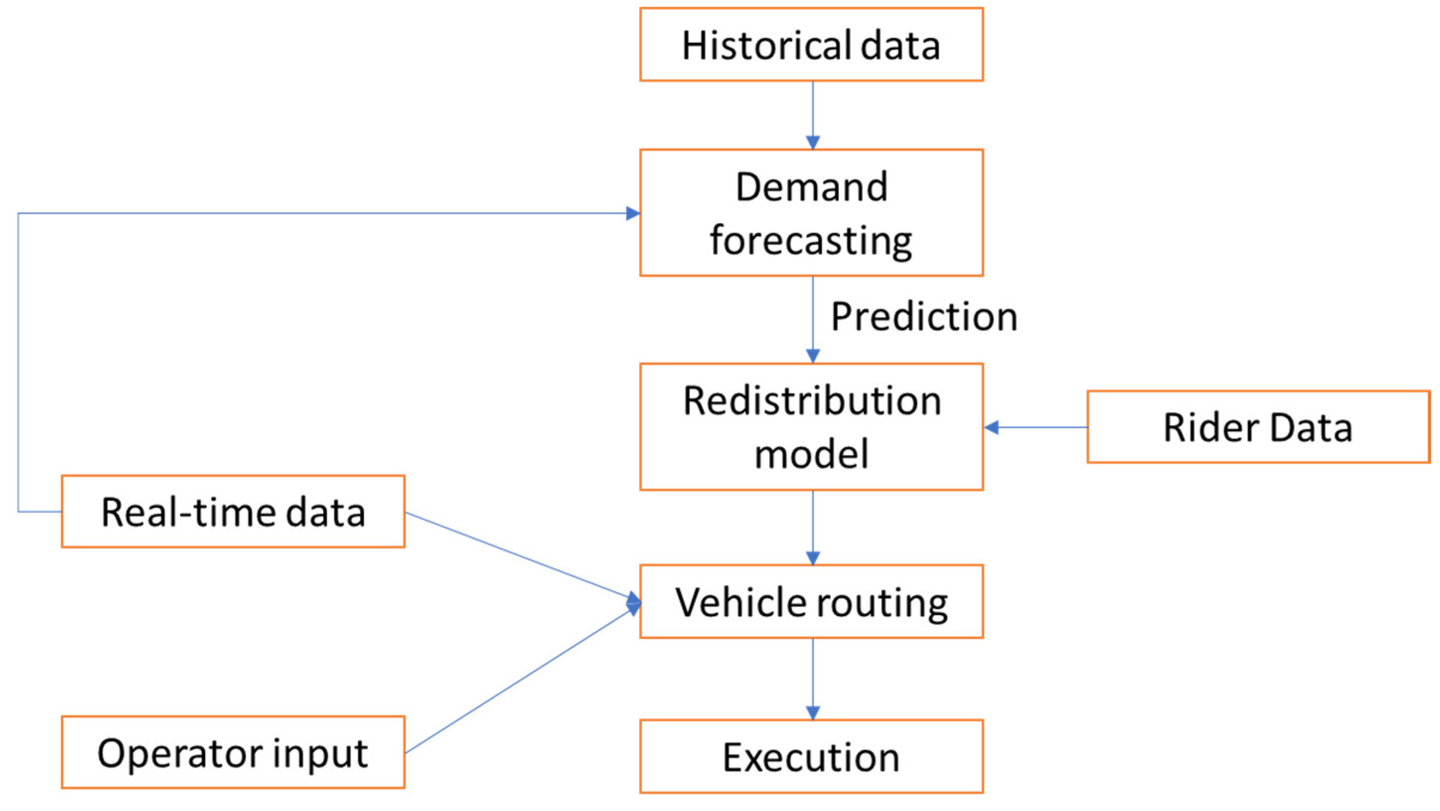
The Bureau of Transportation published a technical report in April 2016 that reported 3375 BSS stations distributed among 104 U.S. cities, though only 77% of those stations were connected to other scheduled public transportation systems [6]. These numbers demonstrate BSSs’ potential for reducing congestion. However, BSS rebalancing is a common recurring problem for many systems. Each day, an operator must visit all stations to redistribute (i.e., rebalance) bikes from full to empty stations to meet the projected daily demand. The bikes demand is reflected by the availability of bikes at each station in the BSS. Efficient BSS redistribution needs an accurate prediction of the bike count in a BSS. However, bike count prediction is challenging because the prediction models have to consider the variability of the demand patterns at the BSS stations. This variability is mainly because of the interaction between users and the BSS, as shown in Figure 1. Recently, many research papers have adopted machine learning and statistical models to solve the bike count prediction problem [7,8,9,10,11]. In this paper, we assume the demand is given and we know exactly the required number of bikes to drop off and pick-up at each station.
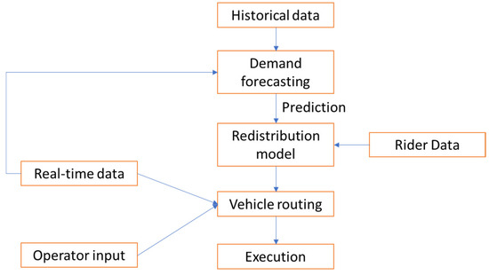
Figure 1.
Model interactions [12].
This redistribution problem is a generalized version of the traveling salesman problem (TSP), which involves determining the shortest route that visits all stations and returns to the original station. The TSP is an NP-hard problem where finding an exact optimal solution for large systems is currently impossible given limited time and computational resources (i.e., algorithms with exponential time complexity are guaranteed to find an exact solution).
In this paper, we propose a fast and accurate algorithm for solving the static bicycle rebalancing problem (SBRP) using multiple trucks. Our developed algorithm has three stages: network clustering, tour construction, and tour improvement. A set of approximate solutions are built in the first stage of the algorithm and are then improved using a local search in the second stage. In the third stage, a global search by means of black hole algorithm (BHA) is performed to provide more accurate solutions.
In the first stage, we use the BHA to divide the network into non-overlapping subnetworks, but overlapping at the depot only, such that each subnetwork is compact in size. In addition, each subnetwork should be as balanced as possible where the sum of the demand of the subnetwork is close to zero.
In the second stage, each subnetwork’s respective SBRP is constructed using two sets of disjointed players. After the first and second set of players construct their preferences for each other, the deferred acceptance algorithm is used to find stable assignments between them.
In the final step, the constructed tours are improved by performing a local search using the 2-opt algorithm. By limiting players’ preference lists, the proposed algorithm easily adapts to different sets of constraints. Accordingly, if demand predictions are known, the algorithm can solve dynamic rebalancing problems. Moreover, it is suitable for real-time applications where each subnetwork is solved independently, and both the local search algorithm and a matching algorithm can be executed in polynomial time.
This paper is organized as follows: The first and second sections present the introduction and the related work, respectively. In the third section, the methods used in this research are discussed. The problem statement is introduced in the fourth section. The proposed algorithm and the experimental work are presented in the fifth and sixth sections, respectively. Conclusions are drawn in the last section.
2. Related Work
Rebalancing BSS bike distribution is critical in guaranteeing customer satisfaction and system effectiveness [13,14]. Redistribution has been studied extensively in the literature and several efficient algorithms that maintain an equilibrium of bikes at each station have been proposed.
There are three types of rebalancing: static, dynamic, and incentivized. A fleet of trucks is typically used to redistribute bikes in static and dynamic rebalancing models. Static rebalancing, or SBRP, as it is commonly referred to in literature, is typically performed during periods of low demand, such as nighttime. This is because SBRP assumes the number of bikes needed at each station is constant or changes only slightly. In the dynamic bicycle repositioning problem (DBRP), the rebalancing outcome is affected because bike movement has a significant impact on bike demand at each station. It follows that demand predictions are necessary to solve DBRP. Incentivized rebalancing encourages users to participate in system rebalancing by suggesting slight changes to their planned journey through control signals, providing alternate routes that improve rebalancing, or even offering credits to return bikes to a station. In recent years, BSSs have evolved beyond the need for stations/docks, with users being able to deposit and pick up bikes anywhere within defined city boundaries. This type of bike-sharing, known as a free-floating bike-sharing system (FFBSS), offers benefits over standard BSSs, such as reduced bike theft and lower capital cost. Efficient rebalancing of this system is a crucial part of its success [15].
First proposed by Hernández-Pérez and Salazar-González [16], the problem is considered a one-commodity pick-up and delivery traveling salesman problem (1-PDTSP) and is known to be NP-hard. A good approach to problems of this complexity class is to use heuristic optimization techniques that determine a “good” near optimum tour (i.e., route).
These methods utilize stochastic search elements, which implement rules that guide the search towards favorable solutions. The aim is to converge on the optimum solution after many iterations. The solution obtained is not guaranteed to be the global optimum, and these types of solutions are therefore referred to as suboptimal.
Heuristic optimizations follow four common steps [17]: (i) choose an arbitrary initial solution, (ii) iteratively construct new and/or improved solutions using a mechanism/generation rule, (iii) evaluate the solutions using the objective function and report/retain the best among them, and (iv) once the stopping criterion is met, terminate the iterative search. Examples of heuristic algorithms include ant colony optimization (ACO), tabu search (TS), simulated annealing (SA), and genetic algorithms (GAs). These methods take inspiration from natural phenomena to solve NP-hard or NP-complete problems that have robustness or uncertainty issues, moderate or large sizes, or non-analytical optimization models.
Hernández-Pérez and Salazar-González solved the 1-PDTSP for instances of up to 75 locations using a branch-and-cut algorithm [16]. For solving larger instances (i.e., up to 500 locations) in a reasonable time, they proposed two heuristics: a greedy algorithm improved with the k-optimality criterion and a branch-and-cut procedure for finding an optimal local solution [18]. Shi et al. solved instances with 20–500 locations by utilizing a modified GA that incorporated a local search procedure instead of the mutation operation [19]. A scalable 1-PDTSP solution was proposed by Schuijbroek et al. [20]. Their approach used the maximum spanning star approximation to cluster stations. Furthermore, a cluster was assigned to each vehicle, and the redistribution tour was constructed to meet the required service level. Benchimol et al. [21] used integer programming to solve a variation of the SBRP and routing problem by allowing a single vehicle to visit the same location more than once. Li et al. [22] considered the multi-commodity (i.e., different bicycles) rebalancing problem and solved it using two-step logic. In the first step, the truck tour was constructed using a hybrid generic search. The pick-up/drop-off plan was then formulated using a greedy heuristic algorithm. Rainer-Harbach et al. [23] solved a multiple trucks with different capacities variation of the 1-PDTSP. In this variation, the start and end of the redistribution tours could not store bikes and were at separate locations. The problem was decomposed into two sub-problems: pick-up/drop-off planning and routing. Once vehicle routing schedules were constructed, the optimal pick-up/drop-off plan linked to that tour was determined through an integer programming model. An iterated tabu search heuristic was used by Ho and Szeto [24] to solve the SBRP. They made two assumptions in their formulation: (i) the truck could make multiple stops at the depot during rebalancing because the depot had sufficient bikes and capacity and (ii) the depot served as both the pick-up and drop-off node.
The DBRP was solved in real-time by Contardo et al. [25]. Their method utilized Benders decomposition and Dantzig–Wolfe techniques in conjunction with the most recent demand prior to repositioning decisions. The approach was not suitable when considering demand, which changes quickly. Shu et al. [26] predicted user demand over the entire horizon and attempted to find improved DBRP solutions by using a Poisson distribution. The DBRP was addressed by Ghosh et al. [27] who considered changing daytime demands. The problem was decomposed into two subproblems—vehicle routing and bike repositioning—through the use of abstraction mechanisms and Lagrangian dual decomposition. Zhang et al. considered a multi-truck, multi-commodity DBRP as a time–space network flow model. The resulting non-linear objective function was transformed into an equivalent mixed-integer programming model, which minimized the total unmet demand and route. This was solved with a novel heuristic for 200 stations and 5 vehicles in 47.12 s [28]. Wang and Szeto extended the SBRP by considering a green approach, which minimized the total CO2 emissions from repositioning vehicles in a mixed-integer linear programming model [29]. Shui and Szeto improved on this by considering the dynamic variant. This model minimized the total unmet demand and fuel and CO2 emission cost by using a rolling horizon approach and an enhanced artificial bee colony algorithm [30].
Pal and Zhang considered the FFBSS problem by solving a large scale static complete rebalancing problem (SCRP) that allowed the same vehicle to make multiple visits to a node. A variable neighborhood descent algorithm was used with a hybrid nested large neighborhood search to solve an SCRP with 3000 bikes, 450 stations, and 30 vehicles in a mean total time of approximately 4.2 h [15]. Du et al. proposed an integer linear programming model to optimize an FFBSS with malfunctioning bike collection. A greedy genetic heuristic was used to solve an instance with 450 stations, 1000 functioning and 100 malfunctioning bikes, and 13 trucks in a mean solve time of 4.2 h [31]. The dynamic case has seen significantly less attention. Caggiani et al. proposed a framework for dealing with dynamic FFBSSs by performing spatio-temporal clustering on historical data, followed by a non-linear autoregressive neural network to predict demand. This was input into a spatio-temporal microsimulation, which determined optimal repositioning flows and bike distribution patterns. [32]. Ruijing et al. considered the incentivized FFBSS rebalancing model. A stochastic simulation optimization model, which adopted a rank and search methodology, was used to maintain expected satisfactory service levels while maximizing total expected daily profit. Their findings suggested that an optimal incentive-based rebalancing plan could achieve higher bike utilization [33].
3. Methods
This section introduces the modeling techniques used in this paper.
3.1. Black Hole Algorithm (BHA)
The black hole algorithm (BHA) is a black hole-inspired metaheuristic algorithm [34,35]. The algorithm begins by randomly choosing many solutions within the search space. The objective function is used to evaluate these solutions; the optimal solution is labeled the “black hole” and all others are labeled “stars”. During each iteration, stars are moved toward the black hole and each new star’s cost is reevaluated. The solution is improved on if a star’s cost is better than the black hole’s. When this happens, the star becomes the new black hole, and the old black hole becomes a star. Stars are removed from the population of solutions and are subsequently replaced by a randomly generated star if they become close to the black hole. This process continues to iterate until the stopping criterion is met.
3.2. Deferred Acceptance Algorithm (DAA)
Introduced by Gale and Shapley [36], the deferred acceptance algorithm finds a stable assignment for two equal sets of size N, one consisting of men and the other women, each of whom has an ordered list of their preferred partners to marry from the opposite sex. A stable assignment is formed when there is no incentive for any couple to leave their assigned mate for another. The algorithm has an average complexity and worst case of and , respectively [37,38]. During the first stage, men propose to the first woman on their preference list. Each woman accepts the best proposal on her preference list, rejecting all others. These proposals are said to be in a state of deferred acceptance. In the second stage, each man previously rejected proposes to their second preference. Each woman then accepts the better of their deferred acceptance state offers and best proposal during the current stage, rejecting all other offers. Men continue proposing until each man holds a deferred proposal, at which point each woman accepts the proposal they currently hold, and the algorithm terminates.
3.3. The 2-Opt Local Search Algorithm
The 2-opt algorithm is a tour-improving algorithm which iteratively improves a solution once one is established by the deferred acceptance algorithm. It follows that the 2-opt solution quality depends on the deferred acceptance algorithm’s initial solution. The 2-opt algorithm has a complexity of . The algorithm consists of three stages: (i) perform a local search via removal of two edges from the solution; (ii) reconnect the two created paths to form a new, valid solution; and (iii) replace the original solution if the new solution minimizes the objective function. These three steps are repeated until no improvements can be made.
4. Problem Statement for a Subnetwork
Before starting the problem, we define the term “NotSpot”, adopted from [39], as a bike station patrons who want to return or pick up a bike considered unusable because the station is full or empty. Similarly, a bike station is considered a NotSpot if there are more or less than a certain threshold of bikes. We define these thresholds as and . In addition, while beyond the scope of the paper, it should be noted that historical data for a given station can be used to estimate the and thresholds for that station.
Given a fully connected network , where is the set of NotSpots in the bike system, including the depot, and is the set of all links connecting the vertices in the network, we partition this network into subnetworks (i.e., g1 = (v1, e1) … gp = (vp, ep)), where is also the number of trucks. Because we assume there is only one depot, all subnetworks overlap only at the depot.
To each node in each subnetwork, we assign an integer , which represents the number of needed/pick-up bikes. If is negative, then bikes are removed from a NotSpot. Consequently, station becomes a pick-up station. If is positive, then bikes need to be dropped at a NotSpot, and station becomes a drop-off station. The cost is assigned for the link between i and j.
In this paper, the adapted heuristics aim to generate a good/suboptimal truck tour that rebalances the NotSpot stations. The input data consists of a list of NotSpots and the depot, the distances matrix of each subnetwork, and the demand of the NotSpots. Each subnetwork will be served by only one truck with a maximum capacity .
The tour is considered optimum by minimizing the total traveling distances () and total residuals ( as follows in Equation (1):
where
, and are the residuals at NotSpot , the maximum capacity of the truck, and the available bike spots on the truck before serving NotSpot , respectively. This is performed for each subgraph (). These constraints guarantee no empty or full trucks will arrive at pick-up and drop-off NotSpot stations, respectively. A complete formulation of the problem can be found in [40].
This problem is 1-PDTSP because we assume that only one type of bike is present in the BSS and that the tour starts and ends at the depot. Furthermore, the truck begins the tour below or at maximum bike carrying capacity. However, in the experimental work, we assumed that the truck always leaves the depot empty.
5. The Proposed Algorithm
The proposed algorithm has three stages. The first stage is the network clustering. In this phase, the BHA is used to divide the whole network into subnetworks, overlapping at the depot only, such that the subnetworks are compact and as balanced as possible. The second phase, the most important phase, is the tour construction. In this stage, we construct the tour for each subnetwork independently. The tour construction is modeled as a cooperative game and then we recursively apply the deferred acceptance algorithm times, where M is the number of NotSpots in the subnetwork, to match two disjoint sets: the NotSpot stations and the partial tours. Matching is performed to ensure that, post-construction phase, each tour contains all NotSpot stations, with each NotSpot station appearing once in the tour. The 2-opt algorithm improves the constructed tours in the final phase, and the best tour is selected as the problem’s solution. Following, we will describe the details of the network clustering, tour construction, and improvement.
5.1. Network Clustering Using the BHA
In this stage, we use the BHA to divide the whole network into a set of subnetworks {, where and for . The number of subnetworks equals the number of trucks. In addition, all subnetworks have almost equal sizes. The cost of each subnetwork is computed using Equation (2):
where
- C
- constant ;
- is the distance from the depot to the first NotSpot in the sub-vector;
- is the distance from the last NotSpot in the sub-vector to the depot.
We start by randomly creating many station sequences. Each sequence is simply a vector of random permutation of all NotSpots. We evaluate each sequence by dividing the vector of randomly permuted NotSpots into contiguous sub-vectors where the length of each sub-vector equals the size of the corresponding subnetwork. The BHA assigns all but the lowest cost sequence as stars, with the lowest cost sequence being assigned the black hole role. Each star is then subject to the following:
- Calculate the distance between the star and the black hole using , where is the indicator function,
- , and and are the station IDs at the position in the black hole solution (vector/sequence) and star solution (vector/sequence), respectively.
- Replace the star with a randomly generated star if .
- Identify the set of positions on star tour such that , where .
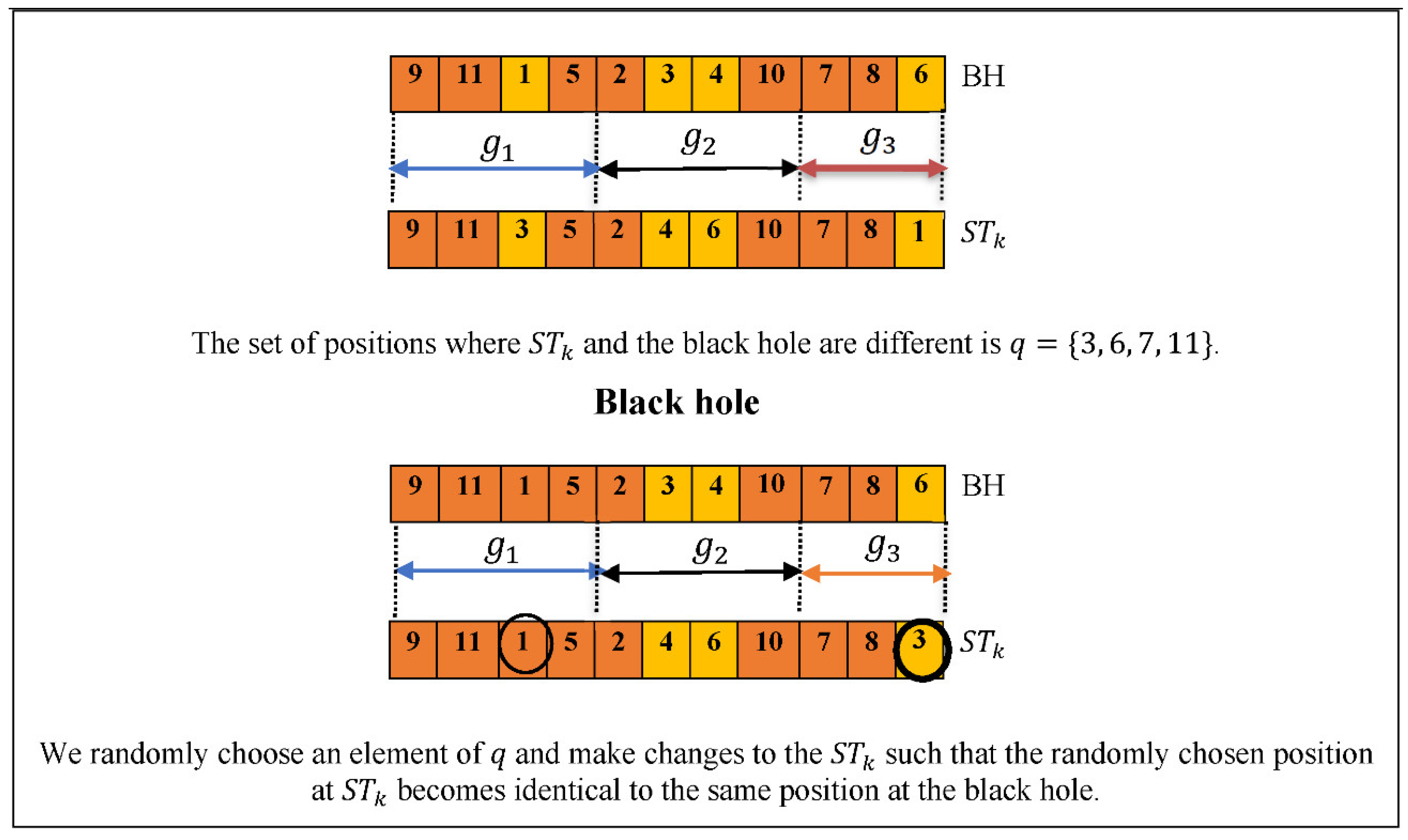
- Randomly choose one element of the set and change , as shown in Figure 2.
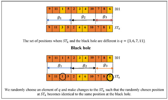 Figure 2. Illustration of the modification of the solution to converge towards the black hole solution.
Figure 2 shows an illustration of BHA’s modification process. In this example, the network consists of 11 NotSpots and we want to divide it into three subnetworks of size 4, 4, and 3, respectively. At the start of the modification, the best solution is the black hole, which groups nodes {9, 11, 1, 5}, nodes {2, 3, 4, 10}, and nodes {7, 8, 6} as three non-overlapping subnetworks. The example shows that when comparing the black hole and a star , four locations on are found that are different from the black hole. Subsequently, one of these four locations is randomly chosen by the BHA to be made identical to the black hole’s location, while ensuring the modified contains only one location for each NotSpot.
Following the application of the four BHA steps to each star, costs are considered, and the lowest cost black hole is chosen for the next iteration. This continues until the stopping criterion is satisfied.
5.2. Tour Construction Using the Deferred Acceptance Algorithm
The tour construction phase works on each subnetwork independently. The proposed algorithm has the goal of constructing good tours, where is the number of NotSpots in the subnetwork . Each tour is considered a Hamiltonian path that consists of a depot and M NotSpots.
The tour construction is considered a cooperative game between two disjointed sets of players. One player’s set comprises partial tours. Each of these tours is characterized by the current load for the truck once the last NotSpot in the partial tour has been served. Each partial tour has the goal of finding the next NotSpot i to serve. Consequently, the cost function, shown in Equation (3), is used to build an ascending list for each partial tour.
where is a constant between 0.1 and 1.0, is defined previously as the maximum truck capacity, is the number of available bikes on the truck after serving NotSpot , is a constant , and is the distance in meters between the last station in the partial tour and NotSpot . The partial tour’s preference list order is such that the preferred NotSpot has the smallest value of Equation (2). Furthermore, it only contains NotSpots NOT shown in its current path.
The second player’s set contains NotSpots. Preference lists for each NotSpot i are constructed to include only partial tours that do not yet contain i. The partial tours’ preference list is ordered so that the first and last preferences are the tours that minimize and maximize the residual at NotSpot i, respectively. That is, the top tour in this player’s list is the best at achieving station demand (has the lowest absolute residual) and the last tour is the worst (has the highest absolute residual).
After building preference lists for each player, the deferred acceptance algorithm is used to find a stable assignment between the partial tours and the NotSpots. Following this, each partial trip has its matched NotSpot stacked on its end, and the current number of bikes in the truck is updated.
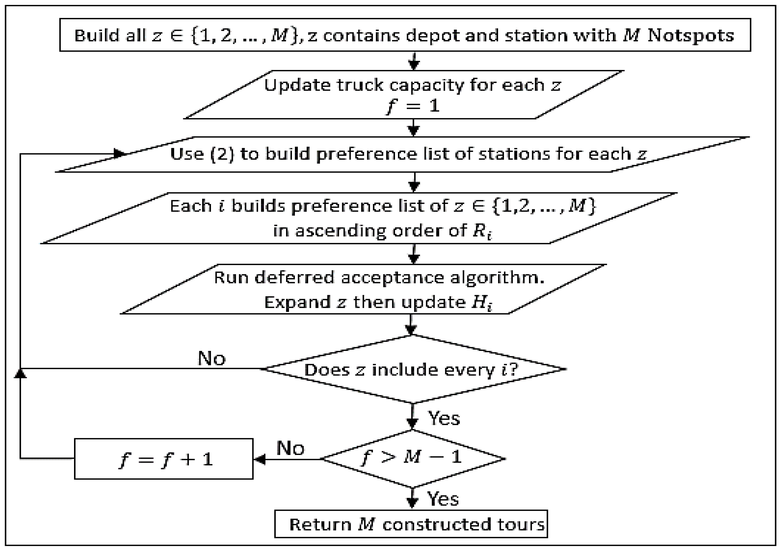
Lastly, the partial trip is inspected for the number of NotSpots it contains. ALL NotSpots must be included, otherwise the preference list for each player is reconstructed and another game is played. The algorithm is terminated if all NotSpots ARE included. A flowchart of the proposed algorithm can be seen below in Figure 3.
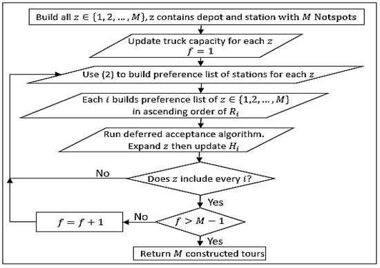
Figure 3.
Flowchart of the deferred acceptance algorithm.
5.3. Tour Construction Example
We consider a fully connected undirected graph containing a depot and three NotSpot stations for the purpose of illustrating the tour construction algorithm. We assume a square is formed from the vertices, the sides of which are 1000 m long, where the link between and has a length of 1200 m, as shown in Figure 4. We set Q, , and as 10, 0.5, and 0.002, respectively. Furthermore, we assume the truck leaves the depot with four bikes.
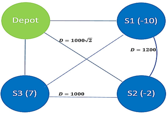
Figure 4.
Example graph (number in parentheses is the NotSpot demand).
The following steps are taken to construct the tour algorithm:
- Build S1, S2, S3, such that each contains a depot and one of the three NotSpot stations. Update for each tour, as shown in Equation (4).
- Use Equation (3) to determine the preference list for each . Set to 0.5. This gives preference to stations which reduce the truck capacity to half.
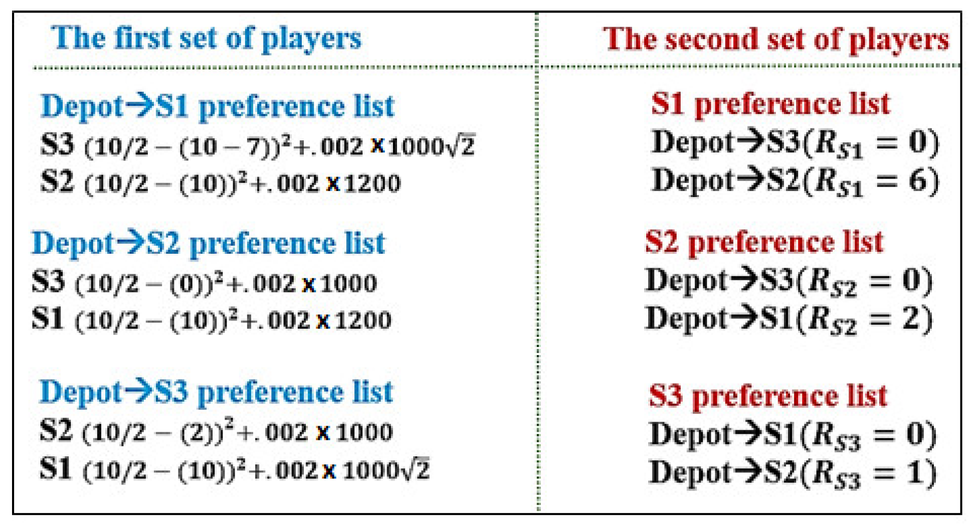
- Build preference lists for each such that the which minimizes is the first preference. See Figure 5.
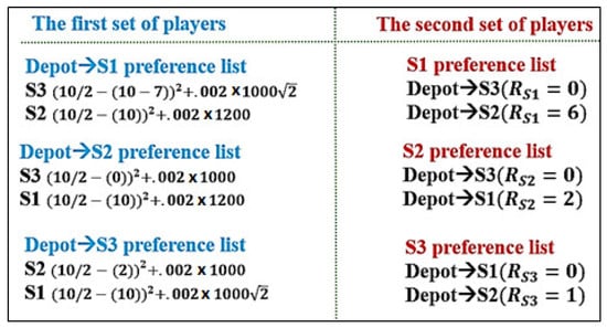 Figure 5. The preference list for the two sets of players.
 - Using the deferred acceptance algorithm, match with . Given the result, each is expanded. This can be seen in Equation (5) and Figure 6.
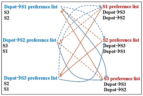 Figure 6. Illustration of the matching: when offers are made by the partial tours, the first and second partial tours select S3, with the third selecting S2. The first partial tour is accepted by S3 (S3′s first choice), and the third partial tour is accepted by S2. The second partial tour makes an offer to S1 in the second stage. S1 accepts and the game results in a stable match.
 - Update then expand each .
- Ensure each is included in ; go to step 2 if there are less than 3 stations.
5.4. Tour Improvement Using 2-Opt Local Search Algorithm
After tour construction, there exist different tours, each of which contains NotSpots. The cost of every M constructed tour is evaluated during tour improvement using Equation (6).
where is the length of link in meters, is the residual at NotSpot , and is the same constant used in Equation (2).
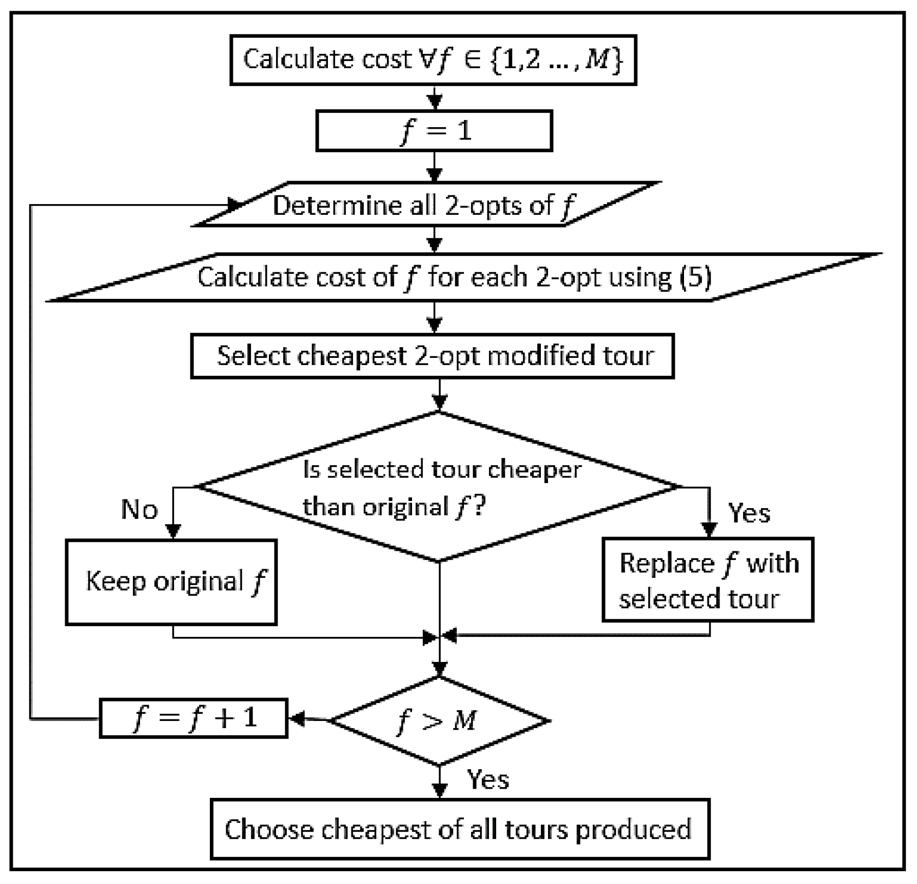
For each constructed tour, the 2-opt algorithm is run, and we evaluate the cost of each new tour, selecting the one that lowers the cost function. At the end of this phase, we select the tour with the lowest cost out of the tours. A flowchart of the proposed algorithm can be seen below in Figure 7.
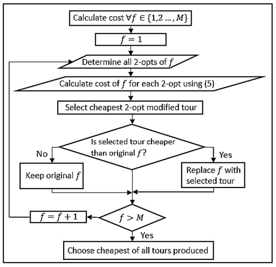
Figure 7.
Flowchart of the 2-opt local search algorithm.
If we assume that, then an edge on the path of the truck can be represented using the Equation (7)
where is the matrix representing the distance between the different vertices and is an integer that takes the value of 1 if the edge between and is considered and 0 otherwise. For each subnetwork, the 2-opt local search algorithm attempts to solve the following problem formulation:
Subject to:
where represents the index of the current station served in the path, represents the number of bikes in the truck before serving station , and is the number of available bike spots on the truck before serving NotSpot .
6. Experimental Work
This section is divided into three subsections. In the first subsection, we use simulation data to test our proposed algorithm. In the second subsection, we choose several medium-sized benchmark instances that have known solutions. Then we solve these instances using our algorithm and compare the result to the best-known solutions from the literature. Finally, in the third subsection, we solve large benchmark instances, which vary in size from 150 to 564 nodes. The solutions to the different problems presented in this paper were performed using an OptiPlex 9020 Dell desktop, which has 8 GB RAM and an Intel® Core™ i7-4790 CPU @ 3.60 GHz. MATLAB 2015b was used to code the proposed algorithm. The proposed algorithm has the advantage of only having two hyperparameters: and . We set C equal to 0.02 and varied from 0.1 to 1.0.
6.1. Simulation Data
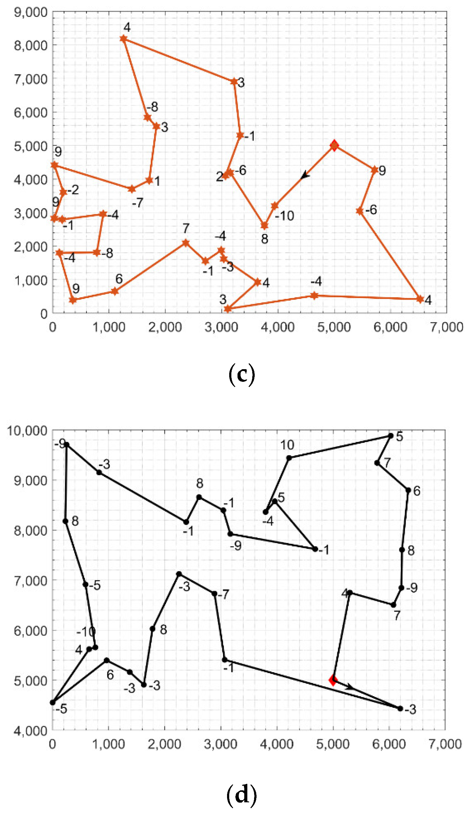
We created a set of random instances to evaluate the proposed algorithm’s performance. We randomly generated five instances, each consisting of 90 vertices. The vertices were randomly spread out in a square area equal to 10,000 by 10,000 m. The depot was located at the center of the square. The demand of each station was randomly drawn from the set . We solved the rebalancing problem for each instance at a different . We assumed there were three equal capacity trucks and that they started empty at the depot. Because of the randomness in the first stage of the algorithm, we ran the algorithm 20 times for each instance and for each . Table 1 shows the value of the demand imbalance, the vehicle capacity, the mean and standard deviation of running time in seconds, the mean and standard deviation of the total distance traveled by the trucks to rebalance the whole network, and the median and median absolute deviation of the whole network absolute residual. As shown in Table 1, the first and fourth simulated instances had an imbalance of 32 and 35, respectively, where a positive value means that the network needs bikes and a negative value means that the network has surplus bikes. In both networks, the proposed algorithm found the routes that minimized the residual as much as possible in less than 3 min. The other three networks had negative demand/pick-up bikes. For example, the last network had 65 extra bikes. Our algorithm found solutions for Q equals 30 and 20 in less than 3 min. Moreover, absolute residuals were very small. It is worth noting that the solution for this network using Q = 10 has 35 residual bikes. This is because the network has 65 extra bikes and the total capacity of the three trucks is 30 bikes. In other words, the trucks completed their tours and returned to the depot fully loaded with 10 bikes each. Figure 8 shows one of the solutions for the first instance. The top panel shows the three tours (Figure 8a) and the bottom panels show each truck tour separately (Figure 8b–d). There was a significant overlap between the three tours because the whole network is divided based on an objective function in the distance and demand.

Table 1.
The evaluation of the proposed algorithm using five randomly generated instances.
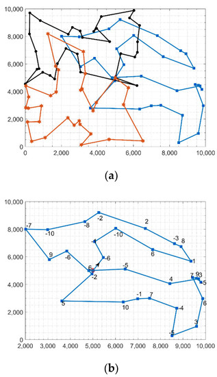
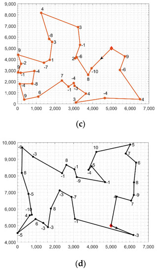
Figure 8.
A solution for the first randomly generated instance. Panel (a) shows the three established routes for the trucks. Panels (b–d) show the constructed routes for each truck in addition to the demand.
6.2. Medium-Sized Benchmark Instances
The algorithm was tested on real medium-sized instances with adequate (i.e., not close to zero) demand. Instances were gathered from Ciudad de Mexico, Mexico; Dublin, Ireland; Minneapolis, United States; and Denver, United States, which had total respective demands of −87, −64, −87, and −35. We assumed that the number of subnetworks was given by the BSS operator and depends on the number of available trucks. Moreover, we chose almost equal-sized subnetworks. In this experimental work, we divided Dublin, Denver, Ciudad de Mexico, and Minneapolis into two, two, three, and four subnetworks, respectively. Recall that the first stage is not deterministic, and each run of the algorithm returns a different clustering of the whole network. We ran the algorithm 20 times and found the 20 solutions for each instance. Table 2 shows the best-known solution in the literature for the four instances along with the summary statistics of the running time, distance, and absolute bike residuals of the proposed algorithm. In general, the distance of the proposed algorithm is larger than the best-known solutions for large . However, for small , the proposed algorithm is better. Note also that the mean running times for the largest instance in this table are 143.6, 130.32, and 51.85 s for = 30, 20, and 10, respectively, which makes the proposed algorithm a real-time rebalancing algorithm.

Table 2.
The evaluation of the proposed algorithm using medium-size benchmark instances.
In terms of absolute bike residuals, we highlight that the residual in the table is a result of an imbalance in the total demand. In the Denver instance, for example, the total demand is −35. This means there were 35 more pick-up bikes than drop-off bikes. For this instance, rebalancing with two trucks—each of which had a 10-bike maximum capacity and was carrying 10 bikes at the end of the tour—yields a best solution with a residual of 15 bikes.
6.3. Large-Size Benchmark Instances
We tested the proposed algorithm using benchmark instances that varied in size, from 150 to 564 stations. The main goal of this subsection is to show the ability of the proposed algorithm to solve large instances in short computational times and hence its suitability for real-time applications. Recall that the running time reported above is the clustering time (first stage) plus the summation of the time needed to solve each subnetwork independently. Consequently, significant further improvements in computational times can be achieved by parallelizing the individual subnetwork route improvements by a factor of at least 1.5. Table 3 (following the Conclusions) shows the worst running time to be 1 h and is taken by the Bruxelles instance at = 30. This is the time needed if we sequentially solve the problem, meaning we perform for a cluster and then solve for each cluster in order. One advantage of the proposed algorithm is that we can perform the clustering and then solve for the subnetworks in parallel. If we compute the clustering time and the time needed to solve each subnetwork of the Bruxelles instance at = 30, we find that the clustering time for this example is 488.56 s and the maximum time taken to solve one subnetwork is 598.38 s. This means that if we performed the clustering and then solved the different subnetworks independently (i.e., in parallel) using different cores, the running time drops by almost 30% of the sequential running time. This makes the proposed algorithm suitable for real-time applications and dynamic rebalancing. Currently, the use of a sequential algorithm produces solutions in a computational time that is 37% less than that of the best heuristics available in the literature. As mentioned, this can be increased by a factor of 1.5 if the code is run in parallel, given the fact that each sub-tour is optimized independently. It should be noted that the gap between the proposed algorithm and the best solutions are 69%, on average, for these large instances. However, further improvements, which are beyond the scope of this paper, are being made to the algorithm to reduce this gap.

Table 3.
The comparison of the proposed algorithm and BHA based heuristic using large-size benchmark instances.
6.4. Comparison with Another Heuristic
For the sake of completeness, we compare the prosed algorithm with the BHA based heuristic. We used the black hole to partition the whole network as explained in subsec 5.1 (i.e., Network Clustering Using the BHA). Then, for each subnetwork we use BHA to minimize the total traveling distances () and total residuals ( and hence find a good solution to rebalance subnetwork . We should highlight that the BHA allows stars/solutions where an empty or full truck arrives at a pick-up and drop-off NotSpot. The BHA assigns an infinity cost to such a star, keeps it in the solutions population, and processes it as a regular star in the hope it may yield a good solution. As shown in the comparison results in Table 4, for some instances the BHA based heuristic failed to find a Hamiltonian path where the truck at least partially satisfies the demand of every NotSpot. Moreover, our proposed algorithm yielded a better solution for most of the big instances.

Table 4.
The evaluation of the proposed algorithm using large-size benchmark instances.
7. Conclusions
This study proposed a real-time heuristic algorithm for the static rebalancing of a BSS. The proposed algorithm has three stages. The first stage is based on the BHA, where the BSS network is divided into subnetworks overlapping at the depot only. In the second stage, we modeled the rebalancing of each subnetwork as a cooperative game, and the deferred acceptance algorithm was used to construct a good initial solution for each subnetwork independently. In the third stage of the algorithm, the initial solutions for each subnetwork were improved using the 2-opt algorithm.
The proposed algorithm was tested using randomly generated instances, each consisting of 90 stations. When we divided the network into three subnetworks, we solved the rebalancing problem in less than 3 min. Moreover, the algorithm was used to solve medium-sized real benchmark instances with sizes varying from 45 to 116 stations. We compared the quality of our solution to the best-known solutions for these instances. Based on this comparison, we concluded that at = 30 or 20, we obtained lower quality solutions but solved the problem in less than 3 min. For small , we found the solution in less than 2 min, and the tours were better than the best-known solutions in terms of distance.
We also solved large benchmark instances whose sizes varied from 150 to 565 stations. A good solution was found in approximately 1 h. Furthermore, we compared the proposed algorithm solution of large benchmark instances with the solutions obtained using BHA based heuristic and the best-known solutions. The comparison showed a promising performance of the proposed algorithm. We should highlight that the advantage of our solution is that modeling the rebalancing problem as a game and allowing each player to have his own preference list will enable us to solve the problem even if each player has his own objective function Finally, we demonstrated that the proposed algorithm could be enhanced further by parallelizing the solution process of the subnetworks. In the future, we will examine ways to improve solution quality while also generalizing to large instances and addressing more complex constraints such as time BBS with time windows.
Author Contributions
Conceptualization, M.E., Y.B. and H.A.R.; methodology, M.E., Y.B., H.A.R. and M.M.; software, M.E., M.M. and A.S.; validation, M.E., Y.B., H.A.R. and M.M.; formal analysis, M.E. and Y.B.; investigation, M.E., M.M. and S.G.; resources, M.M. and S.G.; data curation, A.S.; writing—original draft preparation, M.E., J.P. and A.S.; writing—review and editing, A.S., J.P. and M.M.; visualization, A.S.; supervision, H.A.R. and S.G.; project administration, J.P. and A.S.; funding acquisition, H.A.R. All authors have read and agreed to the published version of the manuscript.
Funding
This effort was funded by the U.S. Department of Transportation award 69A3551747123 as part of the University Mobility and Equity Center. Also, This research was partially supported by the Motor Accident Insurance Commission (MAIC) Queensland.
Institutional Review Board Statement
Not applicable.
Informed Consent Statement
Not applicable.
Data Availability Statement
The instances used in this paper are available at https://github.com/mohammed-QUT/A-Feasible-Solution-for-Rebalancing-Large-Scale-Bike-Sharing-Systems.git.
Conflicts of Interest
The authors declare no conflict of interest.
References
- Schrank, D.; Lomax, T.; Eisele, B. 2012 Urban Mobility Report. Available online: https://static.tti.tamu.edu/tti.tamu.edu/documents/umr/archive/mobility-report-2012.pdf (accessed on 29 November 2021).
- Schrank, D.L.; Lomax, T.J. 2009 Urban Mobility Report; Texas Transportation Institute, Texas A&M University: College Station, TX, USA, 2009. [Google Scholar]
- Arnott, R.; Small, K.J.A. The economics of traffic congestion. Am. Sci. 1994, 82, 446–455. [Google Scholar]
- Shaheen, S.A.; Guzman, S.; Zhang, H. Bikesharing in Europe, the Americas, and Asia: Past, present, and future. Transp. Res. Rec. 2010, 2143, 159–167. [Google Scholar] [CrossRef] [Green Version]
- Almannaa, M.H.; Elhenawy, M.; Masoud, M.; Rakha, H.A. A New Mathematical Approach to Solve Bike Share System Station Imbalances Based On Portable Stations. In Proceedings of the 2019 IEEE Intelligent Transportation Systems Conference (ITSC), Auckland, New Zealand, 27–30 October 2019; IEEE: Manhattan, NY, USA, 2019; pp. 1721–1726. [Google Scholar]
- Hu, W. Times TNY, Editor 2020. Available online: https://www.nytimes.com/2020/03/14/nyregion/coronavirus-nyc-bike-commute.html (accessed on 29 November 2021).
- Firestine, T. Bike-Share Stations in the U.S. Technical Report. 2016. Available online: https://www.bts.gov/sites/bts.dot.gov/files/legacy/Bike-Share%20Data_1.PDF (accessed on 29 November 2021).
- Ashqar, H.I.; Elhenawy, M.; Almannaa, M.H.; Ghanem, A.; Rakha, H.A.; House, L. Modeling bike availability in a bike-sharing system using machine learning. In Proceedings of the 2017 5th IEEE International Conference on Models and Technologies for Intelligent Transportation Systems (MT-ITS), Naples, Italy, 26–28 June 2017; pp. 374–378. [Google Scholar]
- Ashqar, H.I.; Elhenawy, M.; Rakha, H.A. Modeling bike counts in a bike-sharing system considering the effect of weather conditions. Case Stud. Transp. Policy 2019, 7, 261–268. [Google Scholar] [CrossRef]
- Almannaa, M.H.; Elhenawy, M.; Rakha, H.A. Dynamic linear models to predict bike availability in a bike sharing system. Int. J. Sustain. Transp. 2020, 14, 232–242. [Google Scholar] [CrossRef]
- Ashqar, H.I.; Elhenawy, M.; Rakha, H.A.; Almannaa, M.; House, L. Network and station-level bike-sharing system prediction: A San Francisco bay area case study. J. Intell. Transp. Syst. 2021, 1–11. [Google Scholar] [CrossRef]
- Regue, R.; Recker, W. Proactive vehicle routing with inferred demand to solve the bikesharing rebalancing problem. Transp. Res. Part E Logist. Transp. Rev. 2014, 72, 192–209. [Google Scholar] [CrossRef]
- Fricker, C.; Gast, N. Incentives and redistribution in homogeneous bike-sharing systems with stations of finite capacity. Eur. J. Transp. Logist. 2016, 5, 261–291. [Google Scholar] [CrossRef] [Green Version]
- Chemla, D.; Meunier, F.; Wolfler Calvo, R. Bike sharing systems: Solving the static rebalancing problem. Discret. Optim. 2013, 10, 120–146. [Google Scholar] [CrossRef]
- Pal, A.; Zhang, Y. Free-floating bike sharing: Solving real-life large-scale static rebalancing problems. Transp. Res. Part C Emerg. Technol. 2017, 80, 92–116. [Google Scholar] [CrossRef]
- Hernández-Pérez, H.; Salazar-González, J.J. A branch-and-cut algorithm for a traveling salesman problem with pickup and delivery. Discret. Appl. Math. 2004, 145, 126–139. [Google Scholar] [CrossRef] [Green Version]
- Lee, K.Y.; El-Sharkawi, M.A. Modern Heuristic Optimization Techniques: Theory and Applications to Power Systems; John Wiley & Sons: Hoboken, NJ, USA, 2008; Volume 39. [Google Scholar]
- Hernández-Pérez, H.; Salazar-González, J.J. Heuristics for the one-commodity pickup-and-delivery traveling salesman problem. Transp. Sci. 2004, 38, 245–255. [Google Scholar] [CrossRef]
- Shi, X.; Zhao, F.; Gong, Y. Genetic algorithm for the one-commodity pickup-and-delivery vehicle routing problem. In Proceedings of the 2009 IEEE International Conference on Intelligent Computing and Intelligent Systems, Shanghai, China, 20–22 November 2009; IEEE: Manhattan, NY, USA, 2009; pp. 175–179. [Google Scholar]
- Schuijbroek, J.; Hampshire, R.C.; Van Hoeve, W.J. Inventory rebalancing and vehicle routing in bike sharing systems. Eur. J. Oper. Res. 2017, 257, 992–1004. [Google Scholar] [CrossRef] [Green Version]
- Benchimol, M.; Benchimol, P.; Chappert, B.; De La Taille, A.; Laroche, F.; Meunier, F.; Robinet, L. the stations of a self service “bike hire” system. RAIRO-Oper. Res. 2011, 45, 37–61. [Google Scholar] [CrossRef]
- Li, Y.; Szeto, W.; Long, J.; Shui, C.S. A multiple type bike repositioning problem. Transp. Res. Part B Methodol. 2016, 90, 263–278. [Google Scholar] [CrossRef] [Green Version]
- Rainer-Harbach, M.; Papazek, P.; Hu, B.; Raidl, G.R. Balancing bicycle sharing systems: A variable neighborhood search approach. In Proceedings of the European Conference on Evolutionary Computation in Combinatorial Optimization, Vienna, Austria, 3–5 April 2013; Springer: Berlin/Heidelberg, Germany, 2013; pp. 121–132. [Google Scholar]
- Ho, S.C.; Szeto, W.Y. Solving a static repositioning problem in bike-sharing systems using iterated tabu search. Transp. Res. Part E Logist. Transp. Rev. 2014, 69, 180–198. [Google Scholar] [CrossRef] [Green Version]
- Contardo, C.; Morency, C.; Rousseau, L.-M. Balancing a Dynamic Public Bike-Sharing System; Cirrelt: Montreal, QC, Canada, 2012; Volume 4. [Google Scholar]
- Shu, J.; Chou, M.C.; Liu, Q.; Teo, C.-P.; Wang, I.-L. Models for effective deployment and redistribution of bicycles within public bicycle-sharing systems. Oper. Res. 2013, 61, 1346–1359. [Google Scholar] [CrossRef]
- Ghosh, S.; Varakantham, P.; Adulyasak, Y.; Jaillet, P. Dynamic repositioning to reduce lost demand in bike sharing systems. J. Artif. Intell. Res. 2017, 58, 387–430. [Google Scholar] [CrossRef]
- Zhang, D.; Yu, C.; Desai, J.; Lau, H.; Srivathsan, S. A time-space network flow approach to dynamic repositioning in bicycle sharing systems. Transp. Res. Part B Methodol. 2017, 103, 188–207. [Google Scholar] [CrossRef]
- Wang, Y.; Szeto, W.Y. Static green repositioning in bike sharing systems with broken bikes. Transp. Res. Part D Transp. Environ. 2018, 65, 438–457. [Google Scholar] [CrossRef]
- Shui, C.S.; Szeto, W.Y. Dynamic green bike repositioning problem–A hybrid rolling horizon artificial bee colony algorithm approach. Transp. Res. Part D Transp. Environ. 2018, 60, 119–136. [Google Scholar] [CrossRef] [Green Version]
- Du, M.; Cheng, L.; Li, X.; Tang, F. Static rebalancing optimization with considering the collection of malfunctioning bikes in free-floating bike sharing system. Transp. Res. Part E Logist. Transp. Rev. 2020, 141, 102012. [Google Scholar] [CrossRef]
- Caggiani, L.; Camporeale, R.; Ottomanelli, M.; Szeto, W.Y. A modeling framework for the dynamic management of free-floating bike-sharing systems. Transp. Res. Part C Emerg. Technol. 2018, 87, 159–182. [Google Scholar] [CrossRef]
- Wu, R.; Liu, S.; Shi, Z. Customer incentive rebalancing plan in free-float bike-sharing system with limited information. Sustainability 2019, 11, 3088. [Google Scholar] [CrossRef] [Green Version]
- Hatamlou, A. Black hole: A new heuristic optimization approach for data clustering. Inf. Sci. 2013, 222, 175–184. [Google Scholar] [CrossRef]
- Zhang, J.; Liu, K.; Tan, Y.; He, X. Random black hole particle swarm optimization and its application. In Proceedings of the 2008 IEEE International Conference Neural Networks and Signal Processing, Nanjing, China, 7–11 June 2008; pp. 359–365. [Google Scholar]
- Gale, D.; Shapley, L.S. College admissions and the stability of marriage. Am. Math. Mon. 2013, 120, 386–391. [Google Scholar] [CrossRef] [Green Version]
- Ng, C.; Hirschberg, D.S. Lower bounds for the stable marriage problem and its variants. SIAM J. Comput. 1990, 19, 71–77. [Google Scholar] [CrossRef]
- Wilson, L.B. An analysis of the stable marriage assignment algorithm. BIT Numer. Math. 1972, 12, 569–575. [Google Scholar] [CrossRef]
- Goodyear, S. Mapping the Imbalances of New York’s Popular, Troubled Bike-Share. Available online: http://www.citylab.com/commute/2014/03/mapping-imbalances-new-yorks-popular-troubled-bike-share/8699/ (accessed on 29 November 2021).
- Dell’Amico, M.; Hadjicostantinou, E.; Iori, M.; Novellani, S.J.O. The bike sharing rebalancing problem: Mathematical formulations and benchmark instances. Omega 2014, 45, 7–19. [Google Scholar] [CrossRef]
- Erdoğan, G.; Battarra, M.; Calvo, R.W. An exact algorithm for the static rebalancing problem arising in bicycle sharing systems. Eur. J. Oper. Res. 2015, 245, 667–679. [Google Scholar] [CrossRef] [Green Version]
- Dell, M.; Iori, M.; Novellani, S.; Stützle, T.J.C.; Research, O. A destroy and repair algorithm for the bike sharing rebalancing problem. Comput. Oper. Res. 2016, 71, 149–162. [Google Scholar]
- Elhenawy, M.; Rakha, H. A heuristic for rebalancing bike sharing systems based on a deferred acceptance algorithm. In Proceedings of the 2017 5th IEEE International Conference on Models and Technologies for Intelligent Transportation Systems (MT-ITS), Naples, Italy, 26–28 June 2017; IEEE: Manhattan, NY, USA, 2017; pp. 188–193. [Google Scholar]
Publisher’s Note: MDPI stays neutral with regard to jurisdictional claims in published maps and institutional affiliations. |
© 2021 by the authors. Licensee MDPI, Basel, Switzerland. This article is an open access article distributed under the terms and conditions of the Creative Commons Attribution (CC BY) license (https://creativecommons.org/licenses/by/4.0/).

