Abstract
With the internationalization of RMB and the openness of China’s capital account, the amount of foreign institutions investing in China has increased significantly. Based on China’s daily data from January 2007 to September 2021, this study investigated the factors that affect the RMB carry-trade return for sustainability. By comparing the results of the carry return before and after the foreign-exchange reform on 11 August 2015, this study found that the RMB carry return has become more traceable after the exchange-rate reform. Meanwhile, the model fitting degree of explaining the RMB carry return was higher, and there were fewer missing variables. Therefore, this study found that after the RMB-exchange-rate mechanism became more market oriented, the RMB carry return became more reasonable, and the carry trade can play a better role in foreign-exchange pricing. Meanwhile, after using the RMB non-deliverable forwards (NDF) to construct a carry-trade position to perform the robustness test, such results were consistent. With different results before and after the exchange-rate reform, this study can provide references for policy makers and investors for sustainable development.
1. Introduction
With the gradual openness of China’s capital market, foreign investors have become more and more important players in China’s financial market. In November 2020, the Chinese government issued debt at a negative interest rate for the first time in a bond sale that attracted significant investor interest. Nowadays, several financial institutions have stated that investors are underexposed to China, so China’s financial market will keep attracting international capital.
As one of the most important and fundamental equation in economics, the uncovered interest rate parity (UIP) states that the difference in interest rates between two countries will be equal to the relative change in exchange rates over the same period. Several studies have found that the UIP does not hold in reality [1,2,3,4,5]. Existing contributions in the literature have found various reasons for the deviations from UIP, including investors’ irrational expectations [6], capital-mobility controls [7], liquidity risk [8], rare-event effects [9,10], and other time-varying risk-premium variables [11,12,13]. The failure of UIP provides investors an opportunity to exploit profit from carry trade that longs high-interest currency and shorts low-interest currency. Higher yields attract carry traders to take the long position on emerging markets. However, emerging markets’ restrictions on capital flows and greater sovereign risk make carry traders more difficult to reap their excess return through carry trade.
After the global financial crisis, the majority of developed economies conducted a loose monetary policy to stimulate the economy recovery, so their interest rates are maintained at a lower level. Meanwhile, the RMB interest rate is relatively higher than interest rates in advanced economies and has widened a higher interest rate differential relative to the US dollar. The Chinese regulatory authority modified the RMB-exchange-rate mechanism to a more market-oriented one on 11 August, 2015 (the 811 exchange-rate reform). Afterwards, the fluctuations of the RMB exchange rate are permitted to a wider band. Additionally, the RMB has steadily appreciated in the period from the global financial crisis to the 811-exchange-rate reform. The wide interest differential between RMB and USD and RMB’s appreciation attract investors to engage in RMB carry trade. According to the “2020 Annual Report on Foreign Exchange Arrangements and Foreign Exchange Management” (AREAER 2020) released by the International Monetary Fund (IMF), in order to deepen the internationalism of RMB, Chinese monetary policy has released some control policies on cross-border capital flows in recent years, such as removing the overall investment limit for qualified foreign institutional investors. Although there are still restrictions on capital flow that might limit regular cross-border arbitrage activities, RMB carry trades still exist by disguised good trading [14,15,16].
Some studies have found that the higher carry-trade return coincides with the increase in global financial risk and risk aversion [17,18], and the unwinding of carry trade even incurs a financial crisis [19,20,21]. In recent years, the higher volatility and record-low interest rates in developed countries have promoted international speculative capital flows into the high-yield emerging economies [22,23,24]. As the Chinese authority has put several measures to improve its exchange-rate system and promote the RMB internationalization process, combined with the gradual openness of China’s capital market, it has become easier for carry traders to engage in RMB carry trade. Together with the increasing importance of foreign capital in China’s financial markets, it is necessary to investigate the factors that will affect RMB carry returns.
This study analyzed the realized conditions and procedures of RMB carry return strategy. Based on China’s daily data from January 2007 to September 2021, this study investigated the factors that will affect the RMB carry-trade return in different time periods for sustainability. We chose the Auto Regressive Distributed Lag (ARDL) model to test the sustainable level relationship between the RMB carry-trade return and the selected explanatory variables. Based on Pesaran et al. [25] and Nkoro and Uko [26], the reason we chose the ARDL model is that it has three main advantages compared with others. Firstly, the ARDL model does not require all variables in the model to be stationary. The ARDL model could incorporate both I(0) or I(1) series and obtains consistent and effective coefficients. Secondly, the coefficients estimated through the ARDL model are also robust in small sample results. Finally, the ARDL model is not affected by the endogeneity. Through conducting ARDL model on three different time periods (during the financial crisis, before the 811-exchange-rate reform, and after the 811-exchange-rate reform), this study found that China’s stock return, China’s financial risk, and market risk aversion (measured by the VIX, which was the leading indicator of the broad U.S. stock market based on options of the S&P 500 Index) are significant and sustainable factors that will affect RMB carry returns in the long term. However, before the 811-exchange-rate reform, market-related variables (such as market volatility, the VIX, etc.) have very limited explanatory power for carry returns.
This study contributes to the existing literature in the following two aspects. Firstly, this study provides context to the limited literature about RMB carry trade strategy. This study analyzed the conditions and realizations of RMB carry trade and investigated the factors that could significantly affect the RMB carry return, which are quite limited in the existing literature. Secondly, this study contributes to the existing literature by comparing the sources of carry-trade returns before and after the 811-exchange-rate reform. Several studies already investigated the impact of the 811-exchange-rate reform [27], but this study provides additional content to the current research through comparing and analyzing the differences of carry return sources.
The rest of this article is organized as follows. Section 2 reviews the related literature. Section 3 introduces the conditions and the realization of RMB carry trades. Section 4 provides the empirical design. Section 5 shows the empirical results and the robustness test. Section 6 concludes the article.
2. Literature Review
The deviation of UIP drives the profit of the carry trade, and there is already abundant empirical evidence that suggests that the UIP does not hold in majority currencies. Since the time-varying risk premiums have good performance on explaining excess returns in various asset classes, there are studies that tend to find risk factors that could efficiently explain the carry-trade return [1,5,28,29,30,31,32]. In the risk-based explanations, the carry-trade strategy is usually exposed to higher risk, so it needs to compensate investors to bear the higher level of risk.
The most-often-surveyed factors are the market volatility, both for the exchange-rate market and the stock market. An abundance of studies have found that the market volatility could significantly influence the performance of carry-trade strategy. Brunnermeier et al. [17] found that the carry return would obtain a loss with the increase in the VIX index, which measures investors’ expectation of future stock volatility. Similarly, Menkhoff et al. [5] found that the exchange volatility is a significant explain factor of the carry return, and they demonstrated that 90% of the variation of the carry return could be explained by the exchange-rate innovation. In their findings, during the period with higher exchange-rate volatility, which means the market is more volatile, the carry trade has poorer performance and vice versa. However, Ismailov and Rossi [10] obtained different results by proposing a new measure of foreign-exchange uncertainty. When the uncertainty index lies in the normal range, their empirical evidence strongly suggests that the UIP would hold, so there is no opportunity to exploit the carry return. In the opposite case, if the uncertainty index is high, the UIP does not hold, and then the investors could reap the profit from engaging in carry trading. Based on currency data of 35 countries or districts, Shen et al. [33] decomposed foreign-exchange-market volatility into a short-term component and a long-run component to discuss the pricing ability of the two components, and they concluded that the long-term component could significantly affect the carry return.
In addition, the relationship between the variable volatility risk premium (VRP) and the carry return is also discussed in the literature. Londono and Zhou [28] show that the currency return is correlated with both the global-currency volatility risk premium and the US-stock volatility risk premium. In their findings, exchange-rate movements are not dependent on the interest rate differential but are explained by the VRP on the global-currency and US stocks. USD would appreciate with the increase in the VRP on global currency, and USD would depreciate with the increase in the VRP on US stocks. Della Corte et al. [34] state that the VRP is the insurance cost of currency volatility, and they show that a higher VRP (usually it is negative) implies a lower insurance cost and a higher excess return on the currency.
Schmitt-Grohé et al. [35] suggest that carry trading faces a crash risk just like the stock market. Schmitt-Grohé et al. [35] and Jurek [36] defined the crash risk of carry trading as: when the foreign-exchange market faces a great shock, high-interest investment currencies have greater depreciation pressure, which will lead to a risk of a carry-trade loss. Burnside et al. [37] and Burnside [38] state that out-sample events such as a peso problem could explain the carry return significantly. Rafferty [39] constructed a “global currency skewness risk factor” to measure the crash risk of the entire global foreign-exchange market and found that the risk factor could indeed explain the currency return. Additionally, the downside risk premium is an efficient component of the carry-trade return [9,36,40].
The impact of the liquidity variable on the exchange-rate market and the carry trade is extensively discussed in the literature [17,41,42,43,44]. Additionally, other variables are proved to be an explanatory factor of currency return, such as country-specific fundamental volatility, unemployment [1], consumption growth [45], and the developed-country average discount of forward [31].
Most studies on carry trading are carried out among developed economies that have few capital controls and free capital flows. Due to the fact that emerging-market economies usually put stricter restrictions on capital flows, the studies that focus on carry trades engaged in emerging-market economies are quite limited. Although there are several studies trying to investigate the relationship between RMB carry trading and the disguised goods trade [14,15], the literature focusing on the explanations and sources of RMB carry returns are limited. Therefore, this study intended to find the sources of RMB carry-trade returns to fill the gap in this research field.
3. Realization of the Carry Trade
3.1. Interest Differential and Exchange-Rate Movement
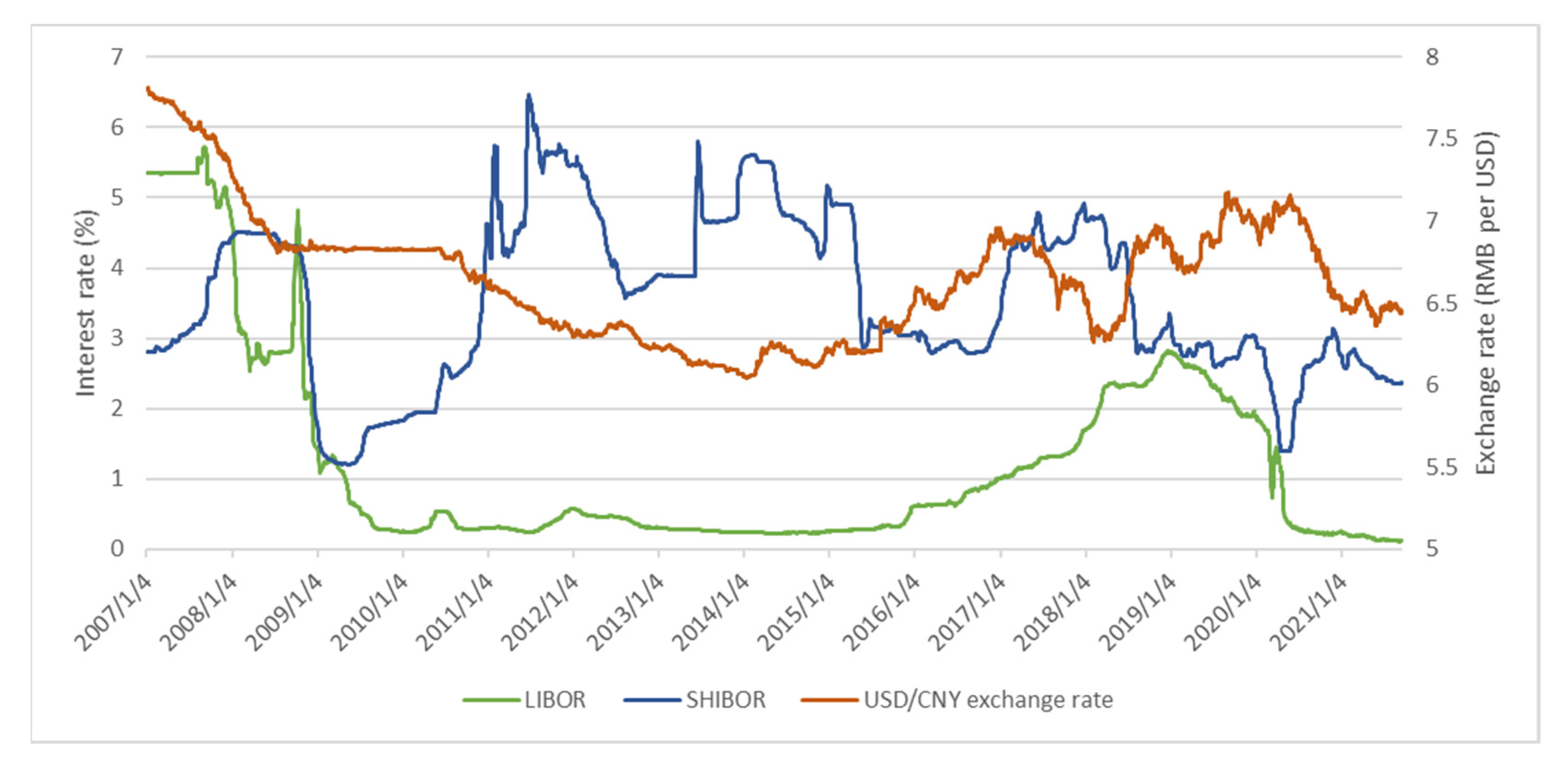
The sufficient wide-interest-rate differential and the favorable exchange-rate movement are two fundamental conditions that support carry trading in RMB. Figure 1 depicts movements of the RMB interest rate, the USD interest rate, and the exchange rate of RMB per USD (right axis) over 2007 January to 2021 September. The three-month Shanghai Interbank Offered Rate (Shibor) is the proxy for the RMB interest rate, and the three-month USD London Interbank Offered Rate (Libor) is the proxy for the USD interest rate. According to Figure 1, after the global financial crisis, the RMB interest rate gradually increased to a high level of 4%, hovered at the high level, and then decreased to around 3% in 2016 and 2018. Meanwhile, the Federal Reserve Board conducted ultra-loose monetary policy such as quantitative easing during the financial crisis, and it cut the federal funds rate near to zero to stimulate the economy’s recovery. Hence, the interest differential between the RMB and the USD became wider and wider after 2010 and only shrunk after 2016 when the Federal Reserve decided to increase the policy rate. During the COVID-19 epidemic period beginning in early 2020, both the RMB and the USD interest rate dropped to a low rate, but Shibor increased soon afterwards.
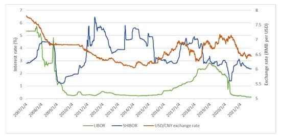
Figure 1.
RMB interest rate, USD interest rate (left axis), and exchange rate of RMB per USD (right axis).
Except to the stable interest differential, investors should also consider the impact of exchange-rate risks on carry-trade returns. Compared to the interest differential, the exchange-rate movement would have a larger effect on carry-trade returns because of their more volatile fluctuations. If the high-interest currency (or investment currency) is in a phase of gradual depreciation, the profit of the carry trade will easily be absorbed by the loss in the exchange rate. Figure 1 also shows the spot exchange rate between the USD and the RMB from January 2007 to September 2021 (right axis). Since 21 July 2005, China has begun to implement a “managed floating exchange rate system based on market supply and demand, with reference to a basket of currencies” and finished the regime’s pegging the RMB solely to the USD. As can be seen from the Figure 1, after China ended its compulsory foreign-exchange settlement-and-sale system in 2007, the RMB began to appreciate gradually against the USD from 2007 to mid-2014.
After the crisis, the quantitative-easing policies adopted by major developed economies have also caused a huge impact on China’s foreign-exchange situation. In order to shield from external risks, China fixed the exchange rate of RMB per USD at around 6.83. Until June 2010, China resumed its exchange-rate reform and ended the two-year system that linked the RMB to the USD. Afterwards, the RMB continued to appreciate unilaterally. On 11 August 2015, the Chinese Central Bank issued a statement on improving the central parity quotation of the exchange rate, which emphasized that the central parity quotation reported to the China Foreign Exchange Trade System should be based on “refer to the closing exchange rate of the interbank foreign exchange market on the previous day, supply and demand in the market, and price movement of major currencies.” Since the 811 reform, the RMB exchange rate has been more market oriented. It can be seen from Figure 1 that, after 2015, the RMB exchange rate against the USD ended the RMB’s unilateral appreciation, and it became a bilateral movement with a wider band.
3.2. Capital Mobility
Cross-border capital flows are the foundation of RMB carry trading. In 1996, the current account was realized as freely convertible in China, but there was strict controls on capital flows of the capital account. From 2013, the Chinese monetary authority gradually introduced systems such as the Qualified Foreign Institutional Investor (QFII), the RMB Qualified Foreign Institutional Investor (RQFII), Shanghai–Hong Kong Stock Connect, the Shenzhen–Hong Kong Stock Connect, and the Shanghai–London Stock Connect in order to increase the degree of China’s capital-market openness. In September 2019, the State Administration of Foreign Exchange announced that it would abolish the investment quota restrictions for QFII and RQFII to further deepen the degree of financial-market openness.
3.3. Realization of the RMB Carry Trade
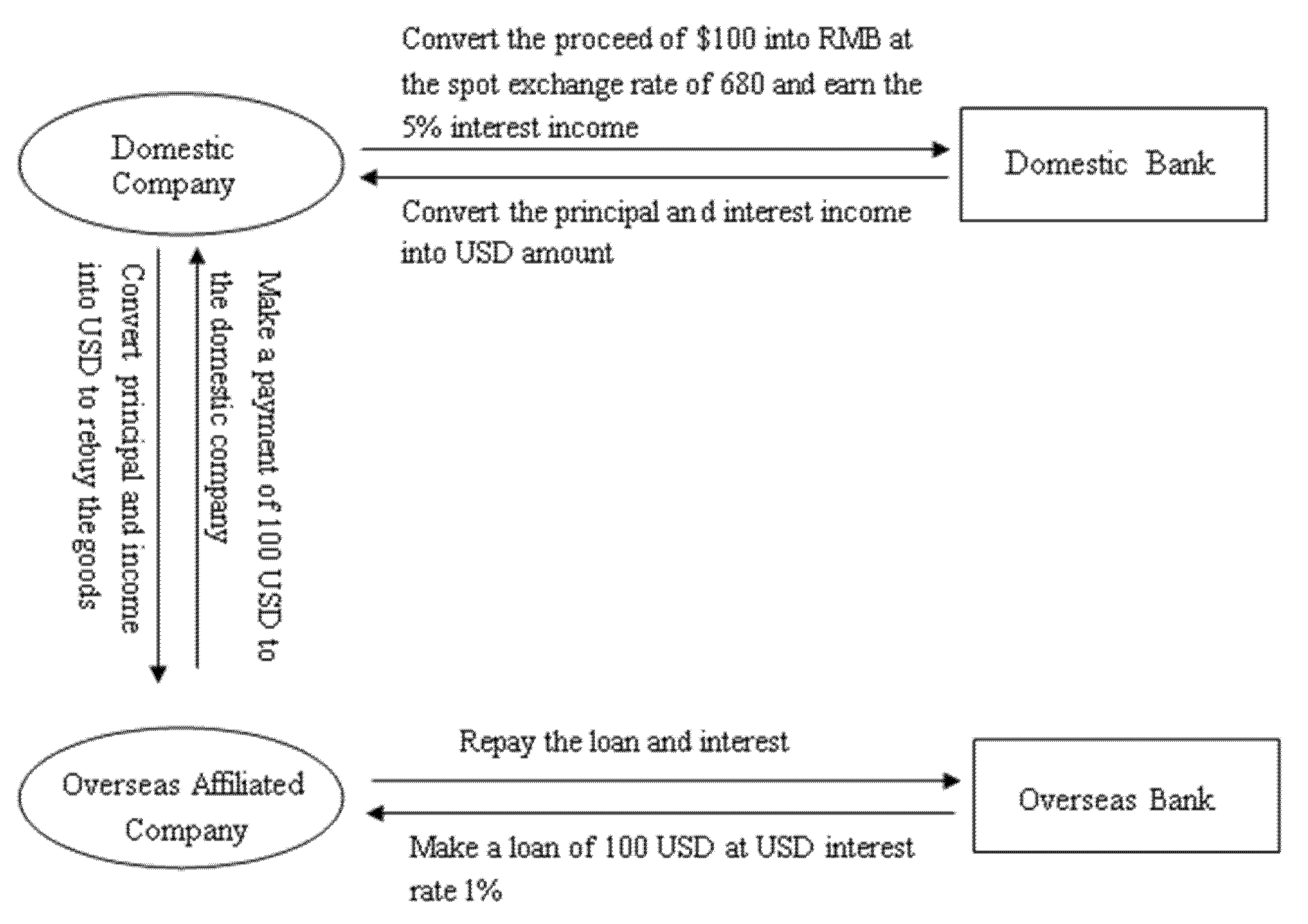
Due to the policy controls on capital flows, the high interest differential could not be quickly wiped out by foreign arbitrage capital. Nowadays, investors could invest in China’s financial market through QFII, RQFII, the Shanghai–Hong Kong Stock Connect, the Shenzhen–Hong Kong Stock Connect, etc. In addition, investors tend to take the RMB carry trade through disguising the carry trade as a flow-of-goods trade. Figure 2 illustrates the procedures of the disguised RMB/USD carry trade, and then we give an example to specifically describe the implementation steps of the virtual trade:
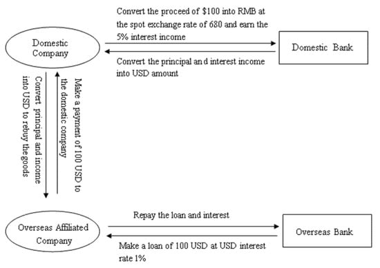
Figure 2.
The illustration of the realization of RMB carry trade.
1. A domestic company exports goods that are worth $100 to an overseas affiliated company.
2. The overseas affiliated company makes a loan on the overseas bank at a 1% USD interest rate and then pays the $100 goods payments to the domestic company. Through this step, the 100 USD amount flows into China as the form of goods payments.
3. After receiving $100 of goods payment, the domestic company converts the USD amount into Chinese Yuan, around 680 RMB (100 × 6.8) at the current spot exchange rate of 6.80 RMB per USD, and invests in RMB-dominating high-interest assets (assuming the RMB interest rate is 5%).
4. At the expiration date of the RMB-dominated investment, the domestic company will receive a total of 714 RMB (680 × 1.05), which includes the principal and the investment income, and then converts the RMB amount to 106.56 USD (714/6.70) at the new spot exchange rate of 6.70 RMB per USD.
5. The overseas affiliated company uses the amount of $106.56 to make up for the loan and the interest—101 USD (100 × 1.01). At the end of the whole process, the domestic company can reap the carry return of approximately 5.56 USD (106.56–101).
4. Model Design
4.1. Constructing the Carry Trade
As mentioned before, after the 2008 global financial crisis, most advanced economies set the policy rate near to zero to stimulate their economies. However, the RMB interest rate still hovered at a high level. Therefore, the wide interest differential between the RMB and other currencies, together with the RMB’s appreciation, made the RMB carry trade attractive. This study assumed the RMB to be an investment currency and chose the USD to be the funding currency. Investors borrow the USD at the USD interest rate and invest in RMB to earn the higher yield, and finally they obtain the excess profits from the RMB carry trade strategy. Therefore, the dependent variable, RMB carry return, was constructed following:
Carry Return () is defined as the profits of the carry trade strategy that longs RMB and shorts USD:
where is the RMB carry return that starts the position at time and ends the position at time ; and are the spot exchange rates of RMB per USD at time and , respectively; and represent the RMB interest rate and USD interest rate from time to time . We used the following form to calculate the carry return:
where and are the logarithmic forms of the spot exchange rates and , respectively. , which means that the RMB depreciates against the USD, and vice versa.
In order to construct a three-month carry trade position, this study selected the three-month Shibor and the three-month USD Libor to be the proxies for the interest rates. Therefore, the time difference between time and was three months, so is the spot interest rate three months later in period , and is the exchange-rate difference among three months (not the daily movement).
4.2. Explanatory Variables
The majority of the existing literature explains the RMB carry return from the perspective of time-varying risk factors, the asynchrony of monetary policies, the peso effect, etc. This study discusses the impact on the RMB carry return of the capital return and the volatility of both the Chinese and the US financial market, the RMB-exchange-crash risk, and the asynchrony of Chinese and US monetary policies. In order to seek variables that have significant long-term and short-term relationships with the RMB/USD carry return, we chose the following variables based on previous studies, and these market-related variables were already stated to be significant in developed economies [5,17,36]:
The Chinese Financial Return (HSret) is measured by the realized daily average return of the Shanghai and Shenzhen 300 Index in the past three months.
The US Financial Return (SPret) is measured by the realized daily average return of the S&P 500 Index in the past three months.
The Chinese Financial Risk (HSrisk) is measured by the realized volatility of the Shanghai and Shenzhen 300 Index daily average return in the past three months.
The US Financial Risk (SPrisk) is measured by the realized volatility of the S&P 500 Index daily average return in the past three months.
The Market Risk Aversion (VIX) is measured by the VIX index. The VIX index is the stock market’s expectation of the S&P 500 index’s volatility and is usually used to measure investors’ sentiments, that is, the level of risk, fear, or stress in the market when making investment decisions. The larger the VIX index, the higher the risk aversion of investors.
The RMB-Exchange-Rate Risk (FXrisk) is measured by the historical volatility of the daily spot exchange rate of the RMB against the USD in the past three months.
The RMB Crash Risk (FXcrash) is measured by the realization skewness of the daily spot exchange rate of the RMB against the USD in the past three months. Due to the characteristics of bilateral exchange rates, the skewness of the USD is the negative skewness of the RMB. The larger the FXcrash value, the more positive the USD skewness, and the more negative the RMB skewness, the greater the RMB crash risk.
The Degree of Policy Differentiation (PD) is measured by the policy rate differential between China and the United States. The US policy interest rate is expressed by the federal funds rate, and China’s policy interest rate is expressed by the seven-day pledged government bond repurchase interest rate.
4.3. Model Specification
To test whether these factors could affect the RMB carry return, this study employed an Auto Regressive Distributed Lag (ARDL) model to conduct the empirical analysis, due to its advantage that estimated coefficients are consistent and efficient with the presence of I(1) series, a small sample, and endogeneity [25,26].
The long-term relationship between the RMB carry return and the selected explanatory variables is expressed by Equation (3):
where is the RMB carry return with the investment horizon from time to time . The right side of Equation (3) is the expected long-term relationship of explanatory variables with carry returns.
It is worth noting that the ARDL model does not simply regress Equation (3) directly. In order to obtain the long-term effect and short-term dynamic relationship between variables, the following error-correction model (ECM) corresponding to the ARDL needs to be estimated, namely:
where is the long-run equilibrium coefficient, is the adjustment speed of the carry return toward the equilibrium level, and is the short-time-dynamic coefficient.
5. Empirical Results
5.1. Data
This study employed daily data from January 2007 to September 2021. The data on the RMB/USD spot exchange rate, the return of the Shanghai and Shenzhen 300 index, and the repurchase rate of China’s seven-day pledge of government bonds are all from the Wind database (the Wind database pairs over 1.3 million macroeconomic and industry time series to give financial professionals the most comprehensive insights into China′s economy). The USD Libor data and the S&P 500 index return data come from the Bloomberg database. Shibor data comes from the official website of the Shanghai Interbank Offered Rate (The official website of SHIBOR: http://www.shibor.org/shibor/web/DataService.jsp) (accessed on 11 November 2021). The VIX data comes from the Chicago Board Options Exchange (CBOE) website—the CBOE is the largest U.S. options exchange, and the CBOE proposed the VIX index. The federal funds rate data comes from the official website of the Federal Reserve Board.
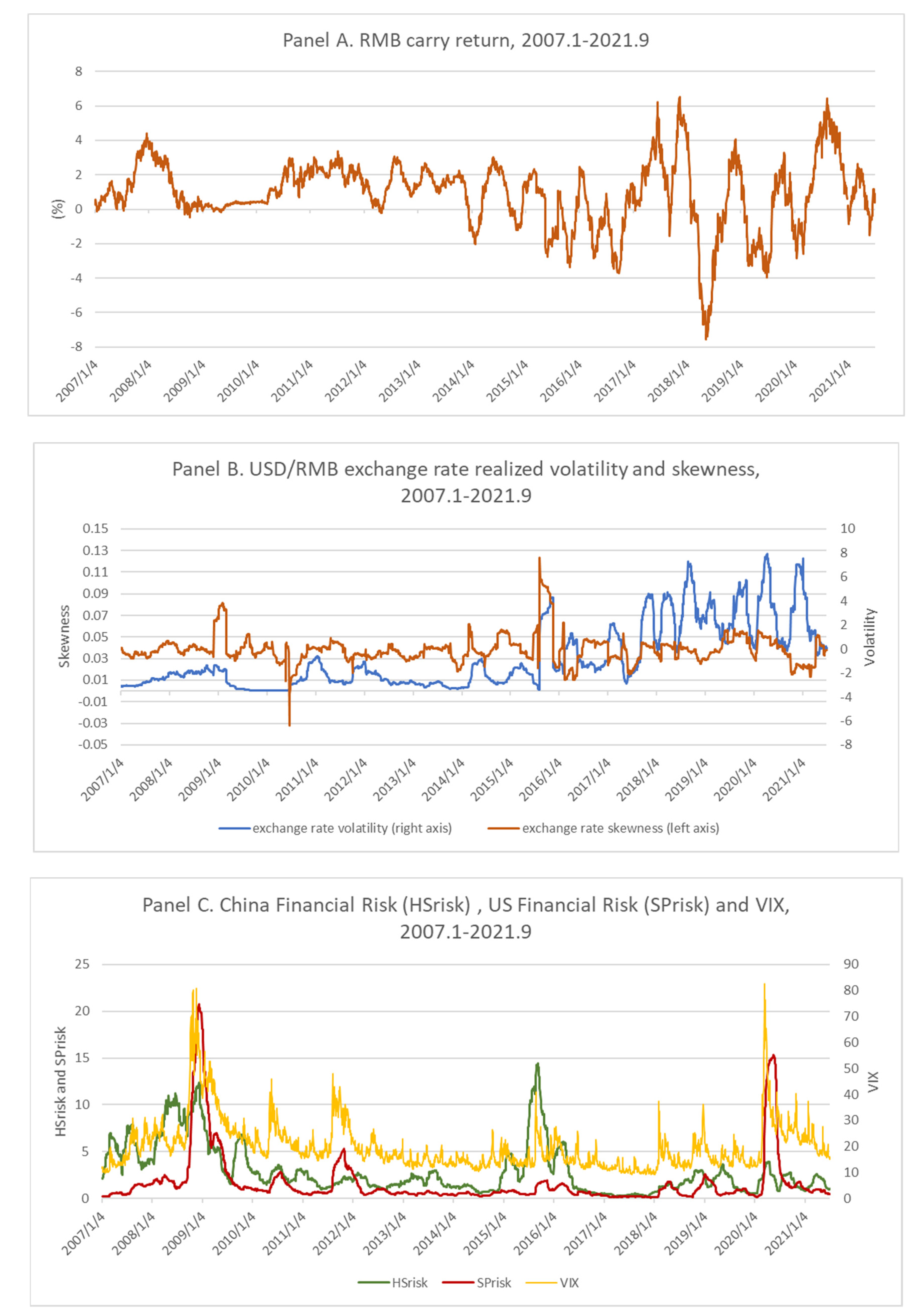
Figure 3 displays the trends of the RMB carry-trade return and other explanatory variables. From panel A, the RMB carry trade steadily hovered above the zero line with little volatility before 2014. After 2015, the RMB carry trade began to perform a more-volatile return and suffered much more losses, and the return’s volatility also increased over time. From panel B, it is obvious that the volatility of the USD/RMB exchange rate became very large after the 811-exchange-rate reform. Panel C displays the three explanatory variables related to China’s financial risk, the US financial market, and the VIX. According to panel C, stock markets showed significant movements in three time periods: during the global financial crisis, all the three variables show large volatility; during the crash period of A shares in 2015, both China’s financial risk and the VIX showed large volatility; during the COVID-19 epidemic period in early 2020, both the US financial risk and the VIX showed large volatility.
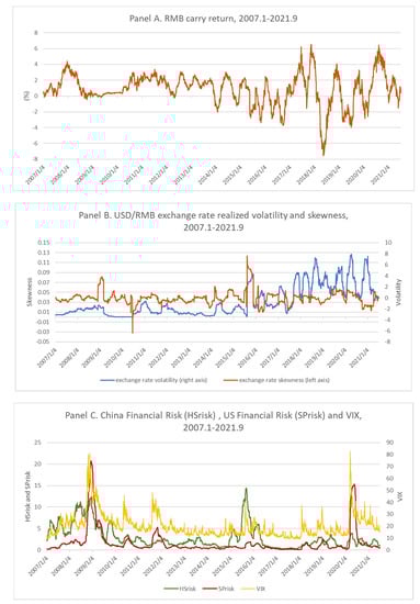
Figure 3.
Statistic description of RMB carry trade and explanatory variables (USD/RMB exchange rate volatility, USD/RMB exchange rate skewness, China’s financial risk, US financial risk, and the VIX).
5.2. Stationary Test
Only the I(0) and I(1) series could be incorporated into the ARDL model, so the stationarity test was performed on all variables before model estimations. Table 1 lists the results of the ADF test and the PP test on the variables. All variables were I(0) or I(1) series, so they can be estimated using ARDL models.

Table 1.
Results of the stationary test.
5.3. RMB/USD UIP Test
The failure of the RMB/USD uncovered interest rate parity provides investors an opportunity to reap profits by carrying out carry trading on RMB/USD. Therefore, we first examine whether UIP holds between RMB and USD. The results of the ARDL regression on the formula are shown in Table 2:
Table 2.
RMB UIP test results through ARDL.
According to Table 2, the interest rate has little explanatory power regarding exchange-rate movements, as the coefficient is not significant. Therefore, the UIP does not hold between the RMB and the USD, and there is an opportunity to obtain a positive return from engaging in the RMB carry trade.
5.4. Model Estimation
The sample horizon was from 2007 to 2021, and the time period included the global financial crisis and the 811-exchange-rate reform. Hence, we divided the time horizon into three sub periods: the global financial crisis (4 January 2007—31 December 2009), before the 811-exchange-rate reform (4 January 2010–11 May 2015), and after the 811-exchange-rate reform (27 August 2015–17 September 2021). We put different explanatory variables into the regression model and selected the best fitted model that optimally explains the carry trade based on the Akaike information criterion (AIC) value and adjusted R-squared for each model. The AIC criterion was chosen instead of the BC criterion, because the AIC criterion prefers models with more lag periods, thus reducing the possibility of any remaining serial correlation in the model.
5.4.1. Bounds Test
Firstly, we needed to conduct a bounds test to judge if the long-run level relationship between the RMB carry return and different explanatory variables exists. According to Pesaran et al. [25], only when the bounds test between variables passes are the estimated coefficients through ARDL and the error-correction model meaningful. The null hypothesis of the bounds test was: , which means that none of explanatory variables had a significant level relationship with the RMB carry return. Table 3 presents the results of the bounds test for three different sub periods. As the table shows, the P value supports the results that the long-run level relationship exists for all those three subperiods, so the following estimated coefficients are meaningful.
Table 3.
Bounds test of interest rate differential and exchange-rate movement.
5.4.2. Parameter Estimation
In order to further discuss the long-term level and the short-term dynamic relationship between the explanatory variables and carry returns, this study estimated the parameters of the error-correction model corresponding to ARDL. For each sub period, we put different combinations of explanatory variables into the regression model. According to each model’s AIC value, the adjusted R-squared, and the parameters’ significance of each model, we selected the optimal one that could explain the carry return. It was necessary to carry out postestimation test of serial autocorrelation and heteroscedasticity on the residual series to ensure that estimated parameters in the model are all efficient. We also tested for the setting error of the regression equation by further testing whether there were other missing variables in the model that can explain carry returns. Finally, we conducted a postestimation normality test.
For the first sub period, the global financial crisis, the optimal model was ARDL (3,0,0,0,0,1,4), and the estimated results are shown in Table 4. As the table shows, the policy differential would have a significant-level relationship with the carry return. The greater the differential between the two policy rates, the higher the carry returns. In terms of the short-term dynamic relationship, the policy differential also had a significant relationship with carry returns. In addition, the crash risk had a significant short-term dynamic relationship with carry returns: when the crash risk increases, the carry returns would increase in the short-term.
Table 4.
Results of estimated coefficient and model test during the global financial crisis.
Based on the results of the model’s postestimation test, we cannot reject the heteroscedasticity of the residual at the level of 5%. The reason for heteroscedasticity is that the RMB carry return changes significantly from the beginning to the end of the global financial crisis period. From Figure 1, the USD depreciates dramatically from 7.8 RMB to 6.8 RMB, so that the vast depreciation causes a bump to the RMB carry trade form September 2007 to September 2008. At the same time, the model’s setting-error test results show that the variables selected in this model could not fully explain the RMB carry return, and there are variables outside the model that can explain the RMB carry return.
Table 5 displays the model-estimation results for the period before the 811-exchange=rate reform. The optimal model was ARDL (4,0,2,0,4,4,0). We incorporated the first-order difference of the volatility of the Shanghai and Shenzhen 300 index () and the S&P 500 index () into the model, representing the change in risk of the Chinese capital market and the US capital market, respectively. As shown in Table 5, changes in the volatility risk in China’s capital market can significantly explain carry returns in the long run: the increase in volatility risks in China’s capital market is accompanied by an increase in RMB carry returns. At the same time, from the perspective of short-term dynamics, changes in capital-market risks have a significant positive relationship with carry returns in the short-term: when the volatility of China’s capital market increases, the current RMB carry return increases significantly. Additionally, in terms of the short-run dynamic, the volatility increase in the US capital market would also significantly increase the current RMB carry-trade return (0.174 **).
Table 5.
Results of estimated coefficient and model test before 811-exchange-rate reform.
In addition, the RMB crash risk could also significantly affect its carry-trade return, which is consistent with findings of Jurek [36], Burnside et al. [37], and Burnside [38]. With the higher crash risk, the RMB exchange rate is more negative-skewed, so carry traders face higher exchange-rate downside risk when they engage in the RMB carry trade. Investors would receive a crash risk premium for holding RMB in a more negative-skewed period and bearing higher crash risk, so there is a significant relationship between crash risk and carry returns in the short run. However, the relationship reverses negatively with more lags. Before the 811-exchange-rate reform, the RMB exchange rate quote was highly close to the USD, and the volatility of the exchange rate was set to be within 1%. Hence, the volatility of the exchange rate (FXrisk) does not have a significant relationship with the carry return.
Table 6 shows the model-estimation results of ARDL (1,0,0,0,2) for the period after the 811-exchange-rate reform. Compared to the results of Table 5, the US-stock-related variables had a weaker impact on the carry trade, so they were not included in the model for the “after-the-exchange-rate-reform” period. As shown in Table 6, China’s capital market return (), market risk (), and investors’ emotion (VIX) could significantly affect the RMB carry return in the long run. When investors’ panic emotion about the market rises, the RMB carry return would increase. The increase in China’s stock market return will weaken the RMB carry return in the long run. Since the majority of carry trades are invested to earn RMB interest-income instruments, the underlying assets are mostly consisted of bonds, debt, etc. When the stock market performs well, the capital flows turn from debt products to the stock market, so the decrease in debt yield will lead to a decrease in carry return. After examining the relationship between the Shanghai and Shenzhen 300 index returns and the bond repurchase rates, this study found that there is indeed a negative correlation between these two asset returns.
Table 6.
Results of estimated coefficient and model test after the 811-exchange-rate reform.
From the perspective of the short-term dynamic relationship, the crash risk could also significantly affect the RMB carry return: with the positive coefficient of (0.212 ***), and a higher RMB crash risk would lead to a higher carry return. Similar with the results of the “before-the-exchange-rate-reform” period, the positive effect would become negative with time, and the estimated coefficient of was significantly lower (−0.111 *).
From Table 6, the results show that the VIX has a significant short-term dynamic and a long-term level relationship with the RMB carry trade. This finding is mainly consistent with those of the related studies [5,10,17]. However, the VIX coefficient has a different sign with the conclusion of Brunnermeier et al. [17] due to the different currency sample and time period. We found a significant negative relationship between China’s financial return () and the RMB carry trade after the 811-exchange-rate reform. This is similar to the finding of Cao [46] that appreciation of the RMB is not an unfavorable factor for the Chinese stock market.
We compared the results of Table 5 and Table 6 to analyze the differences in explaining the RMB carry return before and after the 811-exchange-rate reform. Firstly, the Ramsey RESET test result in Table 5 shows that we rejected the null hypothesis of none of the omitted variables, so there were still omitted variables in the model before the exchange-rate-reform at the 5% level of confidence. However, the Ramsey RESET test results in Table 6 show that we could not reject the no-omitted-variables hypothesis, and variables in the model could already explain the RMB carry return. Secondly, there was only one variable “China’s financial risk” () that had a level relationship with the RMB return before the exchange-rate reform, and three market-related variables had a significant-level relationship with the carry return after the reform. Finally, before the reform, whether it was a long-term level or a short-term dynamic relationship, RMB returns were not affected by market emotion (VIX). As a highly leveraged arbitrage trading strategy, it is rare that the return is not affected by investors’ fear emotion.
The carry trade is an arbitrage investment closely related to the capital market. The carry return should be influenced to a large extent by the capital market. At the same time, theoretically, the carry trade can promote the flow of international funds to economies that can generate higher returns and can drive the exchange rate toward an equilibrium exchange-rate level. However, before the exchange-rate reform, there was no significant relationship between market-related variables (such as market volatility, the VIX, etc.) and RMB carry returns. There are many other non-traditional variables that are related with RMB carry returns before the exchange-rate reform. On the contrary, after the exchange-rate reform, the relationship between the RMB carry return and the capital markets of China has become closer, and the carry return has become traceable. The variables in the model could explain returns significantly and effectively. Therefore, the exchange rate is more market-oriented after the reform, and the RMB carry trade has also played a role in the pricing of the RMB exchange rate. Indeed, through investigating the cross-correlations and the nonlinear causal relationship between the onshore and offshore RMB exchange markets, several studies found that after the 811-exchange-rate reform, the RMB exchange-rate-formation mechanism was effectively improved [47,48].
5.5. Robustness Test
For some countries with capital restrictions, international funds cannot freely flow in and out in large amounts, so carry trades will be carried out through non-deliverable forwards (NDF). When using forward transactions, we assumed covered interest parity (CIP) holds: currency forward discounts with high interest rates to the low interest rates, and the discount rate is exactly the interest differential. Therefore, the future depreciation rate of the forward-discounted currency will be exactly equal to the NDF discount rate under the condition of UIP, otherwise there will be arbitrage space. The NDF carry trade holds a long position in a forward-discount currency and holds a short position in a forward-premium currency at the same time. At the end of the carry trade position, if the depreciation of the forward-discount currency is less than the NDF discount rate (or even the appreciation of the discount currency), the spot value of the long discount currency will be greater than the cost of settlement of the NDF; so, the NDF carry trade receives profits.
In the robustness test, we employed RMB NDF for carry trading. Since the RMB was at a forward discount for most of the time, as in the previous study, the NDF strategy here always holds long RMB forwards and short USD. In the case that the UIP does not hold, the carry-trade return is the difference between the depreciation rate of RMB against USD and the forward discount rate.
NDF Carry Returns (NDF) is expressed by:
where is the RMB NDF carry return that starts the position at time and ends the position at time ; and are the logarithmic forms of the spot exchange rate of RMB per USD at time and , respectively; is the logarithmic forms of the NDF exchange rate at time that settled at time .
We selected the daily data of the three-month NDF exchange rate from January 2007 to September 2021 to engage in the RMB NDF carry trade and conducted a robustness test for the three sub periods. Table 7 shows the results of the robustness test of these three models. First of all, for the regression results during the global financial crisis, the signs of the estimated coefficients were consistent with those of the original model. The variables and coefficients were still significant in the test model. Secondly, in the sub period before the 811-exchange-rate reform, the tested model coefficients were basically the same as the original model, and the regression coefficient signs were in line with expectations. However, in the long-term level relationship, changes in China’s capital-market volatility risk were no longer significant. Finally, the test results after the 811-exchange-rate reform show that the estimated coefficients of the NDF results were consistent with coefficients’ signs and the significance of the previous mode, which are also in line with expectations. Meanwhile, the normality test and the model error test have passed.
Table 7.
Robustness test results.
6. Conclusions
Using the ARDL model, this study investigated the factors that will affect the RMB carry return sustainably. It concludes that during three time periods, the factors affecting the carry trade are different. Comparing the empirical results before and after the 811-exchange-rate reform, we found that the sources of the RMB carry-trade return after the exchange-rate reform have become more traceable. Market-related variables can explain the RMB carry return significantly in the long-term equilibrium, and the model has a higher degree of fitness and fewer missing variables. This indicates that after the exchange-rate reform, the RMB exchange-rate-formation mechanism is more market-oriented and the RMB carry return becomes more explainable. The carry trade could correct the inaccurate pricing in the market, so that the RMB carry trade can give better play to its pricing role after the exchange-rate reform. According to these findings, this study provides the following suggestions:
Firstly, monetary authorities could increase the cost of rapid capital withdrawal, which is conducive to slowing down the withdrawal of speculative capital and to reducing the noise caused by the unwinding of the carry trade to the economy.
Secondly, monetary authorities, especially in developing countries, could reduce restrictions on foreign-exchange movements to lower the expectation of speculators. Once carry traders face higher risks and uncertainty, they would hold the carry trade more prudently. It would avoid the price bubble caused by the surge into the high-yield currency and the crash risk caused by the carry positions’ sudden liquidation.
Finally, for China’s market, the central bank could promote the reform of the RMB exchange-rate mechanism steadily, and the central bank could promote the carry trade to correct the inaccurate pricing of the RMB exchange rate.
Author Contributions
Conceptualization, Z.Z.; methodology, Z.Z.; software, Z.Z.; validation, Z.Z.; formal analysis, Z.Z.; investigation, Z.Z.; resources, Z.Z.; data curation, Z.Z.; writing—original draft preparation, Z.Z.; writing—review and editing, Z.Z. and S.G.; visualization, Z.Z.; supervision, S.G.; project administration, Z.Z. All authors have read and agreed to the published version of the manuscript.
Funding
This research received no external funding.
Institutional Review Board Statement
Not applicable.
Informed Consent Statement
Not applicable.
Data Availability Statement
Restrictions apply to the availability of these data. RMB/USD spot exchange rate, Shanghai and Shenzhen 300 return, and the repurchase rate of China’s seven-day pledge of government bonds data are available from: https://www.wind.com.cn/newsite/wft.html (accessed on 11 November 2021) with the permission of the Wind. VIX data is publicly available and can be found here: https://www.cboe.com/tradable_products/vix/vix_historical_data/ (accessed on 11 November 2021). Shibor data is publicly availa-ble and can be found here: http://www.shibor.org/shibor/web/DataService.jsp (accessed on 11 November 2021). The federal funds rate data is publicly available and can be found here: https://www.federalreserve.gov/data.htm (accessed on 11 November 2021).
Acknowledgments
The authors would like to thank He Liping of the Business School of Beijing Normal University for helpful discussions on topics related to this work.
Conflicts of Interest
No conflict of interest exists in this manuscript, and the manuscript was approved by all authors for publication. The work described was original research that has not been published previously and is not under consideration for publication elsewhere, in whole or in part. All the authors listed have approved the manuscript that is enclosed.
References
- Berg, K.A.; Mark, N.C. Global macro risks in currency excess returns. J. Empir. Financ. 2018, 45, 300–315. [Google Scholar] [CrossRef] [Green Version]
- Berg, K.A.; Mark, N.C. Measures of global uncertainty and carry-trade excess returns. J. Int. Money Financ. 2018, 88, 212–227. [Google Scholar] [CrossRef]
- Engel, C.; Lee, D.; Liu, C.; Liu, C.; Wu, S.P.Y. The uncovered interest parity puzzle, exchange rate forecasting, and Taylor rules. J. Int. Money Financ. 2019, 95, 317–331. [Google Scholar] [CrossRef] [Green Version]
- Galí, J. Uncovered interest parity, forward guidance and the exchange rate. J. Money Credit. Bank. 2020, 52, 465–496. [Google Scholar] [CrossRef]
- Menkhoff, L.; Sarno, L.; Schmeling, M.; Schrimpf, A. Carry trades and global foreign exchange volatility. J. Financ. 2012, 67, 681–718. [Google Scholar] [CrossRef] [Green Version]
- Ilut, C. Ambiguity aversion: Implications for the uncovered interest rate parity puzzle. Am. Econ. J. Macroecon. 2012, 4, 33–65. [Google Scholar] [CrossRef] [Green Version]
- Colacito, R.; Croce, M.M. International asset pricing with recursive preferences. J. Financ. 2013, 68, 2651–2686. [Google Scholar] [CrossRef] [Green Version]
- Brunnermeier, M.K.; Pedersen, L.H. Market liquidity and funding liquidity. Rev. Financ. Stud. 2009, 22, 2201–2238. [Google Scholar] [CrossRef] [Green Version]
- Farhi, E.; Fraiberger, S.P.; Gabaix, X.; Ranciere, R.; Verdelhan, A. Crash Risk in Currency Markets; National Bureau of Economic Research: Cambridge, MA, USA, 2009; pp. 898–2937. [Google Scholar]
- Ismailov, A.; Rossi, B. Uncertainty and deviations from uncovered interest rate parity. J. Int. Money Financ. 2018, 88, 242–259. [Google Scholar] [CrossRef]
- Fama, E.F. Forward and spot exchange rates. J. Monet. Econ. 1984, 14, 319–338. [Google Scholar] [CrossRef]
- Li, D.; Ghoshray, A.; Morley, B. Uncovered Interest Parity and the Risk Premium; Working Paper; University of Bath, Department of Economics: Bath, UK, 2011. [Google Scholar]
- McCallum, B.T. A reconsideration of the uncovered interest parity relationship. J. Monet. Econ. 1994, 33, 105–132. [Google Scholar] [CrossRef] [Green Version]
- Lin, S.; Xiao, J.; Ye, H. Disguised carry trade and the transmission of global liquidity shocks: Evidence from China’s goods trade data. J. Int. Money Financ. 2020, 104, 102180. [Google Scholar] [CrossRef]
- Zhang, M.; Balding, C. Carry Trade Dynamics under Capital Controls: The Case of China. 2015. Available online: https://ssrn.com/abstract=2623794 (accessed on 7 November 2021).
- Zhao, W. RMB Carry Trade, Commodity Carry and Trade Imbalance of China. Ph.D. Thesis, Central University of Finance and Economics, Beijing, China, 2017. (In Chinese). [Google Scholar]
- Brunnermeier, M.K.; Nagel, S.; Pedersen, L.H. Carry trades and currency crashes. NBER Macroecon. Annu. 2008, 23, 313–348. [Google Scholar] [CrossRef] [Green Version]
- Plantin, G.; Shin, H.S. Carry Trades, Monetary Policy and Speculative Dynamics. 2011. Available online: https://ssrn.com/abstract=1758433 (accessed on 7 November 2021).
- Fratzscher, M. What explains global exchange rate movements during the financial crisis? J. Int. Money Financ. 2009, 28, 1390–1407. [Google Scholar] [CrossRef] [Green Version]
- Gagnon, J.; Chaboud, A. What can the data tell us about carry trades in Japanese yen? 2007. Available online: https://ssrn.com/abstract=1006193 (accessed on 7 November 2021).
- Melvin, M.; Taylor, M.P. The crisis in the foreign exchange market. J. Int. Money Financ. 2009, 28, 1317–1330. [Google Scholar] [CrossRef] [Green Version]
- Ahmed, S.; Zlate, A. Capital flows to emerging market economies: A brave new world? J. Int. Money Financ. 2014, 48, 221–248. [Google Scholar] [CrossRef] [Green Version]
- Aizenman, J.; Binici, M.; Hutchison, M.M. The Transmission of Federal Reserve Tapering News to Emerging Financial Markets. Int. J. Cent. Bank. 2016, 12, 317–356. [Google Scholar]
- Korinek, A. Regulating capital flows to emerging markets: An externality view. J. Int. Econ. 2018, 111, 61–80. [Google Scholar] [CrossRef] [Green Version]
- Pesaran, M.H.; Shin, Y.; Smith, R.J. Bounds testing approaches to the analysis of level relationships. J. Appl. Econom. 2001, 16, 289–326. [Google Scholar] [CrossRef]
- Nkoro, E.; Uko, A.K. Autoregressive Distributed Lag (ARDL) cointegration technique: Application and interpretation. J. Stat. Econom. Methods 2016, 5, 63–91. [Google Scholar]
- Zheng, L. Does 811 Exchange Rate Reform Enhance the Market-Orientation and Benchmark Status of the Central Parity Rate? J. Financ. Res. 2017, 4, 1–16. [Google Scholar]
- Londono, J.M.; Zhou, H. Variance risk premiums and the forward premium puzzle. J. Financ. Econ. 2017, 124, 415–440. [Google Scholar] [CrossRef] [Green Version]
- Yung, J. Can interest rate factors explain exchange rate fluctuations? J. Empir. Financ. 2021, 61, 34–56. [Google Scholar] [CrossRef]
- Ready, R.; Roussanov, N.; Ward, C. Commodity trade and the carry trade: A tale of two countries. J. Financ. 2017, 72, 2629–2684. [Google Scholar] [CrossRef]
- Lustig, H.; Roussanov, N.; Verdelhan, A. Countercyclical currency risk premia. J. Financ. Econ. 2014, 111, 527–553. [Google Scholar] [CrossRef] [Green Version]
- Lustig, H.; Roussanov, N.; Verdelhan, A. Common risk factors in currency markets. Rev. Financ. Stud. 2011, 24, 3731–3777. [Google Scholar] [CrossRef]
- Shen, J.; Sun, X.; Chen, H. Who is the protagonist of explaining the excess returns of carry trade?--Based on the empirical evidence of decomposing volatility risk. Int. Financ. Res. 2020, 7, 77–86. (In Chinese) [Google Scholar]
- Della Corte, P.; Ramadorai, T.; Sarno, L. Volatility risk premia and exchange rate predictability. J. Financ. Econ. 2016, 120, 21–40. [Google Scholar] [CrossRef]
- Schmitt-Grohé, S.; Uribe, M.; Ramos, A. International Macroeconomics; Duke University: Durham, NC, USA, 2008. [Google Scholar]
- Jurek, J.W. Crash-neutral currency carry trades. J. Financ. Econ. 2014, 113, 325–347. [Google Scholar] [CrossRef] [Green Version]
- Burnside, C.; Eichenbaum, M.; Kleshchelski, I.; Rebelo, S. Do peso problems explain the returns to the carry trade? Rev. Financ. Stud. 2011, 24, 853–891. [Google Scholar] [CrossRef]
- Burnside, C. Carry Trades and Risk. In Handbook of Exchange Rates; James, J., Marsh, I.W., Sarno, L., Eds.; John Wiley and Sons: Hoboken, NJ, USA, 2011. [Google Scholar]
- Rafferty, B. Currency Returns, Skewness and Crash Risk; Duke University, 2012; Available online: https://ssrn.com/abstract=2022920 (accessed on 7 November 2021). [CrossRef] [Green Version]
- Atanasov, V.; Nitschka, T. Currency excess returns and global downside market risk. J. Int. Money Financ. 2014, 47, 268–285. [Google Scholar] [CrossRef] [Green Version]
- Mancini, L.; Ranaldo, A.; Wrampelmeyer, J. Liquidity in the Foreign Exchange Market: Measurement, Commonality, and Risk Premiums. J. Financ. 2013, 68, 1805–1841. [Google Scholar] [CrossRef] [Green Version]
- MacDonald, R.; Nagayasu, J. Currency forecast errors and carry trades at times of low interest rates: Evidence from survey data on the yen/dollar exchange rate. J. Int. Money Financ. 2015, 53, 1–19. [Google Scholar] [CrossRef]
- Abankwa, S.; Blenman, L.P. Measuring liquidity risk effects on carry trades across currencies and regimes. J. Multinatl. Financ. Manag. 2021, 60, 100683. [Google Scholar] [CrossRef]
- Serdengeçti, S.; Sensoy, A.; Nguyen, D.K. Dynamics of return and liquidity (co) jumps in emerging foreign exchange markets. J. Int. Financ. Mark. Inst. Money 2021, 73, 101377. [Google Scholar] [CrossRef]
- Lustig, H.; Verdelhan, A. The cross section of foreign currency risk premia and consumption growth risk. Am. Econ. Rev. 2007, 97, 89–117. [Google Scholar] [CrossRef] [Green Version]
- Cao, G. Time-varying effects of changes in the interest rate and the RMB exchange rate on the stock market of China: Evidence from the long-memory TVP-VAR model. Emerg. Mark. Financ. Trade 2012, 48 (Suppl. S2), 230–248. [Google Scholar] [CrossRef]
- Qin, J. Relationship between onshore and offshore renminbi exchange markets: Evidence from multiscale cross-correlation and nonlinear causal effect analyses. Phys. A Stat. Mech. Its Appl. 2019, 527, 121183. [Google Scholar] [CrossRef]
- Xing, W.; Xueping, N.; Fuyou, L. Empirical Test of the Relationship between Renminbi NDF and Onshore Renminbi Exchange Rate. Manag. Rev. 2020, 32, 81. [Google Scholar]
Publisher’s Note: MDPI stays neutral with regard to jurisdictional claims in published maps and institutional affiliations. |
© 2021 by the authors. Licensee MDPI, Basel, Switzerland. This article is an open access article distributed under the terms and conditions of the Creative Commons Attribution (CC BY) license (https://creativecommons.org/licenses/by/4.0/).