1. Introduction
Electricity is a fundamental right worldwide, and all national governments and multiple independent organizations strive together to make this public service universally accessible [
1,
2]. However, this involves a colossal challenge: most countries use fossil fuels to generate electricity, which directly affects us, as the emission of environmental pollutants into the atmosphere leads to global warming [
3,
4]. Therefore, to extend electricity coverage and mitigate greenhouse gas emissions, most governments have created policies to motivate the electricity sector to invest in dispersed generation on a massive and integrated scale, mainly based on photovoltaic (PV) and wind technology [
5,
6,
7]. In the Colombian context, in 2014, the Senate of the Republic approved the 1715 Law, which regulates the integration of dispersed generation into the electricity distribution sector [
8,
9]. This law has significantly promoted the usage of renewable resources in urban and rural areas [
10]; however, today, there exists in multiple regions of Colombia the unique possibility of generating electricity energy through diesel generators [
11]. The most recent report (31 August 2021) of the Institute for Promoting Electricity Solutions in Non-Interconnected Areas (IPSE is the abbreviation for its Spanish name) shows the usage of diesel sources in Colombia compared with the incipient integration of renewable energies [
12]. Currently, the total diesel generation capacity is about 267,911 kW, which benefits about 201,412 users, whereas for solar PV generation, the installed capacity is 21,710 kW, which benefits about 23,617 users. These values show that PV energy supplies less than 10% of the users that diesel sources do [
12].
Figure 1 and
Figure 2 show the current state of the diesel and PV generation in Colombia.
The distributions of diesel generation and PV generation show that in Colombia, similarly to the cases of the Caribbean and Pacific regions, the potential of several solar resource-rich regions has not been realized [
13]; however, this problem can be solved using sustainable energy solutions [
11].
The possibility of integrating PV sources in countries such as Colombia is a certainty; nevertheless, after identifying promising areas where these solutions can provide clean energy to thousands of end-users [
14], efficient optimization techniques that permit their optimal siting and sizing in the distribution network need to be proposed [
15]. These solution strategies must consider economic and technical aspects. The economic considerations should include the generation costs of conventional sources and the investment and operating costs of PV sources [
16]. The technical aspects should encompass voltage regulation and power balance equilibrium in all nodes of the network [
17,
18], among others.
To address the problem of the optimal placement and sizing of PV sources in electrical distribution networks, an objective function is proposed herein that involves the simultaneous minimization of the grid generation costs of conventional sources and the investment and operating costs of PV sources for a planning period of 20 years. The proposed optimization model is from the family of mixed-integer nonlinear programming (MINLP). For this reason, a discrete–continuous version of the Chu and Beasley genetic algorithm (DCCBGA), recently proposed in [
19] to locate and size distribution static compensators, was employed in this study to solve the complete MINLP model.
In the literature, multiple optimization approaches can be found that aim to solve the problem of the optimal locations of dispersed generators in electrical distribution grids. Some of these approaches include particle swarm optimization [
20], genetic algorithms [
21], the sine–cosine algorithm [
22], the population-based incremental learning optimizer [
17], krill herd optimization [
23], the vortex-search algorithm [
15], and mathematical-based approaches in the General Algebraic Modeling System (GAMS) [
24,
25]. The main characteristic of these approaches is that the objective function considered is typically associated with the minimization of total grid losses in the peak hour condition, which is an unrealistic simulation case, owing to the fact that the loads and the renewables vary their behavior over the day [
15].
Some of the literature has addressed the multi-period problem in distribution networks with renewable energies and batteries as follows: The authors of [
16] proposed that battery energy storage systems and renewable generation in medium- and low-voltage distribution grids be optimally integrated. The problem was decoupled into two stages. A heuristic algorithm based on simulated annealing defined the locations of the distributed energy resources, and mixed-integer linear programming defined their optimal daily outputs. The numerical results of the test feeders composed of 11, 135, and 230 nodes demonstrated the efficiency of the proposed approach when compared with conic models. The authors of [
26] studied the problem of the optimal siting and sizing of wind energy sources in distribution and transmission systems. They solved the exact MINLP model with the help of the GAMS optimization package. Their main contribution was the discovery of the reactive power capabilities of wind turbines to minimize grid energy losses. The main problem of the study is that the authors did not take into account costs in the objective function, which means that that the devices might have been over-sized. The same approach by the authors of [
26] was extended in [
27] to high-voltage transmissions networks while considering PV generators with dynamic active and reactive power capabilities. The exacted MINLP model was also solved in the GAMS environment; however, the investment and operating costs for renewables were not considered. Molina et al. in [
28] proposed a convex optimization model based on second-order cone programming to minimize the total greenhouse gas emissions in distribution networks in rural areas by integrating PV sources. The proposed optimization approach ensures finding the global optimum; however, the authors did not include the economic aspects in the optimal sizing problem, which limits the applicability of their solution to real distribution grids.
With respect to the state-of-the-art research just mentioned, the main contributions of this study are the following:
The formulation of an MINLP model that represents the problem of the optimal siting and sizing of PV sources in grid-connected distribution networks with the aim of minimizing the total energy purchasing costs in the substation bus and the investment and operating costs of the PV sources for a planning horizon of 20 years.
The solution of the MINLP model through an application of the DCCBGA, which has not been previously used for the studied problem. Numerical results demonstrated its superior performance when compared with the GAMS software in terms of response quality and convergence guarantee.
It is worth mentioning that the proposed study did not consider the presence of battery energy storage systems or controllable and referable loads, as we were interested in exploring solar solutions for grid-connected areas with minimum investment costs. However, the inclusion of these devices is an opportunity for future research [
29,
30]. Regarding the selection of the classical Chu and Beasley genetic algorithm (CBGA) and its discrete–continuous version of codification, which helps solve the problem of the optimal location and sizing of PV sources with a unified vector: it is important to say that this optimization algorithm was selected to solve the proposed MINLP model, as it is a widely known model and is used to solve complex optimization problems with efficient numerical performance and low computational effort. Moreover, the discrete–continuous version of the CBGA has recently yielded satisfactory results for the optimal reactive compensation problems, as reported in [
19] for static compensators and in [
31] for optimal reactive power flow in transmission systems.
The remainder of this research is organized as follows:
Section 2 presents the general optimization model for the optimal location and sizing of PV sources in grid-connected distribution networks considering investment and operating costs for a planning period with
years.
Section 3 presents the main aspects of the proposed optimization methodology, which is guided in the master stage by the DCCBGA, which uses the recursive solution of the power flow problem in the slave stage with the successive approximation power flow approach.
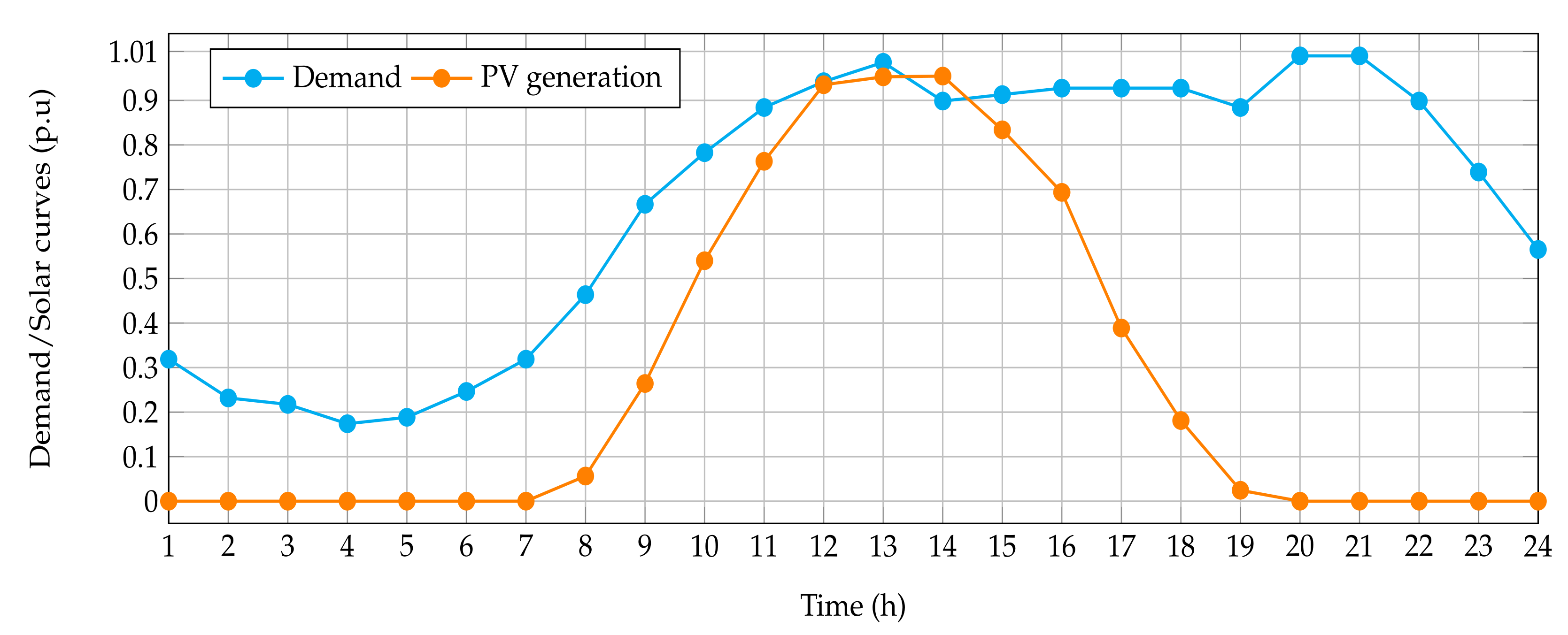
Section 4 describes the main features of the IEEE 33-bus and IEEE 69-bus systems, including their load and branch parameters. It also presents the load generation and demand curves and the necessary parameters for evaluating the objective function.
Section 5 presents the computational validation of the proposed methodology with the GAMS optimization package in both test feeders. Finally,
Section 6 lists the main conclusions derived from this project and some recommendations for future studies.
3. Proposed Solution Methodology
To deal with the problem of the optimal placement and sizing of PV sources in grid-connected distribution grids, in this study, we propose the application of the DCCBGA [
33]. The main advantage of this approach is that the proposed codification defines the optimal locations and sizes of the PV sources in a unique vector, which reduces one stage in the classical optimization methods, where an additional optimization algorithm is used to define their sizes [
34].
The proposed codification has the following structure:
where its dimensionality is
. The first
is associated with the nodes where the PV sources will be installed (discrete part of the codification), and the second relates to their optimal sizes (continuous part of the codification). Note that with the usage of this codification, the proposed optimization methodology is composed of two stages, which are the master stage guided by the CBGA, and the slave optimization stage, where a power flow is used to evaluate the first component of the objective function, i.e., the total energy purchasing costs in the conventional sources. The main characteristics of the master and slave optimization stages are illustrated in
Figure 3.
As previously mentioned, the master stages are entrusted with guiding the exploration and exploitation of the solution space through the application of the evolution criteria to an initial population; however, to know the value of the fitness function (objective function plus penalizations), the use of a slave stage entrusted with solving the multiperiod power flow problem is required. Each stage is presented in detail below.
3.1. Master Optimization Stage
The master optimization stage can be defined as the brain of the solution methodology, as this is entrusted with defining the best set of candidate solutions with the structure presented in (
12). This is done by applying different evolution criteria, which, in turn, is done by initializing these solutions with a random procedure that ensures their optimal dispersion in the solution space. In the flowchart presented in
Figure 4, the main aspects of the proposed DCCBGA to define the optimal placement and sizing of PV sources in grid-connected distribution systems are summarized.
From
Figure 4, which describes the general implementation of the proposed DCCBGA, we can note the following:
- 🗸
The initial population is generated randomly in the solution space using a Gaussian distribution with normal form. This initial population corresponds to a matrix with
rows, each of them with the structure presented in Equation (
12).
- 🗸
The slave stage is the heart of the optimization methodology, as it allows the fitness function of the initial population and the offspring population to be known. This stage is presented in detail in the following section.
- 🗸
The tournament is avoided by directly selecting two parents from the population. In addition, the recombination and the mutation criteria are applied for both offspring with 100% probability.
- 🗸
Both mutated offspring are evaluated in the slave stage, and the best individual (lower fitness function value) is selected with the opportunity to become part of the current population if the diversity criterion is fulfilled and its fitness function is at least better than the worst parent in the population.
For additional details regarding the implementation of the CBGA in optimization, refer to the references [
33,
34].
3.2. Slave Stage: Power Flow Solution
The slave stage, as previously mentioned, corresponds to the heart (core) of the optimization strategies based on metaheuristics, as this allows the exploration and exploitation of the solution space to be guided [
34]. In the case of the optimal siting and sizing of PV sources in the solution space, the slave stage is defined by the recursive evaluation of the power flow problem [
17]. Here, we adopt the successive approximations power flow method initially proposed by Montoya and Gil-González in [
35]. The main advantage of this power flow approach is that its numerical convergence can be ensured through the application of the Banach fixed-point theorem [
36].
The general recursive power flow formula based on the successive approximation power flow method takes the following form:
where
m is the iterative counter;
is a complex vector that contains all the voltage variables in the demand nodes (for
, it is assumed that
);
and
are admittance matrices that relate demand and slack nodes among them;
is a complex vector that contains all the power injections in the PV sources;
is a complex vector that contains all the constant power consumptions in the demand nodes;
represents the complex voltage outputs in the slack nodes (this value is perfectly known for power flow studies). Note that operator
becomes the vector
Z in a diagonal matrix;
represents the complex conjugate value of the vector
Z.
Note that the evaluation of the recursive formula (
13) is made until the difference between both consecutive voltages fulfills the convergence criterion, i.e.,
where
is the convergence error, which, as recommended in [
35], is assigned as
.
It is worth mentioning that the master stage for each solution individual in the current population sends the values of the to evaluate the power flow problem and determine its corresponding fitness function value.
In the case of the calculation of the active power injections in the slack node, once the power flow problem is evaluated for each period of time, then, the complex power injection in the slack source (i.e.,
) is calculated as follows:
Once the power flow problem is solved for each period of time as defined in (
13) and the complex power generation in the slack node is calculated, the fitness function is assigned for each individual. The fitness function helps with the evolution of the optimization algorithm to find the minimum value of the objective function that is always feasible. The fitness function (
) in this study takes the following form:
where
and
are the penalization factors associated with the violation of the voltage regulation bounds, which generates an adaptive penalization as a function of the deviation value regarding the lower and upper voltage bounds. Note that the fitness function is equal to the objective function when all the constraints in the mathematical model (
1)–(
11) are fulfilled.
It is worth mentioning that the maximum and minimum power generation bounds of the PV sources are always ensured with the proposed codification of the DCCBGA, and the active and reactive power generation bounds in the slack source are not considered, as these are assumed to have enough capabilities to support all demands even if no PV sources are located on the grid.
5. Numerical Validation
The solution of the MINLP model defined from (
1)–(
11) was implemented in the GAMS software with the solvers BONMIN and COUENNE and with the MATLAB programming environment using its own scripts. In the case of the MATLAB implementations, its
version was used on a PC with an AMD Ryzen 7 3700
GHz processor and 16.0 GB RAM, running on a 64 bit version of Microsoft Windows 10 Single Language.
To verify that the GAMS and MATLAB models are completely equivalent, we evaluated the benchmark case for both test feeders in both programming environments. All the numerical results for the these test feeders are reported below.
5.1. Results for the IEEE 33-Bus System
Table 5 presents the numerical results of the proposed DCCBGA and the GAMS solvers and the benchmark case. Note that the COUENNE solver diverged after 3600.37 s of exploration of the solution space. In the case of the BONMIN solver, it reached the solution in 3.64 s, whereas the proposed DCCBGA took about 5.30 s to solve the MINLP model (
1)–(
11).
The numerical results in
Table 5 show the following: (i) The BONMIN solver in GAMS got stuck in a local optimal solution where nodes 17, 18, and 33 were selected as the best optimal positions with a total installed power capacity of
kWp. (ii) The solution of the DCCBGA is a better optimal solution with an additional improvement of the objective function by about US
$1891.85 per year of operation with respect to the BONMIN solution. The optimal locations identified by the DCCBGA correspond to the nodes 11, 15, and 30, with a total installed power capacity of
kWp. Note that the DCCBGA solution installs
kWp of generation less than the BONMIN solution, which reduces the annualized investment and energy purchasing cost by about US
$7477.48 with respect to the BONMIN solution. (iii) In terms of percentages, the BONMIN solution allows a reduction in the annual grid costs by about 26.99% (i.e., about US
$998,631.24), whereas the improvement of the proposed DCCBGA is
%, i.e., US
$1,000,523.09 per year of operation.
To validate the effectiveness and robustness of the DCCBGA for the studied problem, 100 consecutive evaluations of the the methodology were performed. These evaluations yielded the following results: a minimum objective function value of US
$/year 2,699,932.29, a mean value of US
$/year 2,702,178.35, and a maximum value of US
$/year 2,705,870.99. Note that the standard deviation obtained by our proposal was
dollars, which means that all the solutions were mainly concentrated in a ball with a small radius with respect to the mean value. The efficiency of the proposed DCCBGA for solving the MINLP model (
1)–(
11) is depicted in
Figure 7; the solutions were normalized by the optimal solution obtained by the BONMIN solver. This graphic shows that 44 solutions with better numerical performance than the BONMIN solver were produced, which means that the proposed DCCBGA ensures, with 44% probability, the finding of a better solution when compared with the BONMIN solution in the IEEE 33-bus system.
To illustrate the effect of the PV generation in the generation output on the slack bus,
Figure 7 compares the power generation in the slack node in the benchmark case with the values provided by the DCCBGA and BONMIN solvers.
The behavior of the power output in the slack source depicted in
Figure 8 shows, as expected, that in the benchmark case, the total generation in the slack source followed the aggregated demand curve in the substation terminals. However, when PV sources were installed with the proposed DCCBGA and/or using the BONMIN solution, the well-known duck curve was obtained, which allows the slack generation to be minimized in the time periods where enough PV energy is available [
39].
To verify that the fitness function proposed ensures that the voltage profiles are within
of the optimum,
Figure 9 reports the minimum and maximum voltages obtained at each period of time.
From
Figure 9 it is possible to note that for all periods of time, the voltage profile of the network fulfills the imposed upper and lower regulation bounds (all the voltage magnitudes must be contained between the upper and lower curves presented in
Figure 9). In addition, when the amount of PV power injection is significant, there are some periods where few nodes have voltage magnitudes more than the slack source with a maximum value of
pu, and the minimum voltage value is as expected when the active and reactive power demand is maximum and the PV power injection is zero, i.e., in the time period 20 with a value of
pu.
5.2. Results for the IEEE 69-Bus System
Table 6 presents the numerical results of the proposed DCCBGA for the IEEE 69-bus system. It is worth mentioning that both GAMS solvers diverged after more than one hour of solution space exploration, whereas the proposed DCCBGA took about 22.36 s to solve the MINLP model (
1)–(
11).
Note that the optimal sites to assign PV sources in the IEEE 69-bus system, as presented in
Table 6, are the nodes 24, 61, and 64 with a total installed power capacity of
kWp. These power injections in the nominal operative conditions allow the total grid operative costs to be reduced by about
with respect to the benchmark case.
It is worth mentioning that after 100 consecutive evaluations of the proposed DCCBGA, the following values were obtained: a minimum value of US$/year 2,825,783.32, a maximum value of US$/year 2,844,469.50, a mean value of US$/year 2,829,498.36, and a standard deviation of US$/year . These values imply the following: (i) All the solutions are near to the mean value, concentrated inside of a ball with a radius less than 3000 dollars. (ii) The minimum annual reduction in the operation costs is % for the maximum solution provided by the DCCBGA. (iii) The difference between the extreme solutions obtained by the DCCBGA is US$/year 18,686.18, i.e., less than 0.48% of the total annual operative costs in the benchmark case.
Figure 10 shows the percentage of efficiency reached by the DCCBGa when all the solutions were normalized to the mean value. This plot allows one to observe that there exist 55 solutions that ensure values lower than the mean value, i.e., annual operating costs of US
$/year 2,829,498.36, which implies that the proposed method ensures, with 55% probability, a reduction of
% with respect to the benchmark case.
It is worth mentioning that solutions 99 and 100 can be considered spurious solutions, as these are far from the mean values. However, both solutions ensured more than % improvements when compared with the benchmark case.
Figure 11 presents the daily generation behavior in the slack source in the benchmark case and for the optimal solution provided by the DCCBGA. Note that similarly to the IEEE 33-bus system, when PV sources were integrated, the slack generation fit a duck curve, in which a period (time 14) exists where the slack generation is only
kW. This implies most of the demand is merely supported by PV generation.
Finally,
Figure 12 shows that all the voltage profiles in all the nodes of the network fulfill the
of maximum deviation with respect to the nominal substation voltage. Note that when the generation from PV sources is maximum, the voltage profile is greater than the substation value with a magnitude of
pu. In addition, when the demand is maximum and the PV power injection is zero, the minimum voltage magnitude is
pu. These extreme values confirm that the voltage regulation constraint was fulfilled in all the periods of time.
5.3. Complementary Results
To observe the effect of the power generation availability of the PV sources on the total operative costs of the network, we evaluated the variations in the PV generation from 50% to 100% in steps of 10%. The effect of these variations is observed in
Table 7, where the total net savings are listed for both test feeders.
The numerical results in
Table 7 show the following: (i) When the expected solar generation was about
of the nominal capacity during all the periods of study, the total net savings with respect to the benchmark cases were US
$/year 298,548.13 and US
$/year 319,469.84 for the IEEE 33-bus and IEEE 69-bus systems. These values imply that in the worst possible operative scenario, the total investment and operating costs for PV sources are still recovered. (ii) As the availability of PV generation increases, the expected net savings increase, as these are a function of the reduction in the power generation in the slack source, i.e., the massive injection of power with renewable sources. However, realistic net saving values can be contained between 70% and 90% of PV generation, as these margins contain days with maximum generation and days with minimum values (e.g., 50% or lower).
6. Conclusions and Future Work
In this study, the problem of the optimal placement and sizing of renewable generators in radial grid-connected distribution networks was studied through the application of the DCCBGA using a master–slave optimization strategy. In the master optimization stage, the DCCBGA defines the optimal locations and sizes of the PV generators; and the slave stage, through the application of the successive approximation power flow method, determines the fitness function value. The objective of the studied problem corresponds to the simultaneous minimization of the energy purchasing costs in the substation bus, and the investment and operating costs of the PV generators installed.
The numerical results for the IEEE 33-bus and IEEE 69-bus systems were as follows:
The reductions with respect to the benchmark cases reached by the DCCBGA were and for each test feeder, respectively. The BONMIN approach achieved a reduction of in the IEEE 33-bus system and diverged for the IEEE 69-bus system.
The percentage of solutions in the IEEE 33-bus system provided by the DCCBGA that improved upon the solution reported by the BONMIN solver was 44%, which demonstrated the efficiency of the proposed approach in finding alternative solutions. In the case of the IEEE 69-bus system, the solutions of the DCCBGA were compared with respect to the mean value and reported an efficiency of about .
Regarding the voltage profiles, in both test feeders, it was observed that during the period of maximum power injection (period of time 14), some nodes had higher values than the substation reference value, with magnitudes of and pu, respectively. Conversely, the minimum values were as expected during the period of time with maximum demand and zero PV injection (period of time 20) with values of and pu, respectively. These values confirmed that for all the time periods, the voltage profiles remained between the assigned bounds, i.e., %.
In the future, the following studies could be performed: (i) the simultaneous integration of photovoltaic and wind sources in grid-connected and non-interconnected areas considering the average generation costs with diesel sources; (ii) the application of new metaheuristic optimization techniques, such as the discrete-sine cosine algorithm, and the recently developed Newton metaheuristic algorithm, which was designed the studied problem; and (iii) inclusion of the MINLP formulation battery energy storage systems and their corresponding investment and operating costs.


