Video Platforms’ Value-Added Service Investments and Pricing Strategies for Advertisers

Abstract

Using a game-theoretical approach, this paper develops a duopoly model and examines value-added service (VAS) investments and pricing strategies on video platforms with opposite inter-group network externalities between two groups. We consider two scenarios with VAS investment, namely, a single platform investing in VASs for advertisers (S-Model) and both platforms investing in VASs for advertisers (B-Model). We found the following: (i) In the S-Model, the investing platform’s VAS level remains maximum when the marginal investing cost is low; otherwise, it decreases with the cost. Investing and non-investing platforms’ advertising prices are unaffected by the marginal investing cost if the cost is low; otherwise, the prices decrease and increase with the cost, respectively. Furthermore, the investing platform’s advertising price is higher than the non-investing platform’s. (ii) In the B-Model, the two platforms’ VAS levels remain maximum if the marginal investing cost is low; otherwise, they decrease with the cost. The two platforms’ advertising prices are equal and irrelevant to the marginal investing cost. (iii) The investing platform’s VAS level in the S-Model is higher than or the same as that in the B-Model and the investing platform’s advertising price in the S-Model is higher than that in the B-Model. (iv) Compared to the scenario without VAS investment, the investing platform’s advertising price is higher in the S-Model, but the same in the B-Model.

1. Introduction

The growth of various platforms has been accelerating globally in recent years due to the growth of Internet technology and its widespread application in the digital age [1,2,3,4]. Media platforms, such as online video platforms [5], have experienced a dramatic boom [6,7] with the emergence of many large video platforms (e.g., IQiyi, YouTube, Bing videos and Dailymotion). Especially during the COVID-19 pandemic, these large video platforms have become a popular way for people to entertain online. Video platforms connect two groups of users, i.e., viewers and advertisers, offer contents to consumers and provide advertising spaces to advertisers. Advertisers bring a negative inter-group network externality to viewers because advertising is typically a nuisance [8]. Advertisers, on the other hand, consider how many viewers are watching; accordingly, viewers bring a positive inter-group network externality to advertisers [9]. Video platforms obtain major revenue from advertisers, although they can also obtain revenue from other channels, such as online advertising services, content distribution, online games, and live broadcasting. For example, IQiyi stated, in its Annual Report 2020 [10], that it received a substantial part of its revenue from online advertising and that this advertising revenue amounted to RMB 6.8221 billion, accounting for 23.0% of the firm’s total revenue in 2020. In addition, Dailymotion and Bing Videos, two well-known video platforms, depend largely on advertising revenues for financial stability [9,11]. Obviously, advertisers play a crucial role in the profitability of such platforms. Therefore, in fierce competition with other platforms, it is crucial for video platforms to appeal to more advertisers. Recent investments in value-added services (VASs) for advertisers have helped some video platforms attract advertisers, thus increasing revenue. For example, certain platforms utilize viewer information to assist advertisers with improving their decision-making or optimizing their advertising delivery timing based on real-time data. In the case of these VAS strategies, advertisers’ demands for the platforms increase, which means that the platforms can obtain more revenue; however, the platforms that invest in VASs incur additional costs, such as the labor costs of analyzing data, the costs of adopting technical measures to ensure the security of data processing and the costs of equipment procurement. In addition, because of the negative inter-group network externality that advertisers bring to viewers, the increase in advertisers’ demand due to VASs decreases viewers’ demand for the same platform, which, in turn, weakens advertisers’ demand for the platform through the positive inter-group network externality that viewers bring to advertisers. In other words, the benefits of VAS investment are weakened because inter-group network externalities exist between viewers and advertisers. Consequently, considering the inter-group network externalities between viewers and advertisers and the investment costs makes determining what VAS levels video platforms should invest in more complex. VASs not only directly affect advertisers’ demands for platforms but also indirectly affect the demands through inter-group network externalities. Due to advertisers’ complex demands that are affected by VASs, the platforms must adjust pricing to control the demands to obtain more profits. Therefore, it is essential for platforms to set effective pricing strategies that are well coordinated with VAS investment strategies. Obviously, appropriate VAS investments and pricing strategies can help platforms to effectively carry out VASs and achieve sustainable growth.

This paper mainly addresses the following questions: (i) What VAS levels should duopolistic video platforms invest in for advertisers, and what advertising prices should they set? Specifically, how should the duopolistic platforms make these operational decisions in a scenario in which a single platform invests in VASs for advertisers (S-Model) and in a scenario in which both platforms invest in VASs for advertisers (B-Model), respectively? (ii) How do the VAS levels and advertising prices differ in the S-Model and B-Model? (iii) How do the investing platform’s advertising prices differ in the S-Model and the scenario without VAS investment and how do the investing platform’s advertising prices differ in the B-Model and the scenario without VAS investment?

To answer these questions, we developed a duopoly model in which two video platforms compete for viewers and advertisers and examined the platforms’ VAS investments and pricing strategies. In this paper, we investigate the equilibrium VAS levels and advertising prices in two scenarios with VAS investment, i.e., a scenario in which a single platform invests in VASs, considered the S-Model, and a scenario in which both platforms invest in VASs, considered the B-Model. Then, we compare the equilibrium VAS levels and advertising prices between the S-Model and B-Model. Furthermore, we compare the equilibrium advertising prices between each scenario with VAS investment and the scenario without VAS investment, i.e., we perform a comparison between the S-Model and the scenario without VAS investment, as well as one between the B-Model and the scenario without VAS investment.

This study makes three main contributions. First, it contributes to the literature on media platforms’ pricing strategies. The growing literature on media platforms’ pricing strategies has predominantly focused on the factors that affect them, such as the differentiation level between platforms, advertising charge models and network externalities. However, few studies have explored the impact of VAS investment on such pricing strategies. We address this gap in the literature by analyzing such pricing strategies by considering the platforms’ VAS investments for advertisers. Second, this study adds to the literature on platforms’ VAS investment strategies. The literature has previously focused on platforms’ VAS investment strategies in monopolies. Few studies have examined them in duopolies. By examining such investment strategies in a duopoly setting, we address this gap and consider a duopoly scenario in which a single platform invests in VASs and a duopoly scenario in which both platforms invest in VASs. Previous studies have focused on the VAS investment strategies of general platforms, where the inter-group network externalities between two groups of users are both positive. However, the literature generally neglects the strategies of idiosyncratic platforms, i.e., media platforms, in which the positive inter-group externality only occurs in one direction. We address this gap in the literature by examining video platforms’ VAS strategies. Third, we provide managerial insights into video platforms’ operational decisions on VAS levels and advertising prices.

The remainder of this paper is organized as follows. Section 2 reviews the literature on media platforms’ pricing strategies and platforms’ investment strategies. Section 3 describes the research questions and provides model assumptions. Section 4 provides an equilibrium analysis of VAS levels and advertising prices in the S-Model and B-Model, the two scenarios with VAS investment. Section 5 compares the VAS levels and advertising prices between the two scenarios with VAS investment, as well as between each scenario with VAS investment and the scenario without VAS investment. Finally, Section 6 summarizes the conclusions, notes the theoretical implications and managerial implications, and suggests directions for future research.

2. Literature Review

There are two streams of literature related to the issues our study examines. The first is associated with media platforms’ pricing strategies and the second is related to platforms’ investment strategies.

2.1. Media Platforms’ Pricing Strategies

The first stream of related literature addresses media platforms’ pricing strategies. Media platforms are idiosyncratic two-sided platforms featuring inter-group network externalities between their two groups of users. Unlike other general two-sided platforms, the inter-group network externalities between media platforms’ two user groups are not both positive. Specifically, the inter-group network externality that one group of users, the consumers (e.g., viewers), brings to the other group of users, the advertisers, is positive; however, the inter-group network externality that advertisers bring to consumers is negative [12]. The pricing strategies of media platforms have been highly valued by researchers [13,14,15,16,17,18,19,20,21]. For example, Reisinger [13] developed a duopoly model in which two ad-sponsored media platforms competed for viewers and advertisers. He investigated the impact of the differentiation level between platforms on the platforms’ pricing strategies. The study found that, when the differentiation level between platforms was high, the two platforms’ advertising prices decreased as the differentiation level increased. Modeling asymmetric competition between a subscription-based media platform and an ad-sponsored media platform, Dietl et al. [14] investigated the ad-sponsored media platform’s advertising price for unit advertisement in various models, i.e., a lump-sum advertising charge model and a per-view advertising charge model. They showed that, for the ad-sponsored media platform, the advertising price for unit advertisement was higher in a lump-sum advertising charge model than in a per-view advertising charge model. Considering a duopoly model consisting of a platform that charged advertisers based on a per-view advertising charge model and a platform that charged advertisers based on a lump-sum advertising charge model, Pan [15] compared duopolistic platforms’ advertising prices for per unit of advertisement. He revealed that, when the network externality brought by advertisers to viewers was higher than that brought by viewers to advertisers, the advertising price of the platform based on a lump-sum advertising charge model was higher than the price of the platform based on a per-view advertising charge model, and vice versa. Furthermore, Pan [16] considered a two-sided duopoly model in which two media platforms were vertically differentiated in the viewer’s market and horizontally differentiated in the advertiser’s market. He analyzed how the relationships between the two differentiations and inter-group externalities affected the platforms’ viewer prices and advertising prices. The analysis shows that, if the vertical differentiation in the viewer market and the horizontal differentiation in the advertiser market were sufficiently strong relative to the inter-group network externalities, the viewer price of the high-quality platform was lower than that of the low-quality platform. Additionally, the advertising price of the high-quality platform was higher than that of the low-quality platform when the externality brought by viewers was weaker than the externality brought by advertisers, and vice versa. Chen et al. [17] analyzed a monopolistic cable TV operator’s viewer price in two sales’ models for two channels, namely, a no-bundling model in which the cable TV operator offered the two channels separately and a pure bundling model in which the cable TV operator offered the two channels as a bundle. The study found that the TV operator’s view price in the pure bundling model was higher than that in the no-bundling model. Greiner and Sahm [18] developed a duopoly model in which a high-quality media platform competed with a low-quality media platform. They discussed viewer prices and advertising prices in two scenarios, namely, a symmetric one, in which both the high- and low-quality media platforms could sell advertising space, and an asymmetric one, in which the high-quality media platform was prohibited from selling advertising space. The study showed that, in both the symmetric and asymmetric scenarios, the viewer price of the high-quality media platform was always higher than that of the low-quality media platform. The study also found that the advertising price of the high-quality media platform was higher in the symmetric scenario than in the asymmetric scenario. Anderson et al. [19] considered a setting in which viewers were multi-homing and explored the impact of media platform mergers and entries on advertising prices. They found that platform mergers could lead to higher advertising prices, whereas platform entries led to lower advertising prices.

The literature on media platforms’ pricing strategies has primarily focused on the factors that affect pricing strategies such as the differentiation level between platforms [13], advertising charge models [14,15], network externalities [16], bundling [17], advertising bans [18], and mergers [19]. However, the literature has paid little attention to the impact of VAS investments on media platforms’ pricing strategies. Thus, we attempt to fill this gap in the literature by analyzing such pricing strategies while considering VAS investments.

2.2. Platforms’ Investment Strategies

The other literature stream is related to platforms’ investment strategies, especially VAS investment strategies. Hagiu and Spulber [22] investigated the first-party content investment strategy of a monopolistic platform that connected sellers and buyers, e.g., a video game console that connected game developers and players. They showed that the first-party content investment strategy depended on two factors, namely, the nature of buyers’ and sellers’ expectations (favorable versus unfavorable) and the nature of the relationship between first-party content and third-party content (complement or substitute). Taking a monopoly game console platform that facilitated the interaction between two groups of users, i.e., players and developers, as an example and considering the positive inter-group network externalities between the two groups of users, Anderson et al. [23] studied a monopoly platform’s performance investment strategy. They revealed that the level of performance investment was related to the utility that a player received from unit performance and the content development cost per unit performance. Tan et al. [24] adopted a monopoly software/hardware platform connecting consumers and content providers as an example and studied a monopolistic platform’s investment strategy in integration tools that aimed to reduce the development costs of content providers. They discovered that the platform’s investment in integration tools increased with the effectiveness of integration tools to reduce costs. Lin et al. [25] investigated the impact of the platform life cycle on a monopolistic platform’s service level and pricing. The study indicated that, when a platform was in its initial and mature stages, it should invest in a higher-level service and set a higher price. However, when a platform was in its growth stage, it should invest in a lower-level services and set a lower price. Distinguishing the one-side VASs developed for two distinct groups of users, i.e., buyers and sellers, Dou et al. [26] studied a monopolistic e-commerce platform’s one-side VAS investment and pricing strategies. The results indicated that, when the marginal cost was low, the price that the platform set for invested users was not affected by changes in the marginal cost and, when the marginal cost was high, the prices decreased with the marginal cost. Additionally, the platform’s price for the invested users was higher in a scenario with investment than in one without investment. Dou and He [27] studied a monopolistic e-commerce platform’s VAS investment strategy under resource constraints. Their results demonstrated that, when the marginal cost was low, the monopolistic e-commerce platform should exhaust all resources to invest in VASs. When the marginal cost was high, the monopolistic e-commerce platform should gradually decrease the VAS investment as the marginal cost increased. Furthermore, considering the two positive inter-group network externalities between sellers and buyers and the negative inter-group network externality among sellers, Dou et al. [28] studied a monopolistic e-commerce platform’s one-side VAS investment strategy for sellers. They found that, when the marginal cost was high, the platform’s VAS level increased with the two inter-group network externalities but decreased with the intra-group network externality.

In the literature on platforms’ investment strategies, most studies have analyzed platforms’ VAS investment strategies in monopolies [26,27,28], while few studies have addressed platforms’ VAS investment strategies in duopolies. In addition, the literature on platforms’ VAS investment strategies primarily has focused on general platforms in which the inter-group network externalities between two groups of users are both positive [26,27]. Little attention has been given to idiosyncratic platforms, i.e., media platforms, in which the inter-group network externalities between two groups of users are not both positive. As a result, relatively few studies have examined how media platforms invest in VASs for their users, particularly for advertisers, a group of users that brings a negative inter-group network externality to the other group of users. Thus, to fill this gap, we adopt video platforms as an example and investigate duopolistic media platforms’ investment strategies in VASs for advertisers.

Complementing both literature streams, we model the competition between two video platforms to explore duopolistic media platforms’ optimal VAS investment and pricing strategies in the scenario with VAS investment. In this paper, the VAS we focus on is a service that can directly benefit advertisers, a group of users that can bring a negative inter-group network externality to the other group of users. We consider two scenarios with VAS investment, i.e., (i) the S-model, an asymmetric scenario in which a single platform invests in VASs, and (ii) the B-Model, a symmetric scenario in which both platforms invest in VASs. In each model, the VAS levels and advertising prices set by the video platforms are modeled as decision variables and the optimal decision solutions are obtained through an equilibrium analysis. Then, the differences in the equilibrium VAS levels and advertising prices between the S-Model and the B-Model are compared. Furthermore, to explore the differences in the equilibrium VAS levels and advertising prices between each scenario with VAS investment and the scenario without VAS investment, comparisons are made between the S-Model and the scenario without VAS investment and between the B-Model and the scenario without VAS investment.

3. Models

In this section, we present a two-sided duopoly model that includes two ad-sponsored platforms and two groups of users, i.e., viewers and advertisers (Figure 1). The two competing video platforms provide viewers with free video contents to satisfy their demands for information and entertainment and they provide advertisers with paid advertising spaces to promote their products to viewers. Before watching the video contents, viewers must watch ads and are subject to advertising interruptions. Occasionally, platforms can also provide free VASs to advertisers. For example, certain platforms utilize viewer information to assist advertisers in improving their decision-making or optimizing their advertising delivery timing based on real-time data. This paper considers two scenarios with VAS investment for advertisers, namely, the S-Model and the B-Model. In the S-Model model, in addition to providing basic advertising spaces, platform 1 also offers VASs for advertisers, while platform 2 offers only advertising spaces for advertisers (Figure 1a). In the B-Model, both platforms 1 and 2 provide advertisers with advertising spaces and VASs (Figure 1b). Comparing Figure 1a,b reveals the major difference in structure between the S-Model and B-Model; in the S-Model, a single platform provides advertisers with VASs, while in the B-Model, both platforms provide advertisers with VASs.

3.1. Viewers

There is a mass 1 of viewers. Following the Hotelling specification [13,29], we assume that viewers are uniformly distributed along a unit interval of $\left[0,1\right]$, with two platforms located at the two endpoints. Platform 1 is located at point 0 and platform 2 is located at point 1, i.e., $x_1=0$ and $x_2=1$. Each viewer, indexed by $x\in \left[0,1\right]$, chooses to join a single platform, i.e., viewers are single-homing [13]. A viewer obtains an intrinsic benefit $V_i$ by joining platform i, where $i=1,2$ represents platform 1 and platform 2, respectively. For the sake of convenient calculation, we assume that $V_1=V_2=V_{v0}$. $V_{v0}$ is sufficiently large such that all potential viewers can join one platform; that is, we have full market coverage [14,16]. A viewer located at $x$ on the unit interval incurs a transportation cost $t\left|x-x_i\right|$ when joining platform $i$, where $t$ is the transportation cost per distance. A viewer also suffers a negative inter-group network externality $a{M}_{ij}$ brought by advertisers [30,31,32]. The strength of the inter-group network externality brought by advertisers, $a$, represents the disutility that a viewer suffers from each advertisement. M_ij is the advertisers’ demand for platform $i$ in model $j$, where $j=S,B$ represents the S-Model and B-Model, respectively. Based on the preceding description, the utility that a viewer located at $x$ receives from joining platform $i$ can be described as $u_{ij}=V_{v0}-a{M}_{ij}-t\left|x-x_i\right|$.

3.2. Advertisers

There is a mass 1 of advertisers. We assume that advertisers are uniformly distributed along a unit interval of $\left[0,1\right]$, whereby platform 1 is located at $y_1=0$ and platform 2 is located at $y_2=0$. Each advertiser, indexed by $x\in \left[0,1\right]$, selects only one platform and places at most one advertisement. An advertiser obtains an intrinsic benefit $V_{a0}$ by joining any platform. To ensure full market coverage, we implicitly assume that $V_{a0}$ is sufficiently large such that all advertisers can join one platform. An advertiser also obtains a positive inter-group network externality brought by viewers, $r{N}_{ij}$, which is related to the number of viewers who join platform $i$, where $r$ is the strength of the inter-group network externality brought by viewers [18] and measures the benefit that an advertiser derives from each viewer. If an advertiser joins a platform that can provide VASs, the advertiser can also benefit from VASs. In the S-Model, an advertiser can gain the benefit from VASs only on platform 1 and the corresponding benefit is $Q_{1S}\cdot 1$; $Q_{1S}$ represents platform 1′s VAS level and the term “1” is the benefit that an advertiser derives from the unit VAS level. In the B-Model, advertisers can benefit from VASs on either platform and the benefit that an advertiser derives from the unit VAS level on platform 1 or platform 2 is denoted by $Q_{1B}\cdot 1$ or $Q_{2B}\cdot 1$, respectively. To join platform $i$, an advertiser incurs a transportation cost $t\left|y-y_i\right|$ and pays a lump-sum advertising fee $P_{ij}$ [13,15]. Based on the preceding description, the utility that an advertiser located at $y$ receives from joining platform $i$ can be described as $U_{ij}=V_{v0}+r{N}_{ij}+d_{ij}{Q}_{ij}-P_{ij}-t\left|y-y_i\right|$, where $d_{ij}$ is a state variable used to express whether platform $i$ provides VASs in model $j$. Specifically, $d_{ij}=1$ indicates that platform $i$ can provide VASs to advertisers, while $d_{ij}=0$ signifies that platform $i$ cannot provide VASs to advertisers. Thus, obviously, in the S-Model, $d_{1S}=1$ and $d_{2S}=0$; in the B-Model, $d_{1B}=d_{2B}=1$.

3.3. Platforms

We consider two ad-sponsored video platforms, denoted by 1 and 2. Each platform is located at the endpoints of a unit interval, with platform 1 at 0 and platform 2 at 1. The platforms compete against one another for both viewers and advertisers. They offer video content to viewers for free and provide advertising space to advertisers by charging them a lump-sum fee. In addition, to attract advertisers, one or two platforms also provide free VASs to advertisers. This paper considers two scenarios with VASs, denoted by the S-Model and the B-Model. In the S-Model, a single platform provides advertisers with VASs, while, in the B-Model, both platforms provide advertisers with VASs. Platforms with VASs have increasing and convex costs of developing VASs for advertisers in terms of the labor costs of analyzing data, the costs of adopting technical measures to ensure the security of data processing and the costs of equipment procurement. Specifically, in the S-Model, platform 1, which provides advertisers with VASs, has costs $c{\left(Q_{1S}\right)}^2/2$ in developing VAS level $Q_{1S}$ for advertisers [26] and platform 2, which does not provide advertisers VASs, has no costs. Parameter $c$ represents the marginal VAS investing cost and is referred to as the “marginal cost”. In the B-Model, platform $i$ (i = 1,2) incurs costs $c{\left(Q_{iB}\right)}^2/2$ in developing VASs. To reduce problem complexity, we adopt a simplified yet reasonable assumption that the other costs of both platforms are zero. Based on the preceding description, the profit function of platform $i$ is given by ${\pi }_{ij}=P_{ij}{M}_{ij}-d_{ij}c{\left(Q_{ij}\right)}^2/2$. The first term of the right-hand side of the function, $P_{ij}{M}_{ij}$, is platform $i$’s revenue from advertisers in model $j$, where $P_{ij}$ is the corresponding advertising price and $M_{ij}$ is the corresponding advertisers’ demand. The second term of the right-hand side of the function, $d_{ij}c{\left(Q_{ij}\right)}^2/2$, is platform $i$’s VAS investing cost in model $j$, where $d_{ij}$ is the state variable used to express whether platform $i$ provides VASs.

3.4. Timing

The timing of the game is as follows. In the first stage, platform $i$ chooses the VAS level and sets the advertising price if it provides a VASs to advertisers; otherwise, it sets the advertising price only. Specifically, in the S-Model, platform 1 chooses the VAS level and sets the advertising price, while platform 2 sets the advertising price only. In the B-Model, both platforms choose the VAS levels and set the advertising prices. In the second stage, advertisers determine on which platform to advertise. Finally, in the third stage, viewers determine which platform to join.

4. Equilibrium Analysis

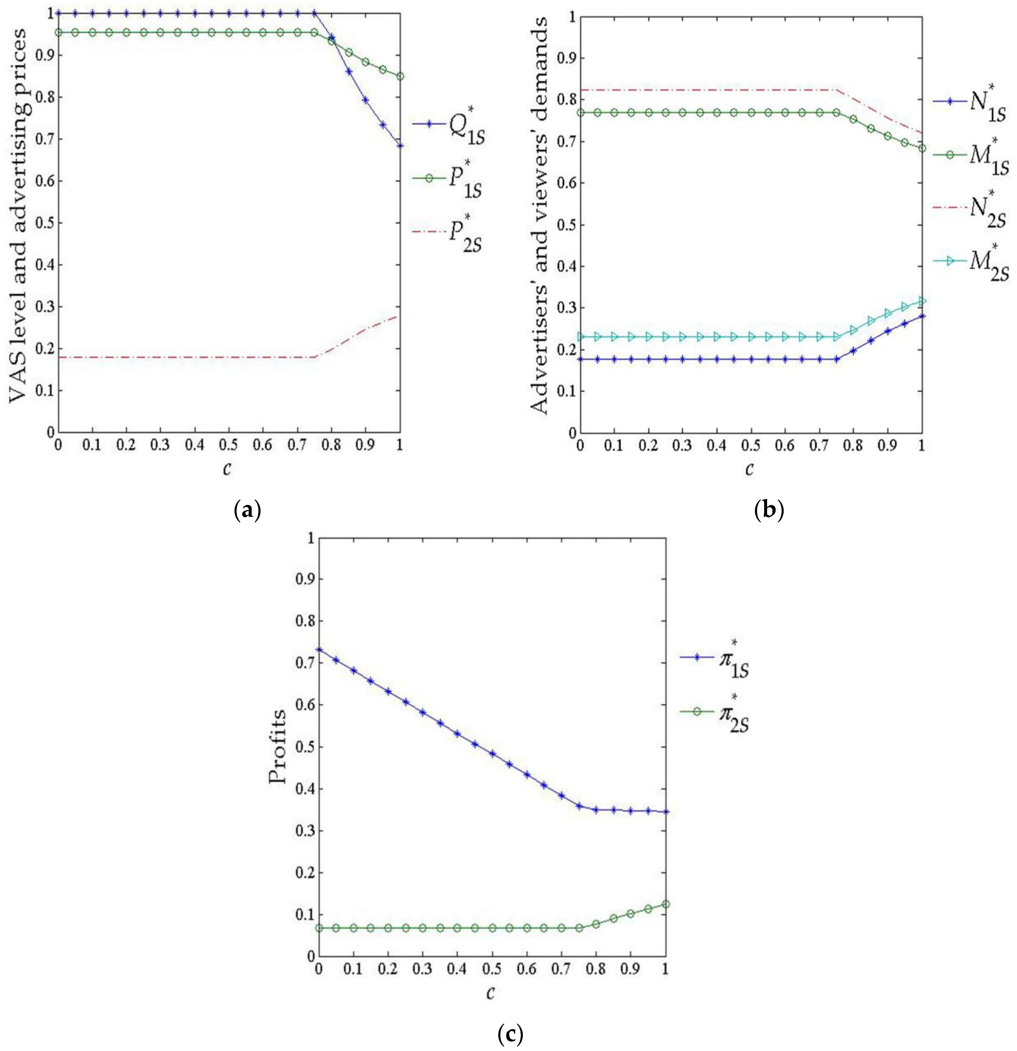
4.1. S-Model

For the S-Model, the viewers’ utility and advertisers’ utility from joining each platform and the two platforms’ profits are shown in

Table 1. Viewers’ utilities, advertisers’ utilities, and platforms’ profits in the S-Model.

Utility (or Profit)	Platform 1	Platform 2
Viewers’ utilities	$u_{1S}=V_{v0}-a{M}_{1S}-tx$	$u_{2S}=V_{v0}-a{M}_{2S}-t\left(1-x\right)$
Advertisers’ utilities	$U_{1S}=V_{a0}+r{N}_{1S}+Q_{1S}-P_{1S}-ty$	$U_{2S}=V_{a0}+r{N}_{2S}-P_{2S}-t\left(1-y\right)$
Platforms’ profits	${\pi }_{1S}=P_{1S}{M}_{1S}-c{\left(Q_{1S}\right)}^2/2$	${\pi }_{2S}=P_{2S}{M}_{2S}$

.

By solving $u_{1S}=u_{2S}$, we find that the marginal viewer who is indifferent as to which of the two platforms to join is located at

$$\overline{x}=\frac{t-M_{1S}a+M_{2S}a}{2t}.$$

All viewers to the left of $\overline{x}$ join platform 1 and all viewers to the right of $\overline{x}$ join platform 2.

Thus, viewers’ demand for platform 1, $N_{1S}$, and viewers’ demand for platform 2, $N_{2S}$, are given by

$$\{\begin{array}{c}{N}_{1S}=\frac{1}{2}+\frac{M_{2S}a-M_{1S}a}{2t},\\ N_{2S}=\frac{1}{2}-\frac{M_{2S}a-M_{1S}a}{2t}.\end{array}$$

(1)

Solving $U_{1S}=U_{2S}$, we find that the marginal advertiser who is indifferent as to which of the two platforms to join is located at

$$\overline{y}=\frac{1}{2}+\frac{P_{2S}-P_{1S}+Q_{1S}+N_{1S}r-N_{2S}r}{2t}.$$

Thus, advertisers’ demand for platform 1, $M_{1S}$, and advertisers’ demand for platform 2, $M_{2S}$, are given by

$$\{\begin{array}{c}{M}_{1S}=\frac{1}{2}+\frac{P_{2S}-P_{1S}+Q_{1S}+N_{1S}r-N_{2S}r}{2t},\\ M_{2S}=\frac{1}{2}-\frac{P_{2S}-P_{1S}+Q_{1S}+N_{1S}r-N_{2S}r}{2t}.\end{array}$$

(2)

Substituting $N_{1S}\mathrm{and}{N}_{2S}$ in Equation (1) into Equation (2), we can rewrite $M_{1S} \mathrm{and} M_{2S}$ as

$$\{\begin{array}{c}{M}_{1S}=\frac{1}{2}+\frac{P_{2S}t-P_{1S}t+t{Q}_{1S}-M_{1S}ar+M_{2S}ar}{2t^2},\\ M_{2S}=\frac{1}{2}-\frac{P_{2S}t-P_{1S}t+t{Q}_{1S}-M_{1S}ar+M_{2S}ar}{2t^2}.\end{array}$$

(3)

By $M_{1S}$ and $M_{2S}$ in Equation (3), we can further express $M_{1S} \mathrm{and} M_{2S}$ with respect to $P_{1S}$, $P_{2S}$ and $Q_{1S}$:

$$\{\begin{array}{c}{M}_{1S}=\frac{1}{2}+\frac{P_{2S}t-P_{1S}t+t{Q}_{1S}}{2\left(t^2+ar\right)},\\ M_{2S}=\frac{1}{2}+\frac{P_{1S}t-P_{2S}t-t{Q}_{1S}}{2\left(t^2+ar\right)}.\end{array}$$

(4)

Substituting $M_{1S}$ and $M_{2S}$ in Equation (4) into Equation (1), we obtain expressions for $N_{1S}$ and $N_{2S}$ with respect to $P_{1S}$, $P_{2S}$ and $Q_{1S}$:

$$\{\begin{array}{c}{N}_{1S}=\frac{1}{2}-\frac{a\left(P_{2S}-P_{1S}+Q_{1S}\right)}{2\left(t^2+ar\right)},\\ N_{2S}=\frac{a\left(P_{2S}-P_{1S}+Q_{1S}\right)}{2\left(t^2+ar\right)}+\frac{1}{2}.\end{array}$$

(5)

The profit-maximizing problems of platforms 1 and 2 can be written as follows:

$$\{\begin{array}{c}\max {\pi }_{1S}\left(P_{1S},Q_{1S}\right)=P_{1S}{M}_{1S}-\frac{c{\left(Q_{1S}\right)}^2}{2},\\ \max {\pi }_{2S}\left(P_{2S}\right)=P_{2S}{M}_{2S}.\end{array}$$

(6)

Substituting $M_{1S}$ and $M_{2S}$ in Equation (4) into Equation (6), we can rewrite the profit functions as follows:

$$\{\begin{array}{c}\max {\pi }_{1S}\left(P_{1S},Q_{1S}\right)=\frac{P_{1S}\left(ar-P_{1S}t+P_{2S}t+t{Q}_{1S}+t^2\right)}{2\left(t^2+ar\right)}-\frac{c{\left(Q_{1S}\right)}^2}{2},\\ \max {\pi }_{2S}\left(P_{2S}\right)=\frac{P_{2S}\left(ar+P_{1S}t-P_{2S}t-t{Q}_{1S}+t^2\right)}{2\left(t^2+ar\right)}.\end{array}$$

(7)

Solving Equation (7), we can obtain the optimal platform 1′s VAS level and advertising price, $Q_{1S}^{*}$ and $P_{1S}^{*}$, and platform 2′s advertising price $P_{2S}^{*}$, as given in Proposition 1. Furthermore, substituting $Q_{1S}^{*}$, $P_{1S}^{*}$ and $P_{2S}^{*}$ into Equations (4), (5), and (7), respectively, we derive the equilibrium advertisers’ and viewers’ demands for the two platforms and platforms’ profits, also as given in Proposition 1.

Proposition 1.

In the S-Model, in equilibrium, the VAS level, advertising prices, advertisers’ and viewers’ demands and profits are as follows:

• If $0\le c\le \left(3t^2+t+3ar\right)/6\left(t^2+ar\right)$,

  $$Q_{1S}^{*}=1,P_{1S}^{*}=\frac{3t^2+t+3ar}{3t},P_{2S}^{*}=\frac{3t^2-t+3ar}{3t},$$

  $$M_{1S}^{*}=\frac{3t^2+t+3ar}{6\left(t^2+ar\right)},M_{2S}^{*}=\frac{3t^2-t+3ar}{6\left(t^2+ar\right)},$$

  $$N_{1S}^{*}=\frac{3t^2-a+3ar}{6\left(t^2+ar\right)},N_{2S}^{*}=\frac{3t^2+a+3ar}{6\left(t^2+ar\right)},$$

  $${\pi }_{1S}^{*}=\frac{{\left(3t^2+t+3ar\right)}^2}{9t\left(2t^2+2ar\right)}-\frac{c}{2},{\pi }_{2S}^{*}=\frac{{\left(3t^2-t+3ar\right)}^2}{18t\left(t^2+ar\right)}.$$
• If $\left(3t^2+t+3ar\right)/6\left(t^2+ar\right)<c\le 1$,

  $$Q_{1S}^{*}=\frac{3\left(t^2+ar\right)}{6c{t}^2-t+6acr},P_{1S}^{*}=\frac{6\left(t^2+ar\right)\left(c{t}^2+acr\right)}{t\left(6c{t}^2-t+6acr\right)},P_{2S}=\frac{2\left(t^2+ar\right)\left(3c{t}^2-t+3acr\right)}{t\left(6c{t}^2-t+6acr\right)},$$

  $$M_{1S}^{*}=\frac{3c\left(t^2+ar\right)}{6c{t}^2-t+6acr},M_{2S}^{*}=\frac{3c{t}^2-t+3acr}{6c{t}^2-t+6acr},$$

  $$N_{1S}^{*}=\frac{6c{t}^2-t-a+6acr}{2\left(6c{t}^2-t+6acr\right)},N_{2S}^{*}=\frac{6c{t}^2-t+a+6acr}{2\left(6c{t}^2-t+6acr\right)},$$

  $${\pi }_{1S}^{*}=\frac{9c{\left(t^2+ar\right)}^2\left(4c{t}^2-t+4acr\right)}{2t{\left(6c{t}^2-t+6acr\right)}^2},{\pi }_{2S}^{*}=\frac{2\left(t^2+ar\right){\left(3c{t}^2-t+3acr\right)}^2}{t{\left(6c{t}^2-t+6acr\right)}^2}.$$

The proof of Proposition 1 can be found in Appendix A.

Based on Proposition 1, we analyze how marginal cost $c$ affects the equilibrium outcomes in the S-Model and obtain the following corollary.

Corollary 1.

In the S-Model, in equilibrium, the impacts of the marginal cost on the VAS level, advertising prices, as well as advertisers’ and viewers’ demands and profits are as follows:

• If $0\le c\le \left(3t^2+t+3ar\right)/6\left(t^2+ar\right)$,

  $$\frac{\partial Q_{1S}^{*}}{\partial c}=0,\frac{\partial P_{1S}^{*}}{\partial c}=0,\frac{\partial P_{2S}^{*}}{\partial c}=0.$$

  $$\frac{\partial M_{1S}^{*}}{\partial c}=0,\frac{\partial M_{2S}^{*}}{\partial c}=0,\frac{\partial N_{1S}^{*}}{\partial c}=0,\frac{\partial N_{2S}^{*}}{\partial c}=0,\frac{\partial {\pi }_{1S}^{*}}{\partial c}<0,\frac{\partial {\pi }_{2S}^{*}}{\partial c}=0.$$
• If $\left(3t^2+t+3ar\right)/6\left(t^2+ar\right)<c\le 1$,

  $$\frac{\partial Q_{1S}^{*}}{\partial c}<0,\frac{\partial P_{1S}^{*}}{\partial c}<0,\frac{\partial P_{2S}^{*}}{\partial c}>0,$$

  $$\frac{\partial M_{1S}^{*}}{\partial c}<0,\frac{\partial M_{2S}^{*}}{\partial c}>0,\frac{\partial N_{1S}^{*}}{\partial c}>0,\frac{\partial N_{2S}^{*}}{\partial c}<0,\frac{\partial {\pi }_{1S}^{*}}{\partial c}<0,\frac{\partial {\pi }_{2S}^{*}}{\partial c}>0.$$

The proof of Corollary 1 can be found in Appendix A.

If $0\le c\le \left(3t^2+t+3ar\right)/6\left(t^2+ar\right)$, the marginal cost that platform 1 invests in VASs for advertisers is relatively low. Thus, the VAS investment of platform 1 maintains the maximum, that is, $Q_{1S}^{*}=1$, indicating a higher (and constant) VAS benefit for advertisers. Within this range of $c$, as the marginal cost increases, the advertisers’ utility from joining platform 1 remains unchanged because of the constant VAS benefit. Likewise, the advertisers’ utility from joining platform 2, a platform without VASs, remains unchanged because advertisers receive no VAS benefit. This indicates that the advertisers’ demand for each platform remains unchanged; neither platform needs to adjust its advertising price. Indirectly, the viewers’ utility from joining platform $i$ ($i=1,2$) also remains unchanged within the range of $c$. This is because viewers, through the inter-group externality brought by advertisers, experience the same disutility from advertisers’ demand. Thus, the viewers’ demand for each platform also remains unchanged.

In addition, if the marginal cost is lower than $\left(3t^2+t+3ar\right)/6\left(t^2+ar\right)$, as the marginal cost increases, platform 1′s profit decreases with the marginal cost, while platform 2′s profit remains unchanged. The logic behind this result is as follows: For platform 1, although its advertising revenue is irrelevant to the marginal cost because of unchanged advertising price and advertisers’ demand, its investment cost increases with the marginal cost, which causes its profit to decrease with the marginal cost. For platform 2, its advertising revenue is irrelevant to the marginal cost and its investment cost is zero because it does not invest in VASs. Thus, its profit is not affected by the marginal cost.

If $\left(3t^2+t+3ar\right)/6\left(t^2+ar\right)<c\le 1$, the marginal cost that platform 1 invests in VASs for advertisers is relatively high. Thus, the VAS investment of platform 1 decreases with the marginal cost, which leads to a degree of utility loss for advertisers as well as a decrease in advertisers’ demand. To prevent further utility loss and a decrease in demand, platform 1 should lower its advertising price. However, the advertisers’ utility loss caused by reduced VASs is too great to be compensated for by lowered advertising price, ultimately leading certain advertisers to switch from platform 1 to platform 2. Hence, advertisers’ demand for platform 1 decreases and, in turn, their demand for platform 2 increases. Meanwhile, platform 2 charges a higher advertising price to obtain more profit. Due to a negative inter-group externality, advertisers’ decreased demand for platform 1 and increased demand for platform 2 leads to viewers’ increased demand for platform 1 and decreased demand for platform 2.

To further illustrate Corollary 1, a numerical analysis is performed. The parameters are set as $t=0.5$, $r=0.1$, and $a=0.6$. The impacts of marginal cost $c$ on VAS level, advertising prices, advertisers’ and viewers’ demands and profits are simulated and analyzed successively (Figure 2). As shown in Figure 2a–c, if $0\le c\le 0.769$, as the marginal cost increases, platform 1′s VAS level and advertising price, platform 2′s advertising price and profit, advertisers’ demands for the two platforms and viewers’ demands for the two platforms remain unchanged, while platform 1′s profit decreases. If $0.769<c\le 1$, as the marginal cost increases, platform 1′s VAS level, advertising price and profit decrease; platform 2′s advertising price and profit increase; advertisers’ demands for platform 1 and platform 2 decrease and increase, respectively; and viewers’ demand for platform 1 and platform 2 increase and decrease, respectively.

From Proposition 1, by comparing the equilibrium advertising prices and profits between platform 1 and platform 2 and comparing advertisers’ and viewers’ demands for platform 1 and for platform 2, we obtain Corollary 2.

Corollary 2.

In the S-Model, in equilibrium, the comparisons of the advertising prices and profits between the two platforms, the comparisons of advertisers’ demands for the two platforms and the comparisons of viewers’ demands for the two platforms are as follows:

$$P_{1S}^{*}>P_{2S}^{*},{\pi }_{1S}^{*}>{\pi }_{2S}^{*},M_{1S}^{*}>M_{2S}^{*},N_{1S}^{*}<N_{2S}^{*}.$$

The proof of Corollary 2 can be found in Appendix A.

Platform 1 can not only provide advertisers with a basic service such as that provided by platform 2 but can also provide a value-added service that is not provided by platform 2. Thus, advertisers’ utility and demand are improved on this platform. Advertisers’ increased demand for platform 1 leads to a decrease in viewers’ utility and demand on its platform through the negative inter-group network externality. In turn, this weakens the advertisers’ demand for platform 1 because of the positive inter-group network externality. In other words, the benefit of VAS investment is weakened because of the opposite inter-group network externalities between viewers and advertisers. Although the benefit is diminished, the advertisers’ utility and demand on platform 1 remain higher. Consequently, platform 1 sets a higher advertising price and achieves more advertising revenue. Platform 2′s lack of VASs means that advertisers obtain a lower gross utility from joining the platform; thus, the advertisers’ demand for platform 2 is lower. Thus, platform 2 sets a lower advertising price and obtains less advertising revenue. Furthermore, due to the negative inter-group network externality, the viewers’ demand is lower for platform 1 and higher for platform 2.

According to Corollary 2, platform 1′s profit is higher than platform 2′s. The intuitive reason for this result is straightforward; compared with platform 2, platform 1 can gain higher advertising revenue by providing VASs, while it also incurs a cost loss by investing in VASs. The increased advertising revenue is greater than this cost loss. Thus, platform 1 can obtain more profit than platform 2.

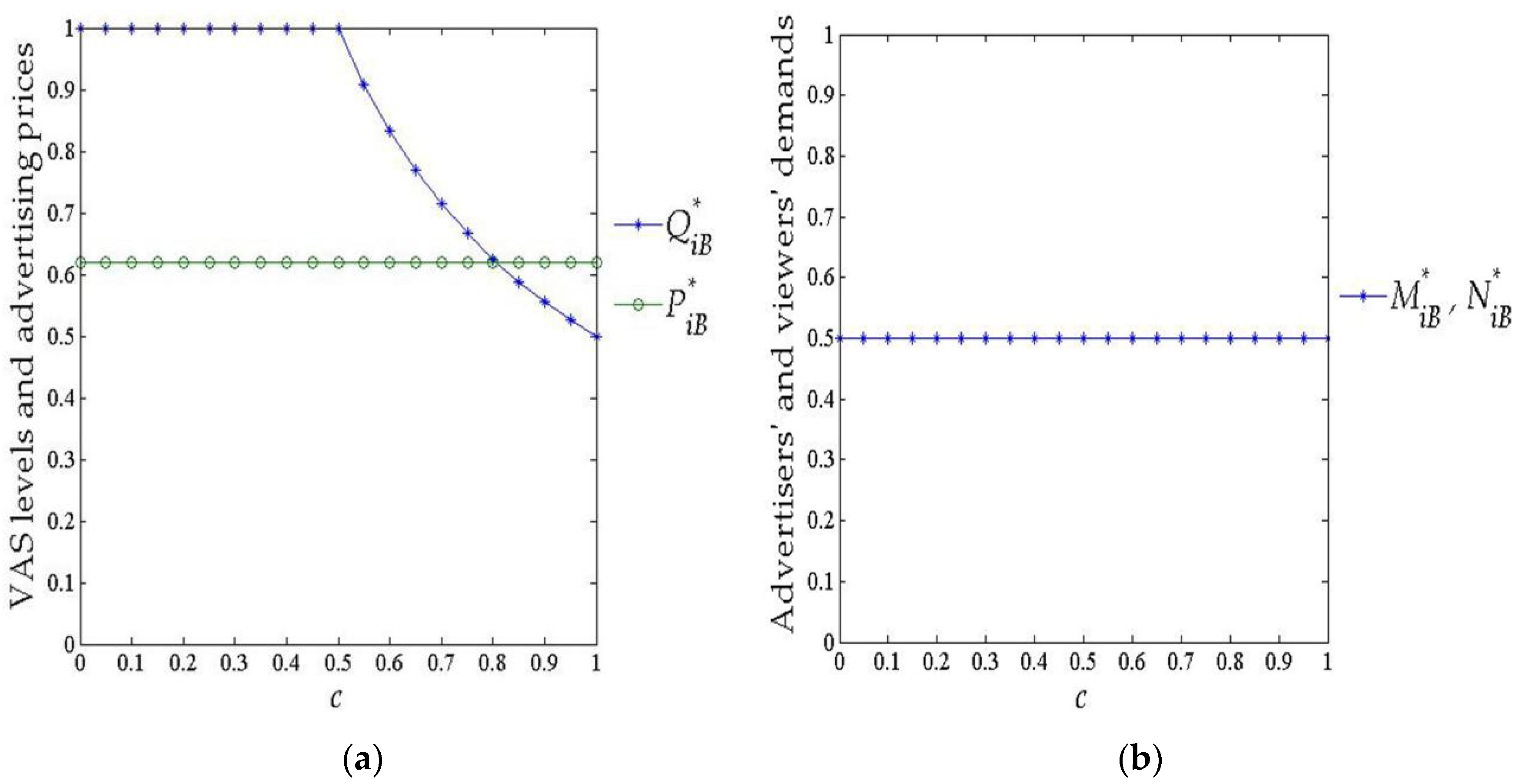
4.2. B-Model

As in Section 4.1, an equilibrium analysis of the B-Model was conducted.

For the B-Model, viewers’ utility and advertisers’ utility from joining each platform and the platforms’ profits are shown in

Table 2. Viewers’ utilities, advertisers’ utilities, and platforms’ profits in the B-Model.

Utility (or Profit)	Platform 1	Platform 2
Viewers’ utilities	$u_{1B}=V_{v0}-a{M}_{1B}-tx$	$u_{2B}=V_{v0}-a{M}_{2B}-t\left(1-x\right)$
Advertisers’utilities	$U_{1B}=V_{a0}+r{N}_{1B}+Q_{1B}-P_{1B}-ty$	$U_{2B}=V_{a0}+r{N}_{2B}+Q_{2B}-P_{2B}-t\left(1-y\right)$
Platforms’profits	${\pi }_{1B}=P_{1B}{M}_{1B}-c{\left(Q_{1B}\right)}^2/2$	${\pi }_{2B}=P_{2B}{M}_{2B}-c{\left(Q_{2B}\right)}^2/2$

.

In an approach similar to the one adopted for the S-Model, we can express advertisers’ and viewers’ demands as functions of the VAS levels and prices in the B-Model, as given by

$$\{\begin{array}{c}{M}_{1B}=\frac{1}{2}-\frac{t\left(P_{1B}-P_{2B}-Q_{1B}+Q_{2B}\right)}{2\left(t^2+ar\right)},\\ M_{2B}=\frac{1}{2}+\frac{t\left(P_{1B}-P_{2B}-Q_{1B}+Q_{2B}\right)}{2\left(t^2+ar\right)}.\end{array}$$

(8)

$$\{\begin{array}{c}{N}_{1B}=\frac{a\left(P_{1B}-P_{2B}-Q_{1B}+Q_{2B}\right)}{2\left(t^2+ar\right)}+\frac{1}{2},\\ N_{2B}=\frac{1}{2}-\frac{a\left(P_{1B}-P_{2B}-Q_{1B}+Q_{2B}\right)}{2\left(t^2+ar\right)}.\end{array}$$

(9)

The maximization problems of the two platforms can be given as follows:

$$\{\begin{array}{c}max{\pi }_{1B}\left(P_{1B},Q_{1B}\right)=P_{1B}{M}_{1B}-\frac{c{\left(Q_{1B}\right)}^2}{2},\\ max{\pi }_{2B}\left(P_{2B},Q_{2B}\right)=P_{2B}{M}_{2B}-\frac{c{\left(Q_{2B}\right)}^2}{2}.\end{array}$$

(10)

Substituting $M_{1B}$ and $M_{2B}$ in Equation (8) into Equation (10), we can rewrite the profit functions (10) as follows:

$$\{\begin{array}{c}max{\pi }_{1B}\left(P_{1B},Q_{1B}\right)=\frac{P_{1B}\left(ar-P_{1B}t+P_{2B}t+t{Q}_{1B}-t{Q}_{2B}+t^2\right)}{2\left(t^2+ar\right)}-\frac{c{\left(Q_{1B}\right)}^2}{2},\\ max{\pi }_{2B}\left(P_{2B},Q_{2B}\right)=\frac{P_{2B}\left(ar+P_{1B}t-P_{2B}t-t{Q}_{1B}+t{Q}_{2B}+t^2\right)}{2\left(t^2+ar\right)}-\frac{c{\left(Q_{2B}\right)}^2}{2}.\end{array}$$

(11)

Solving Equation (11), we can obtain the optimal VAS levels and advertising prices, $Q_{iB}^{*}$ and $P_{iB}^{*}$, $i=1,2$, as given in Proposition 2. Furthermore, substituting $Q_{iB}^{*}$ and $P_{iB}^{*}$ into Equations (8)–(10), respectively, we derive the equilibrium advertisers’ and viewers’ demands, $M_{iB}^{*}$ and $N_{iB}^{*}$, and platforms’ profits, ${\pi }_{iB}^{*}$, also as given in Proposition 2.

Proposition 2.

In the B-Model, in equilibrium, the VAS levels, advertising prices, advertisers’ and viewers’ demands and profits are as follows:

• If $0\le c\le 1/2$,

  $$Q_{iB}^{*}=1,P_{iB}^{*}=\frac{t^2+ar}{t},M_{iB}^{*}=\frac{1}{2},N_{iB}^{*}=\frac{1}{2},{\pi }_{iB}^{*}=\frac{t^2-ct+ar}{2t}.$$
• If $1/2<c\le 1$,

  $$Q_{iB}^{*}=\frac{1}{2c},P_{iB}^{*}=\frac{t^2+ar}{t},M_{iB}^{*}=\frac{1}{2},N_{iB}^{*}=\frac{1}{2},{\pi }_{iB}^{*}=\frac{4c{t}^2-t+4acr}{8ct}.$$

The proof of Proposition 2 can be found in Appendix A.

Based on Proposition 2, we investigate the impact of marginal cost $c$ on the equilibrium outcomes in the B-Model and obtain Corollary 3.

Corollary 3.

In the B-Model, in equilibrium, the impacts of the marginal cost on the VAS levels, advertising prices, advertisers’ and viewers’ demands and profits are as follows:

• If $0\le c\le 1/2$,

  $$\frac{\partial Q_{iB}^{*}}{\partial c}=0,\frac{\partial P_{iB}^{*}}{\partial c}=0,\frac{\partial M_{iB}^{*}}{\partial c}=0,\frac{\partial N_{iB}^{*}}{\partial c}=0,\frac{\partial {\pi }_{iB}^{*}}{\partial c}<0.$$
• If $1/2<c\le 1$,

  $$\frac{\partial Q_{iB}^{*}}{\partial c}<0,\frac{\partial P_{iB}^{*}}{\partial c}=0,\frac{\partial M_{iB}^{*}}{\partial c}=0,\frac{\partial N_{iB}^{*}}{\partial c}=0,\frac{\partial {\pi }_{iB}^{*}}{\partial c}>0.$$

The proof of Corollary 3 can be found in Appendix A.

If $0\le c\le 1/2$, investing in a unit of VAS level costs little, both platforms are willing to maintain the maximum VAS levels, that is, $Q_{1B}^{*}=1,Q_{2B}^{*}=1$. With the fixed VAS level, the benefit that advertisers derive from VASs on each platform remains unchanged, implying that advertisers’ utility and demand on each platform likewise remain unchanged. Consequently, neither platform needs to adjust its advertising price. As a result, within this range of $c$, for each platform, its advertising revenue remains the same. Overall investment cost increases with the marginal cost and this results in its profit decreasing with the cost. If $1/2<c\le 1$, investing in a unit of VAS level costs more, so both platforms reduce their VAS levels as the marginal cost increases, leading to a reduction in advertisers’ utility on both platforms. A symmetric reduction in VASs on both platforms means that advertisers’ utility losses are the same on both platforms. As a result, advertisers’ gross utility from either platform is the same, implying that each platform accounts for half of the total advertisers’ demand. Indirectly, due to the inter-group network externality brought by advertisers, viewers’ utility is the same from joining either platform, so each platform accounts for half of the total viewers’ demand. Obviously, for both advertisers and viewers, the demand for either platform is independent of the marginal cost. Note that Corollary 3 shows that each platform’s profit increases with the marginal cost if $1/2<c\le 1$. The intuitive reason for this result is straightforward; for each platform, the advertising revenue is irrelevant to the marginal cost. However, the overall investment cost decreases sharply with the marginal cost, leading to increased profit with increased marginal cost.

To further reflect Corollary 3, a numerical analysis is performed. The parameters are set to $t=0.5$, $r=0.1$ and $a=0.6$. The impacts of marginal cost $c$ on VAS levels, advertising prices, advertisers’ and viewers’ demands and profits are simulated and analyzed (Figure 3). Based on Figure 3, we can derive that, if $0\le c\le 0.5$, as the marginal cost increases, the two platforms’ VAS levels and advertising prices, advertisers’ demands for the two platforms and viewers’ demands for the two platforms remain unchanged and the two platforms’ profits decrease. If $0.5<c\le 1$, as the marginal cost increases, the two platforms’ VAS levels decrease, the advertising prices and advertisers’ and viewers’ demands for the two platforms remain unchanged and the two platforms’ profits increase.

5. Comparison of the Equilibrium Outcomes

Based on the equilibrium outcomes in Section 4, we first compare platforms’ VAS levels and advertising prices between the two scenarios with VAS investment, i.e., the S-Model and B-Model. Then, we compare platforms’ advertising prices between each scenario with VAS investment and the scenario without VAS investment, i.e., we compare the S-Model with the scenario without VAS investment, as well as the B-Model with the scenario without VAS investment.

5.1. S-Model vs. B-Model

This subsection compares platforms’ VAS levels and advertising prices between the S-Model and B-Model, the two scenarios with VAS investment. Since platform 2 does not develop VASs for advertisers in the S-Model, it is not meaningful to compare platform 2′s VAS levels between the models. Thus, in this section, we compare only platform 1′s VAS levels between the models.

Based on the equilibrium outcomes described in Proposition 1 and Proposition 2, comparing platform 1′s VAS levels and the two platforms’ advertising prices between the S-Model and B-Model, we obtain Corollary 4.

Corollary 4.

The comparisons of platform 1′s VAS levels and the two platforms’ advertising prices between the S-Model and B-Model are as follows:

• If $0\le c\le 1/2$, $Q_{1S}^{*}=Q_{1B}^{*}$; if $1/2<c\le 1$, $Q_{1S}^{*}>Q_{1B}^{*}$.
• For $\forall c\in \left[0,1\right]$, $P_{1S}^{*}>P_{1B}^{*}$, $P_{2S}^{*}<P_{2B}^{*}$.

The proof of Corollary 4 can be found in Appendix A.

If $0\le c\le 1/2$, investing in a unit of VAS level costs less and platform 1 is willing to maintain the maximum VAS level in both the S-Model and B-Model, that is, $Q_{1B}^{*}=1$ and $Q_{1S}^{*}=1$. If $1/2<c\le 1$, investing in a unit of VAS level costs more; platform 1 has a weak incentive to invest in VASs—lower in the B-Model than in the S-Model. The reason is as follows. In the S-Model, platform 1 invests in VASs exclusively. Thus, compared to platform 2, platform 1 offers advertisers additional benefits. More advertisers join platform 1 and the platform accounts for more than half of the total advertisers’ demand. Accordingly, platform 1 can set a higher advertising price and obtain more advertising revenue by taking advantage of such conditions. However, in the B-Model, symmetric VAS levels in platforms 1 and 2 lead to the same advertisers’ gross utility from either platform; each platform accounts for half of the total advertisers’ demand. Because platform 1, providing the same VASs as platform 2, has no competitive advantages, it cannot set the higher price that is available in the S-Model; hence, platform 1 obtains less advertising revenue. Based on the preceding analysis, platform 1 can obtain more revenue by investing in VASs in the S-Model than the B-Model; therefore, it has a greater motivation to invest in VASs in the S-Model.

Corollary 4 shows that, for $\forall c\in \left[0,1\right]$, platform 2′s advertising price is lower in the S-Model than in the B-Model. The intuitive explanation for this is straightforward; in the S-Model, because platform 2 does not invest in VASs, advertisers lose a degree of utility. Therefore, to avoid excessive utility loss for advertisers, platform 2 can only set a lower advertising price.

5.2. S-Model vs. the Scenario without VAS Investment

Since neither platform develops VASs in the scenario without VAS investment, it is not meaningful to compare the two platforms’ VAS levels between the S-Model and the scenario without VAS investment. This subsection compares only platforms’ advertising prices between the S-Model and the scenario without VAS investment.

Prior to the comparison, we briefly analyze the equilibrium outcomes in the scenario without VAS investment (see Appendix A) and obtain the following equilibrium outcomes:

$$P_{iW}^{*}=\frac{t^2+ar}{t},M_{iW}^{*}=\frac{1}{2},N_{iW}^{*}=\frac{1}{2},{\pi }_{iW}^{*}=\frac{t^2+ar}{2t},i=1,2.$$

By comparing platform $i$’s advertising prices between the S-Model and the scenario without VAS investment, we obtain Corollary 5.

Corollary 5.

The comparisons of the two platforms’ advertising prices between the S-Model and the scenario without VAS investment are as follows: $P_{1S}^{*}>P_{1W}^{*}$and$P_{2S}^{*}<P_{2W}^{*}$.

The proof of Corollary 5 can be found in Appendix A.

The intuitive reason for platform 1′s higher advertising price in the S-Model than in the scenario without VAS investment is as follows. In the S-Model, the additional benefit from platform 1′s exclusive VASs improves advertisers’ utility and platform 1 charges a higher advertising price to obtain more revenue. However, in the scenario without VAS investment, neither platform can provide VASs; thus, advertisers cannot gain an additional utility by selecting platform 1 over platform 2. Consequently, platform 1 cannot set a higher advertising price as it is able to do in the S-Model.

Corollary 5 also indicates that platform 2′s advertising price is lower in the S-Model than in the scenario without VAS investment. The reason for this is as follows. In the S-Model, due to the unavailability of VASs, advertisers lose utility by joining platform 2 instead of platform 1. Therefore, to avoid excessive utility loss for advertisers, platform 2 lowers its advertising price. However, in the scenario without VAS investment, advertisers cannot benefit from VASs from any platform, which indicates that advertisers do not lose more utility by joining platform 2 instead of platform 1. In this scenario, platform 2 does not need to lower its advertising price to avoid utility loss.

5.3. B-Model vs. the Scenario without VAS Investment

By comparing the two platforms’ advertising prices between the B-Model and the scenario without VAS investment, we obtain Corollary 6.

Corollary 6.

The comparisons of the two platforms’ advertising prices between the B-Model and the scenario without VAS investment are as follows: $P_{iB}^{*}=P_{iW}^{*}$, $i=1,2$.

The proof of Corollary 6 can be found in Appendix A.

Corollary 6 shows that each platform’s advertising price in the B-Model is the same as in the scenario without VAS investment.

6. Conclusions

This paper investigates duopolistic video platforms’ VAS investment strategies and pricing strategies for advertisers. We consider two scenarios with VAS investment for advertisers, i.e., an asymmetric investment scenario and a symmetric investment scenario, denoted by the S-Model and the B-Model, respectively. In each model, the optimal VAS levels and advertising prices can be obtained by an equilibrium analysis. Then, we compare the optimal VAS levels and advertising prices between the S-Model and B-Model. We also compare the advertising prices between each scenario with VAS investment and the scenario without VAS investment, i.e., we compare S-Model with the scenario without VAS investment, as well as the B-Model with the scenario without VAS investment.

The main findings are offered. (i) In the S-Model, for the investing platform, if the marginal cost is low, its VAS level maintains the maximum, and its advertising price is independent of the marginal cost; otherwise, its VAS level and advertising price decrease with the marginal cost. For the non-investing platform, if the marginal cost is low, its advertising price is independent of the marginal cost; otherwise, its advertising price increases with the marginal cost. Comparatively, the investing platform’s advertising price is higher than the non-investing platform’s. (ii) In the B-Model, for each platform, if the marginal cost is low, its VAS level maintains the maximum, and its advertising price is independent of the marginal cost; otherwise, its VAS level decreases with the marginal cost and its advertising price is also independent of the marginal cost. In addition, the two platforms’ VAS levels and advertising prices are equal. (iii) The investing platform’s VAS level in the S-Model is higher than or the same as that in the B-Model and the investing platform’s advertising price in the S-Model is higher than that in the B-Model. (iv) Compared to the scenario without VAS investment, the investing platform’s advertising price is higher in the S-Model, while it is the same in the B-Model.

This study contributes to the literature on media platforms’ pricing strategies by analyzing such pricing strategies by considering the platforms’ VAS investments for advertisers. To the best of my knowledge, previous literature on media platforms’ pricing strategies has predominantly focused on the factors that affect them, such as the differentiation level between platforms, advertising charge models, etc. However, previous studies have not focused on the impact of platforms’ VAS investment on such pricing strategies. We suppose this study is the first step in exploring media platforms’ pricing strategies under the impact of platforms’ VAS investment. This study argues that, when a single platform invests in VASs for advertisers, whether the two platforms’ advertising prices are affected by the marginal cost of investing in VASs depends on the value of the marginal cost. When both platforms invest in VASs for advertisers, the two platforms’ advertising prices are independent of the marginal cost. This study also finds that the investing platform’s advertising price is higher when a single platform invests in VASs for advertisers than when both platforms invest in VASs for advertisers.

This study adds to the literature on platforms’ VAS investment strategies by examining the VAS investment strategies of idiosyncratic platforms, i.e., media platforms, in a duopoly setting. This study finds that, if the marginal investing cost is low, the investing platform should exhaust all resources to invest in VASs; otherwise, as the marginal cost increases, the platform should reduce its investment in VASs. This conclusion is supported by Dou and He [27], who investigated the VAS investments and pricing strategies of general platforms in a monopoly setting. In addition, this paper shows that if the marginal investing cost is low, the platform’s price to invested users is not affected by the marginal cost, which is consistent with Dou et al. [26]. However, different from Dou et al. [26], this study reveals that, if the marginal cost is high, the platform’s price to invested users may not necessarily decrease with the marginal cost, whether it decreases or not, depending on the symmetry of VAS investment. Specifically, in an asymmetric investment scenario, the price decreases with the marginal cost, while, in a symmetric investment scenario, the price is independent of the marginal cost. Moreover, this study reveals that compared to the scenario without VAS investment, the platform’s price to invested users may not necessarily be higher in the scenario with VAS investment, which is also different from Dou et al. [26]. Specifically, in an asymmetric investment scenario, the platform’s price for invested users is higher in the scenario with VAS investment than in the scenario without VAS investment; however, in a symmetric investment scenario, the prices in scenarios with VAS investment and without VAS investment are equal.

COVID-19 pandemic has dramatically changed the world, not only in terms of public health, but also in terms of access to information and entertainment. During the COVID-19 pandemic, more and more people have turned to online video platforms for their entertainment needs, which provides favorable opportunities for the development of video platforms. Since most video platforms derive their main revenue from advertising, they need to formulate appropriate VAS investment strategies and pricing strategies for advertisers to ensure sustainable development. The findings of this study have important management implications for video platforms in making operational decisions on VAS levels and advertising prices. (i) A video platform should consider the impact of the marginal VAS investing cost when it determines the VAS level it should invest in for advertisers. Regardless of whether its competitor invests in VASs, a video platform should maintain the maximum VAS level if the marginal VAS investing cost is low and should appropriately reduce the VAS level as the marginal VAS investing cost increases if the marginal VAS investing cost is high. In reality, the VASs provided by the platform to advertisers involve the processing of viewers’ personal data. For example, the platform processes viewers’ information to assist advertisers with improving their decision-making. During this processing, the video platform should comply with Article 32 of General Data Protection Regulation (GDPR) [33]; thus, the platform needs to implement appropriate technical measures to ensure a certain level of security to prevent viewers’ personal data from being at risk. For example, pseudonymization technology and encryption technology are used in data processing [33]. The implementation of these technical measures will cause the platform to incur a cost, which is part of the VAS investing cost mentioned in this paper. If the marginal VAS investing cost is low due to a low marginal cost of implementing these technical measures, we suggest that the investing platform should maintain the maximum VAS level. And if the marginal VAS investing cost is high due to a high marginal cost of implementing these technical measures, we suggest that the platform should reduce the VAS level as the marginal VAS investing cost increases. (ii) The platform should effectively coordinate its advertising pricing strategy with the VAS investment strategy when it invests in VASs for advertisers. If the platform is the exclusive investor, it should maintain a constant advertising price when the marginal VAS investing cost is low and it should appropriately lower the advertising price as the marginal VAS investing cost increases when the marginal VAS investing cost is high. If the platform is a non-exclusive investor, i.e., the platform’s competitor also invests in VASs, it should maintain a constant advertising price, regardless of whether the marginal VAS investing cost is high or low.

This study has two main limitations that suggest future research directions. First, we assume, in this paper, that viewers are single-homing. However, in reality, viewers may be multi-homing. Thus, it is meaningful to consider a setting in which viewers are multi-homing. Second, we only consider the inter-group network externalities between the viewers and the advertisers, while ignoring the intra-group network externality among the advertisers. It would be interesting to explore media platforms’ optimal VAS investment and pricing strategies while considering the advertisers’ intra-group network externality.

References

- Yang, Z.; Diao, Z.; Kang, J. Customer management in Internet-based platform firms: Review and future research directions. Mark. Intell. Plan. 2020, 38, 957–973. [Google Scholar] [CrossRef]
- Jullien, B.; Sand-Zantman, W. The economics of platforms: A theory guide for competition policy. Inf. Econ. Policy 2021, 54, 100880. [Google Scholar] [CrossRef]
- Xie, J.; Zhu, W.; Wei, L.; Liang, L. Platform competition with partial multi-homing: When both same-side and cross-side network effects exist. Int. J. Prod. Econ. 2021, 233, 108016. [Google Scholar] [CrossRef]
- Ge, J.; Li, T. Entrepreneurial resources, complementary assets, and platform sustainability. Sustainability 2019, 11, 4359. [Google Scholar] [CrossRef] [Green Version]
- Amaldoss, W.; Du, J.; Shin, W. Media platforms’ content provision strategies and sources of profits. Mark. Sci. 2021, 40, 527–547. [Google Scholar] [CrossRef]
- Lin, Z. Commercialization of creative videos in China in the digital platform age. Telev. New Media 2020, 21, 1527476420953583. [Google Scholar] [CrossRef]
- Xu, S.; Ling, L. Which is the optimal commercial mode for a video site: Paid, free, or hybrid? Asia Pac. J. Oper. Res. 2020, 37, 2050022. [Google Scholar] [CrossRef]
- Kodera, T. Discriminatory pricing and spatial competition in two-sided media markets. BE J. Econ. Anal. Policy 2015, 15, 891–926. [Google Scholar] [CrossRef]
- Zennyo, Y. Freemium competition among ad-sponsored platforms. Inf. Econ. Policy 2020, 50, 100848. [Google Scholar] [CrossRef]
- Annual and Transition Report of Foreign Private Issuers. Available online: https://www.sec.gov/ix?doc=/Archives/edgar/data/0001722608/000156459021011590/iq-20f_20201231.htm (accessed on 31 December 2020).
- Sato, S. Freemium as optimal menu pricing. Int. J. Ind. Organ. 2019, 63, 480–510. [Google Scholar] [CrossRef] [Green Version]
- Liu, H.; Liu, S. Considering in-app advertising mode, platform-app channel coordination by a sustainable cooperative advertising mechanism. Sustainability 2020, 12, 145. [Google Scholar] [CrossRef] [Green Version]
- Reisinger, M. Platform competition for advertisers and users in media markets. Int. J. Ind. Organ. 2012, 30, 243–252. [Google Scholar] [CrossRef]
- Dietl, H.; Lang, M.; Lin, P. Advertising pricing models in media markets: Lump-sum versus per-consumer charges. Inf. Econ. Policy 2013, 25, 257–271. [Google Scholar] [CrossRef] [Green Version]
- Pan, L. Endogenous choice on advertising pricing of media platforms: Lump-sum fee vs. proportional fee. Hitotsubashi J. Econ. 2017, 58, 21–40. [Google Scholar] [CrossRef] [Green Version]
- Pan, L. Pricing of media platforms with vertical differentiation. Econ. Comput. Econ. Cybern. Stud. 2017, 51, 249–262. [Google Scholar]
- Chen, M.; Rennhoff, A.D.; Serfes, K. Bundling, à la carte pricing and vertical bargaining in a two-sided model. Inf. Econ. Policy 2016, 35, 30–44. [Google Scholar] [CrossRef]
- Greiner, T.; Sahm, M. How effective are advertising bans? On the demand for quality in two-sided media markets. Inf. Econ. Policy 2018, 43, 48–60. [Google Scholar] [CrossRef] [Green Version]
- Anderson, S.P.; Foros, Ø.; Kind, H.J. Competition for advertisers and for viewers in media markets. Econ. J. 2018, 128, 34–54. [Google Scholar] [CrossRef]
- Carronia, E.; Dimitri, P. Business models for streaming platforms: Content acquisition, advertising and users. Inf. Econ. Policy 2020, 52, 100877. [Google Scholar] [CrossRef]
- Park, K.F.; Seamans, R.; Zhu, F. Homing and platform responses to entry: Historical evidence from the U.S. newspaper industry. Strateg. Manag. J. 2021, 42, 684–709. [Google Scholar] [CrossRef]
- Hagiu, A.; Spulber, D. First-party content and coordination in two-sided markets. Manag. Sci. 2013, 59, 933–949. [Google Scholar] [CrossRef]
- Anderson Jr, E.G.; Parker, G.G.; Tan, B. Platform performance investment in the presence of network externalities. Inf. Syst. Res. 2014, 25, 152–172. [Google Scholar] [CrossRef]
- Tan, B.; Anderson Jr, E.G.; Parker, G. Platform pricing and investment to drive third party value creation in two-sided networks. Inf. Syst. Res. 2020, 31, 217–239. [Google Scholar] [CrossRef] [Green Version]
- Lin, X.; Chen, C.; Lin, Z.; Zhou, Y. Pricing and service strategies for two-sided platforms. J. Syst. Sci. Syst. Eng. 2019, 28, 299–316. [Google Scholar] [CrossRef]
- Dou, G.; He, P.; Xu, X. One-side value-added service investment and pricing strategies for a two-sided platform. Int. J. Prod. Res. 2016, 54, 3808–3821. [Google Scholar] [CrossRef]
- Dou, G.; He, P. Value-added service investing and pricing strategies for a two-sided platform under investing resource constraint. J. Syst. Sci. Syst. Eng. 2017, 26, 609–627. [Google Scholar] [CrossRef]
- Dou, G.; Lin, X.; Xu, X. Value-added service investment strategy of a two-sided platform with the negative intra-group network externality. Kybernetes 2018, 47, 937–956. [Google Scholar] [CrossRef]
- Kim, Y.; Mo, J. Pricing of digital video supply chain: Free versus paid service on the direct distribution channel. Sustainability 2019, 11, 46. [Google Scholar] [CrossRef] [Green Version]
- Calvano, E.; Polo, M. Market power, competition and innovation in digital markets: A survey. Inf. Econ. Policy 2021, 54, 100853. [Google Scholar] [CrossRef]
- D’Annunzio, A.; Russo, A. Ad networks and consumer tracking. Manag. Sci. 2020, 66, 5040–5058. [Google Scholar] [CrossRef] [Green Version]
- Dindaroglu, B. Competitive advertising on broadcasting channels and consumer welfare. Inf. Econ. Policy 2018, 42, 66–75. [Google Scholar] [CrossRef]
- General Data Protection Regulation. Available online: https://gdpr-info.eu/ (accessed on 25 May 2018).