Abstract
Integration of Distributed generations (DGs) and capacitor banks (CBs) in distribution systems (DS) have the potential to enhance the system’s overall capabilities. This work demonstrates the application of a hybrid optimization technique the applies an available renewable energy potential (AREP)-based, hybrid-enhanced grey wolf optimizer–particle swarm optimization (AREP-EGWO-PSO) algorithm for the optimum location and sizing of DGs and CBs. EGWO is a metaheuristic optimization technique stimulated by grey wolves, and PSO is a swarm-based metaheuristic optimization algorithm. Hybridization of both algorithms finds the optimal solution to a problem through the movement of the particles. Using this hybrid method, multi-criterion solutions are obtained, such as technical, economic, and environmental, and these are enriched using multi-objective functions (MOF), namely minimizing active power losses, voltage deviation, the total cost of electrical energy, total emissions from generation sources and enhancing the voltage stability index (VSI). Five different operational cases were adapted to validate the efficacy of the proposed scheme and were performed on two standard distribution systems, namely, IEEE 33- and 69-bus radial distribution systems (RDSs). Notably, the proposed AREP-EGWO-PSO algorithm compared the AREP at the candidate locations and re-allocated the DGs with optimal re-sizing when the EGWO-PSO algorithm failed to meet the AREP constraints. Further, the simulated results were compared with existing optimization algorithms considered in recent studies. The obtained results and analysis show that the proposed AREP-EGWO-PSO re-allocates the DGs effectively and optimally, and that these objective functions offer better results, almost similar to EGWO-PSO results, but more significant than other existing optimization techniques.
1. Introduction
Distributed generations (DGs) have become an attractive option for integrating power distribution systems due to their economic, technical, and environmental advantages [1,2]. Although DGs can offer several benefits to the system, their installation is subject to their primary energy source’s availability and geographical location [3]. On the other hand, DGs can cause undesired effects in the system, such as fluctuations in the voltage profile, increased fault current, and inversion in the power flow direction, etc. [4,5]. These effects become more evident when DGs use renewable energy resources (RER). RER play an energetic role in resolving environmental and security issues. They have a probabilistic nature, such as wind speed and solar irradiation [6]. Therefore, technical studies should be conducted to properly install DGs in passive systems, avoiding the degradation of reliability, system operation, and supply quality [3].
In a radial distribution system (RDS), the reactive power flow is considered the main reason for power quality issues [6]. The compensation of reactive power plays the leading part in power system planning. The capacitor banks (CBs) are treated as the familiar reactive power resources that offer loss reduction, voltage regulation, stability improvement, and a financial return for distribution companies when optimally installed in distribution systems [3,7,8].
To reduce the overall production costs and improve system reliability, both the DGs and CBs are commissioned as real and reactive power injection sources [7]. The installation of DG and the capacitor in the distribution network has various technical and economic benefits [9]. These multiple benefits cannot be achieved without the appropriate allocation of the DGs and CBs in power system networks. Further, the optimal allocation of both DG and CB can be carried out using optimization techniques using several methodologies [10]. The complete analysis of the existing works relating to the optimization is described in the following section.
The techniques proposed for the placement of DG and CB in distribution networks can be divided into four types: numerical, analytical, metaheuristic, and hybrid optimization [10,11]. The analytical methods have fast convergence, but their computational time and complexity become high when the type and number of DGs and CBs increases [12]. This is particularly true for multi-objective formulations with a large number of equality and inequality constraints. Analytical approaches require more robust algorithms to solve differential and nonlinear equations. In this respect, metaheuristic techniques are helpful in solving the distribution system problems which do not involve differential equations. However, the algorithms need to be appropriately tuned to reach the global solution for DG sizing and placement [12,13].
Among various metaheuristic optimization techniques, particle swarm optimization (PSO) is the most widely used for the siting and sizing DGs. PSO has significantly better computation efficiency, i.e., its functional evaluation. A vital issue with PSO is the trapping of particles into local optima that could consume a large amount of time to converge to an optimal solution. Additionally, there is no guarantee that the optimal solution will be global optima. As a result, several research works highlighted the hybridization of the standard PSO with analytical approaches or other optimization techniques for achieving better results [14]. By using a hybrid optimization technique, better optimization results can be produced by merging two optimization algorithms [9]. Instead of searching in the whole area, the search space is limited by loss sensitivity factor (LSF), increasing the possibility of finding a good solution. After selecting the candidate buses by LSF, an optimizer finds the optimum size of DGs and CBs on the buses. Consequently, a fast convergence is achieved without compromising the siting and sizing aspects [10,14].
2. Literature Surveys
A complete survey of numerous literary works associated with the optimal installation of DGs and CBs is elaborated in Table 1 [15,16].

Table 1.
Survey of prevailing research works with respect to optimal installation of DGs and CBs.
The existing works demonstrate the optimal allocation of DGs without considering the potential of the renewable resources. Further, optimal DG allocation combined with the potential assessment of renewable energy sources (RESs) could save time, effort, and planning for current and future DG unit installations [28] for real-time systems. This work examines the available renewable energy potentials (AREPs) at all the locations of IEEE 33- and 69-bus RDSs. The renewable energy technologies in this study include solar photovoltaic (PV), wind turbine (WT), and gas turbine (GT).
A summary of the limitations of existing works is as follows:
- DGs with unity power factor (UPF) alone has been considered in few approaches.
- In a few cases, CBs and/or DGs locations were fixed.
- Economic and environmental implications and a few network constraints have been ignored.
- The simulation time and the results have been non-optimal in few existing techniques.
- Re-allocation of DGs based on available renewable energy potential (AREP) has not been considered.
Based on these limitations, the distribution network performance needs to be improved further using DGs in accordance with AREP. Therefore, a new multi-objective AREP-based hybrid optimization technique is proposed by combining enhanced grey wolf optimizer with particle swarm optimization (AREP-EGWO-PSO). This hybridization can incorporate the benefits of both methods and overcome the drawbacks, simultaneously and optimally achieving the solution [21].
The proposed AREP-based hybrid EGWO-PSO targets to accomplish the optimal re-allocation of DGs based on AREP in RDSs with multi-objectives are as follows:
- To enhance the technical objectives, viz., power loss and voltage deviation reduction and voltage stability index improvement.
- To minimize costs of CBs and generated power.
- To resolve the environmental implications by reducing emissions from the generated units.
The above-described multi-objectives can be demonstrated through five operational cases of DGs/CBs to discover the technical, economic, and environmental impacts through the proposed AREP-EGWO-PSO method.
The rest of the article is organized as follows: the problem statement is described in Section 3. The proposed AREP-based hybrid EGWO-PSO optimization algorithm is demonstrated in Section 4. In Section 5, various test systems and cases are discussed to examine the proposed algorithm’s efficacy. Section 6 deliberates the numerical results and discussions in detail. A conclusion of the entire work based on the observed results is presented in Section 7.
3. Problem Statement
The problem statement involves finding the optimal placement and sizing of CBs and DGs with multi-objective functions (MOBJs) while ensuring the equality and inequality operational constraints as detailed below.
3.1. Objective Functions
The primary purpose of the proposed method is to achieve three conflicting objectives such as technical, economic, and environmental functions.
3.1.1. Technical Objectives
- The distribution network power losses (obj1) can be minimized [29] by
- The voltage deviation index (obj2) can be minimized [30] using Equation (2).
- The voltage stability index (obj3) can be maximized using Equation (3) [16,28]:
obj3 = max (VSI),
3.1.2. Economic Objective
To minimize the total costs of electric power generated, the following expressions can be applied [16]:
where NDG is the aggregate number of DG units. Further, the cost of generation for an individual DG unit (CDGj) can be determined as:
where PDGj is the active power at jth DG unit, and the fixed cost coefficient of generation ‘f’ and variable cost coefficient of generation ‘v’ can be evaluated as follows:
where Br is the rate of benefit per annum, and LDF denotes the DG load factor.
v = (DG fuel cost ($/kWh) + DG operation and maintenance cost ($/kWh)),
Moreover, the substation generated cost (CSS) can be determined as follows:
where, PgSS is the active power generated in the substation and PrSS is the cost of real power generated at the substation. Further, the CB cost of investment (CCB) can be determined by Equation (10).
CSS = PgSS ∗ PrSS,
NCB is the total number of CB units, Ij and Pj are the installation and purchase costs, respectively, and QCBj is the reactive power rating of the jth CB unit.
3.1.3. Environmental Objective
The most critical pollutants, namely, carbonic acid gas (CO2), sulphur dioxide (SO2), and oxides of nitrogen (NOx), are produced by the power-generating units. The mathematical equation for the minimization of the generation units’ emissions (obj5) can be derived as follows [29]:
EDGj = (CO2DG + NOxDG + SO2DG) ∗ PDGj,
ESS = (CO2SS + NOxSS + SO2SS) ∗ PgSS.
3.2. Constraints
3.2.1. Power Balance
In a power distribution network, the sum of incoming power is to be equivalent to the sum of outgoing power as follows [31,32]:
where Psl and Qsl are slack bus real and reactive powers, respectively, PDGj and QDGj are the capacity of DG real and reactive powers at jth bus, respectively, PLossk and QLossk are the line real and reactive power losses of kth bus, respectively, Pdk and Qdk are the real and reactive power demands at kth bus, respectively, and ‘n’ is the aggregate number of buses in the distribution network.
3.2.2. Inequality Constraints
- Generator performance [16]:
PDGjmin ≤ PDGj ≤ PAREPmax,
QDGjmin ≤ QDGj ≤ QDGjmax.
- Sizing of DGs [33]:
- Reactive power from DG and CB resources:
The reactive power supplied by DGs and CBs are subjected to lowest and highest limits [17,28], as expressed in Equation (19):
where QRj is the reactive power from the DG and CB at jth node, QRjmin and QRjmax are minimum and maximum capacity limits of reactive power from CB and DG resources, respectively, NRR is the number of commissioned resources of reactive power.
QRjmin ≤ QRj ≤ QRjmax, = 1 … NRR.
- Bus voltage:
The bus voltage constraints [34] are expressed as:
where Vdjmin and Vdjmax are minima and maximum acceptable voltage values at jth node, respectively, Vdj is the RMS voltage of jth load bus, ND is an aggregate number of buses with the load. In addition, the standard IEEE 1547 indicates the voltage is to be regulated between the limits ± 5%. Thus, Vdjmin and Vdjmax are allowed to vary between the values of 0.95 p.u. and 1.05 p.u., respectively [35].
Vdj min ≤ Vdj ≤ Vdjmax, j = 1 … ND.
- Power factor of DG [11,16]:
0.7 ≤ DGPF ≤ 1.
3.3. LSF Based Optimal Location of DGs and CBs
The location of candidate buses for DGs and CBs in the distribution network are identified by the LSF, and it can be calculated using Equation (22) at each bus of the network from the solution of base case load-flow. Then, the priority list is formulated by sorting the LSF values in descending order [36].
Moreover, the normalized voltages are determined using Equation (23) for all the buses. The candidate’s buses are selected if the normalized voltage values are lower than 1.01 [32,37].
Vi,normalized = Vi/0.95.
Furthermore, DGs can be shown as negative loads of real and reactive powers [38,39], and the modified active as well as reactive powers at the jth node (Pnewj and Qnewj) can be determined using the following Equations:
where PL and QL are the active and reactive power load, respectively, PDG and QDG are the active and reactive power supplied from DGs, respectively.
Pnewj = PL − PDG,
Qnewj = QL − QDG.
4. AREP-Based Hybrid EGWO-PSO Optimization Algorithm
The combination of improved GWO and PSO metaheuristic techniques is utilized for the hybrid EGWO-PSO technique. The AREP is included with this hybrid method and has been described in detail. Similar to the conventional GWO algorithm, the social hierarchy modeling of grey wolves in the EGWO algorithm considers alpha (α) an appropriate solution, while the β and δ are considered to be the second and third finest solutions, respectively. Moreover, the remainder of the solutions is treated as ω in the population. In this method, the hunting process is executed by α, β, and δ wolves, whereas ω wolves trail these wolves to reach the global minimum [40,41]. The values of ‘a1’ are linearly reduced from 2 to 0 in the conventional GWO algorithm, however it causes an exploratory result which reduces the rate of convergence. To improve a balance between the exploration and exploitation, the convergence rate of the traditional GWO technique and the amendment proposed in [17] are utilized as described below:
where ς and ϕ regulates the GWO rate of convergence over ‘t’ iterations. In addition, to maintain the exploratory feature and accelerate the algorithm’s convergence rate, the vector ‘a1’ is transformed into a random nonlinear vector.
The wolves’ position Y is updated by averaging the best three grey wolves α, β, and δ in the conventional GWO algorithm. It causes premature convergence and imperfect quality of nonconvex in the optimization problems [16]. To improve the efficiency of the traditional GWO algorithm, the weighted distance method proposed in [17] is utilized in this work. Consequently, the positions are updated in each iteration and weighted (wt) using the following expressions [16]:
where the terms A and C are GWO coefficients, Y is the grey wolf position, and t is the current iteration. The coefficients, namely A and C, are determined using the following Equations [42]:
where r0 and r1 are random numbers that are selected uniformly in the range between 0 and 1.
A = a1(2r0 − 1),
C = 2r1,
The positions of grey wolves, α, β, and δ are randomly updated according to the position of the best search agent, and this entire hunting process can be mathematically modeled as follows [42]:
The search can be completed when the algorithm attains the desired number of iterations. The exploration capability of the EGWO algorithm is utilized in the PSO algorithm to improve the exploitation ability of PSO and further enhance the quality and stability of the final solution. In the PSO technique, each particle denotes a candidate solution characterized by its position and velocity. The preceding experience, current velocity, and the neighbor’s knowledge are used to alter the positions with respect to time. The enhanced GWO randomly creates and updates the initial population. The updated solutions are again updated with the individual position and velocity in the iteration (t + 1) as follows [43]:
where vjt and vjt+1 are jth particle velocity in ‘t and t + 1′ iteration, respectively, xjt and xjt+1 are jth particle position vectors in ‘t and t + 1′ iteration, respectively, r1 and r2 denote random numbers, c1 and c2 denote acceleration constants. To increase the convergence speed, the inertia weight is updated using the following equation:
where Wt denotes the inertia weight and μ represents update coefficient.
The algorithm continues to run until an optimum result is attained or the total number of iterations reaches a maximum predefined number.
The running time of the AREP-EGWO-PSO algorithm is increased because of the merged operation of PSO and enhanced GWO algorithms. This extended running time can be accepted based on the optimization problem type. The steps involved in implementing the proposed AREP-EGWO-PSO technique are demonstrated using the flowchart shown in Figure 1.
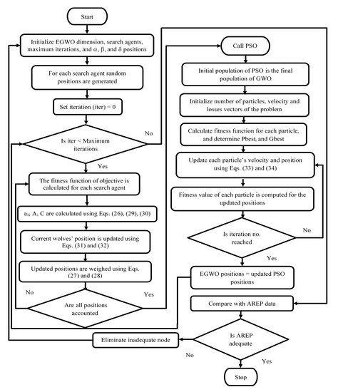
Figure 1.
Flowchart of the AREP-EGWO-PSO method.
As bus number 1 is taken as the slack bus, the potential of PV, WT, and GT DG’s are assessed for the remaining buses in the system. The simulation can be terminated when it satisfies the stopping criterion and displays the re-allocated DG units of the distribution network while fulfilling all the constraints. The details of AREP for IEEE 33 and 69 bus systems are shown in Appendix A and Appendix B, respectively.
5. Case Study
The standard IEEE 33- and 69-bus radial distribution networks are considered to study the proposed AREP-based EGWO-PSO algorithm’s effectiveness, as illustrated in Figure 2 [16]. A simulation study was carried out using MATLAB, and MATPOWER was used to carry out the power flow simulations [44].
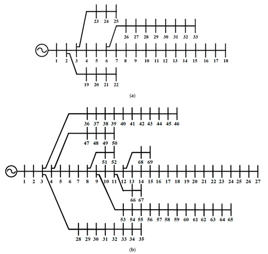
Figure 2.
Topology of (a) 33-bus (b) 69-bus radial distribution network.
To validate the performance of the AREP-EGWO-PSO algorithm, five operational cases are presented for the optimal allocation of DGs. In this study, the EGWO-PSO technique allocates DGs/CBs initially, and the proposed algorithm re-allocates the DG’s based on AREP at various nodes of the distribution system except slack bus. Further, the optimal siting and sizing of CBs obtained by EGWO-PSO are retained for cases 2, 4, and 5.
- Case 1: Optimal allocation of DGs at UPF
- Case 2: Optimal allocation of DGs at UPF with fixed CBs
- Case 3: Optimal allocation of DGs at Lagging/leading power factor (LPF)
- Case 4: Optimal allocation of DGs at LPF with fixed CBs
Three technical objectives (obj1, obj2, obj3) are evaluated for the above cases (1 to 4). The multi-objective function can be constructed using Equation (36):
MOBJ1 = min (obj1, obj2, obj3).
- Case 5: Optimal allocation of multi-DGs with fixed CBs
In this case, three different combinations of eq] (obj1, obj4, and obj5) are taken into account, and their MOBJ can be stated using Equation (37):
MOBJ2 = min (obj1, obj4, obj5).
Different types of DGs have distinct properties of economic and environmental factors. Three DGs of a kind such as PV, WT, and GT are considered, as shown in Table 2. Moreover, substation-generated power cost is assumed as 0.044 $/kWh, and Pi and Ii are deemed to be 30 and 1000 $/kVAR, respectively [29].
Table 2.
Characteristics of DGs.
6. Results and Discussions
To show the effectiveness of the proposed AREP-based algorithm in an optimal allocation of DGs, the IEEE 33-bus and IEEE 69-bus test systems were utilized. Type I and Type III DG units were considered for the analysis. The algorithm was executed with the number of wolves or size of the population, which was 30, and it stopped when the maximum iteration number reached 50. The PSO algorithm considers inertia weight as 1, and social and cognitive component weights are the same, i.e., 2 [45]. Moreover, per unit (p.u.) system was used in all the calculations. The AREP-EGWO-PSO approach and the power-flow solution were executed using the software package MATPOWER 7.0 [44] embedded in MATLAB 2018a software with a configuration of i5 CPU, 1.60 GHz, 8.00 GB RAM, 4-bit operating system. The following sections analyze the results of the various test cases considered.
6.1. IEEE 33-Bus System
The standard IEEE 33-bus distribution network comprises of 33 buses and 32 radial distribution lines. The net complex power loads are 3.72 MW + j 2.3 MVAR [29]. The base values of 100 MVA and 12.66 kV are considered in this study. The voltage level of load buses declines towards the end node. The DGs and CBs are used to enhance the voltage profiles of various buses, thereby reducing the current flows and line losses. Moreover, the uncompensated real power loss for this distribution network is observed as 202.68 kW.
6.1.1. Case 1
Simulation results of the suggested AREP-EGWO-PSO method in comparison with existing optimization techniques are shown in Table 3. It was perceived that the EGWO-PSO algorithm allocates three DGs, initially with sizing 0.754, 1.099, and 1.071 MW at buses 14, 24, and 30, respectively. Since the AREP at bus numbers 14 and 30 are inadequate (Appendix A), the proposed method eliminates these two buses and re-allocates the DGs at new buses 13, 24, and 31 with penetration of 0.823, 1.121, and 0.934 MW, respectively. Under these operating conditions, active power loss becomes 72.53 kW, and minimum voltage occurs at node 30, though with an improved value of 0.970 p.u. The VDI is reduced from its original value to 0.0140 p.u. and VSI is improved from the base value to 0.8871 p.u.
Table 3.
Case 1 of 33-bus system with DGs operating at UPF.
6.1.2. Case 2
Table 4 demonstrates the output result of the EGWO-PSO technique that installs the DGs at buses 14, 24, and 30 and CBs at buses 11, 23, and 29, respectively. The proposed algorithm reserves the allocation of CBs and checks the AREP only for DG buses. On account of deficient AREP at nodes 14 and 30, these nodes are eliminated, and the proposed algorithm re-allocates the DGs at new nodes, namely 13, 24, and 31, with capacities of 0.811, 1.098, and 0.921 MW, respectively. When compared with other algorithms, power loss reduction of 16.001 kW is accomplished by the proposed algorithm. The bus voltage is minimum at bus 22 with 0.994 p.u. Additionally, VDI decreases from its base value to 0.0004 p.u. VSI is further improved to 0.9767 p.u.
Table 4.
Case 2 of 33-bus system with DGs operating at UPF and CBs.
6.1.3. Case 3
In the cases mentioned above, the DGs are disallowed to feed reactive power in the distribution system. Table 5 presents summary of the proposed method simulation results, accompanied by the existing approaches in the literature. From the AREP availability, it is found that there are inadequate capacities at nodes 13 and 30 allotted by the EGWO-PSO method. Then, the proposed technique eradicated these nodes and re-locates the DGs at buses 14, 24, and 31. The total DG size is reduced to 2.820 MW, but active power losses are increased to 15.50 kW. Further, VDI diminishes from 0.1171 p.u. to 0.0009 p.u. and VSI augments from 0.6968 p.u. to 0.9626 p.u. The minimum voltage of 0.991 p.u. is held at the same bus.
Table 5.
Case 3 of 33-bus network with DGs operating at LPF.
6.1.4. Case 4
Similar to case 2, the proposed AREP-EGWO-PSO algorithm retains the optimal allocation of CBs and examines the AREP for DG buses only. Since AREP at nodes 13 and 30 are insufficient, the proposed algorithm eliminates these nodes and re-allocates the DGs at nodes 14, 24, and 32 with penetration of 0.782, 1.109, and 0.909 MW, respectively. The multi-objectives (MOBJ1) are compared with other existing methods, as presented in Table 6. The real power losses increased from 14.99 kW to 16.35 kW, and were obtained through the EGWO-PSO method. The bus voltage is minimum at bus 8 with 0.994 p.u. Furthermore, VDI decreased to 0.0004 p.u. and VSI increased to 0.9762 p.u from their actual values.
Table 6.
Case 4 of 33-bus network with DGs operating at LPF and CB.
6.1.5. Case 5
Table 7 furnishes the multi-objective technical, economic, and environmental benefits (MOBJ2) of DGs allocations in a 33-bus network with pre-allocated CBs. It indicates that the proposed technique eliminates inadequate AREP nodes 13 and 27 and re-allocates the DGs at new nodes 18, 24, 28, and 30. The sizing of renewable DGs is PV at nodes 28 and 30 with 0.7231 MW and 0.59387 MW, respectively, WT at node 24 with 1.0642 MW, and GT at node 18 with 0.50067 MW. As the total sizing of DGs is increased to 2.8863 MW, the power losses, cost of power generated, and total emission all are escalated from the values obtained by the EGWO-PSO algorithm.
Table 7.
Case 5 of 33-bus system with multi-objective placement and sizing.
6.2. IEEE 69-Bus System
This standard distribution network comprises 69 buses with 68 distribution lines with net complex power loads (3.802 MW + j 2.694 MVAR) [29]. The base values of 10 MVA and 12.7 kV are considered. Among 69 buses, the buses 4, 8, 9, 11, and 12 have two branches, and bus 3 has three branches, whereas the remaining buses contain only a single branch associated with their subsequent bus. The uncompensated active power loss for this radial distribution network is observed as 225 kW.
6.2.1. Case 1
The simulation results of the proposed AREP-EGWO-PSO technique for three DGs operating at UPF are shown in Table 8 compared to existing methods. The EGWO-PSO method installs three DGs at buses 11, 18, and 61. Since the AREP is inadequate at nodes 11 and 61, the proposed algorithm removes it and re-allocates three DGs at new buses 18, 60, and 65, with penetration of 0.528, 1.361, and 0.454 MW, respectively. The active power loss is increased to 76.50 kW compared to the EGWO-PSO method. The minimum voltage is observed at node 61, about 0.978 p.u. The VDI decreased from its actual value to 0.0063 p.u. and VSI is augmented to 0.9164 p.u from its base value.
Table 8.
Case 1 of 69-bus system with DGs operating at UPF.
6.2.2. Case 2
In this case, three DGs at UPF are installed at buses 11, 17, and 61, and three CBs at buses 61, 64, and 69 (Table 9). The proposed technique maintains the CBs allocation and compares the AREP for DG buses only. Owing to the lack of AREP at nodes 11 and 61, these nodes are eliminated, and DGs are reinstalled at new nodes, 17, 60, and 65, with a sizing of 0.521, 1.295, and 0.449 MW, respectively, by the proposed algorithm. It is observed that there is an increase in a power loss of 14.12 kW when compared with EGWO-PSO; nevertheless, it is less compared to WCA. The value of VDI is further minimized to 0.0003 p.u. with an augmented VSI scale to 0.9794 p.u.
Table 9.
Case 2 of 69-bus system with DGs operating at UPF and CBs.
6.2.3. Case 3
Table 10 shows the results of the allocation of DGs operating at LPF. Primarily, the EGWO-PSO technique sites the buses at 11, 18, and 61, however buses 11 and 61 are eliminated by the proposed AREP-EGWO-PSO method because of inadequate AREP at these buses. Further, the algorithm re-allocates the DGs at buses 18, 60, and 65 with sizing of 0.516, 1.312, and 0.455 MW, respectively. The suggested method offered a real power loss of 13.98 kW, higher than that of the EGWO-PSO method. The minimum voltage is maintained, similar to case 2. The value of VDI is reduced to 0.0005 p.u. and VSI is increased to 0.9778 p.u. from their actual values.
Table 10.
Case 3 of 33-bus system with DGs operating at LPF.
6.2.4. Case 4
In this case, the optimal allocation of type III DGs with CBs offered better results than in Table 11. The proposed technique reserves the CBs’ allocation and considers the AREP for DG buses only. The buses 11 and 61 are eliminated and new locations are identified as 20, 60, and 65, with DG sizing of 0.492, 1.304, and 0.444 MW, respectively, by the proposed method. The re-allocation of DGs increased the active power losses from 7.21 kW to 13.64 kW. The VDI is further decreased to 0.0002 p.u with an increased VSI value of about 0.9794 p.u. from their actual values.
Table 11.
Case 4 of 69-bus system with DGs operating at LPF and CB.
6.2.5. Case 5
The multi-objective technical, economic, and environmental benefits (MOBJ2) of the allocation of multiple DGs with CBs are shown in Table 12. The proposed method eliminates the insufficient AREP DG buses 11 and 63 and re-locates the DGs at 23, 60, 61, and 64 with total penetration of 2.212 MW. Notably, the active power losses, production costs, and pollutant emissions are lower than WCA but are higher than EGWO-PSO algorithms due to the re-allocation.
Table 12.
Case 5 of 69-bus system with multi-objective placement and sizing.
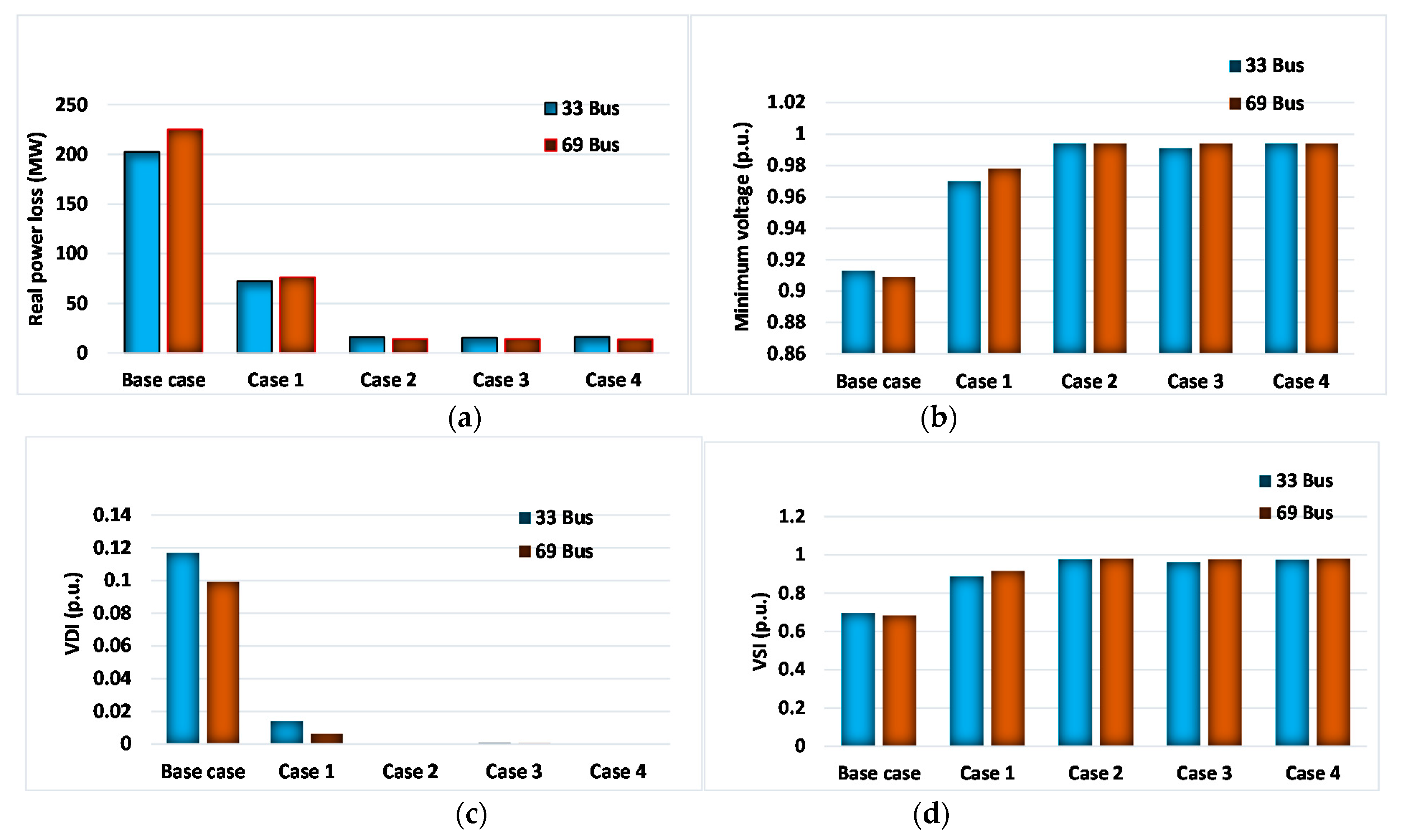
6.3. Comparative Analysis
A comparative study of active power loss, minimum bus voltage magnitude, VDI, and VSI for cases 1 to 4 of IEEE standard 33 and 69 radial distribution systems are shown in Figure 3. The simulation results indicate that the DGs operating at LPF with CBs (Case 4) minimizes the real power losses and voltage deviation and maximizes VSI compared with other cases. The minimum bus voltage level is improved in all the cases after the optimal re-allocation of DGs with/without CBs.

Figure 3.
Comparative study: (a) real power loss; (b) minimum voltage; (c) VDI; (d) VSI.
Further analysis is carried out for best case from four cases, i.e., case 4 (optimal allocation of DGs at LPF with fixed CBs). The voltage profiles before and after re-allocation of DGs are shown in Figure 4 for 33 and 69-bus RDSs. It is noticed that the voltage level is maintained at almost the same level for before and after re-allocation.
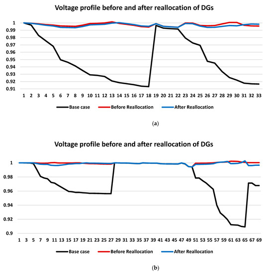
Figure 4.
Voltage profile before and after re-allocation of DGs: (a) 33-bus; (b) 69-bus.
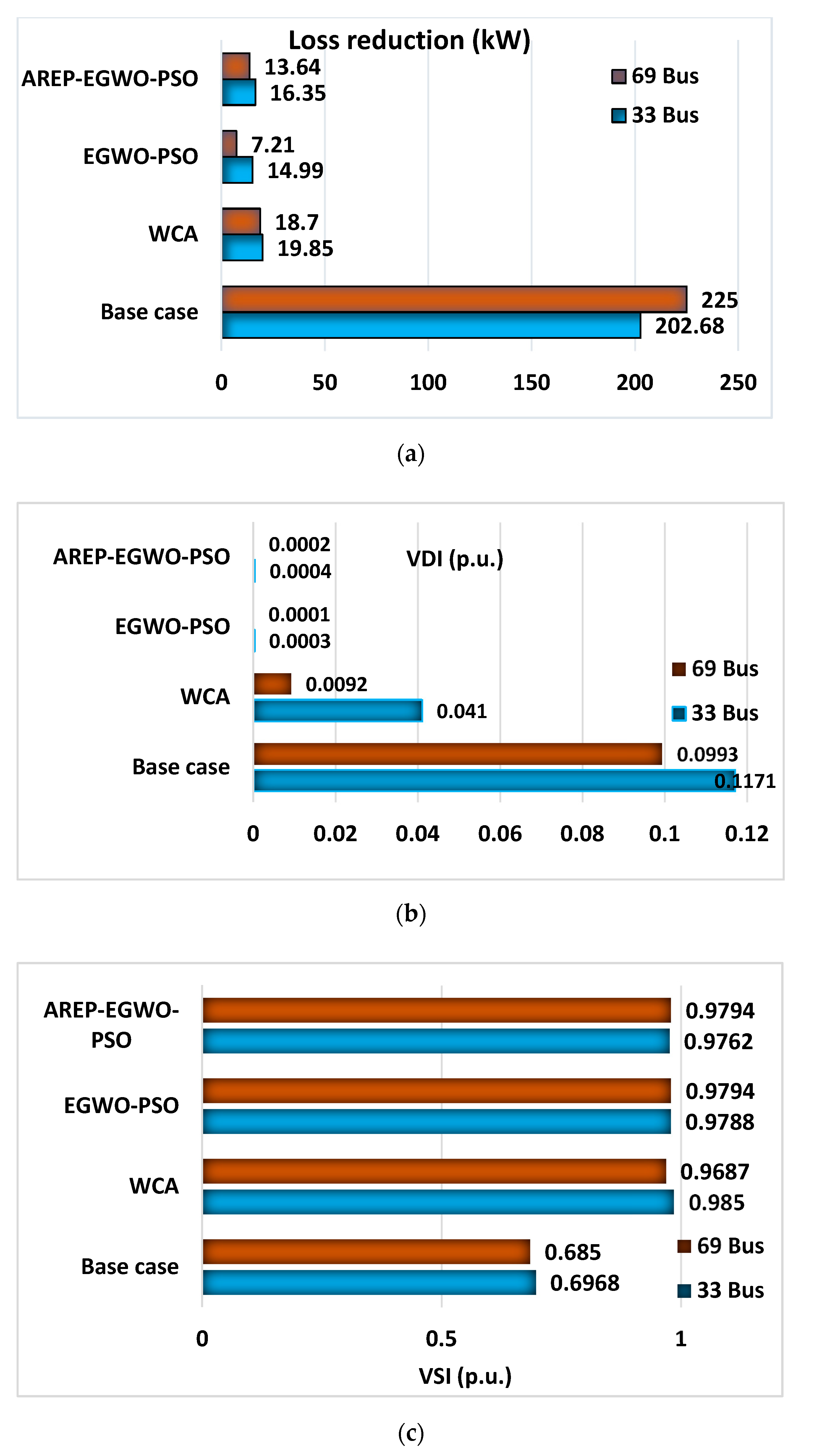
The technical objectives, i.e., real power losses, VDI minimization, and VSI maximization, are shown in Figure 5 for the best case.

Figure 5.
Technical objectives for case 4: (a) loss reduction; (b) VDI minimization; (c) VSI maximization.
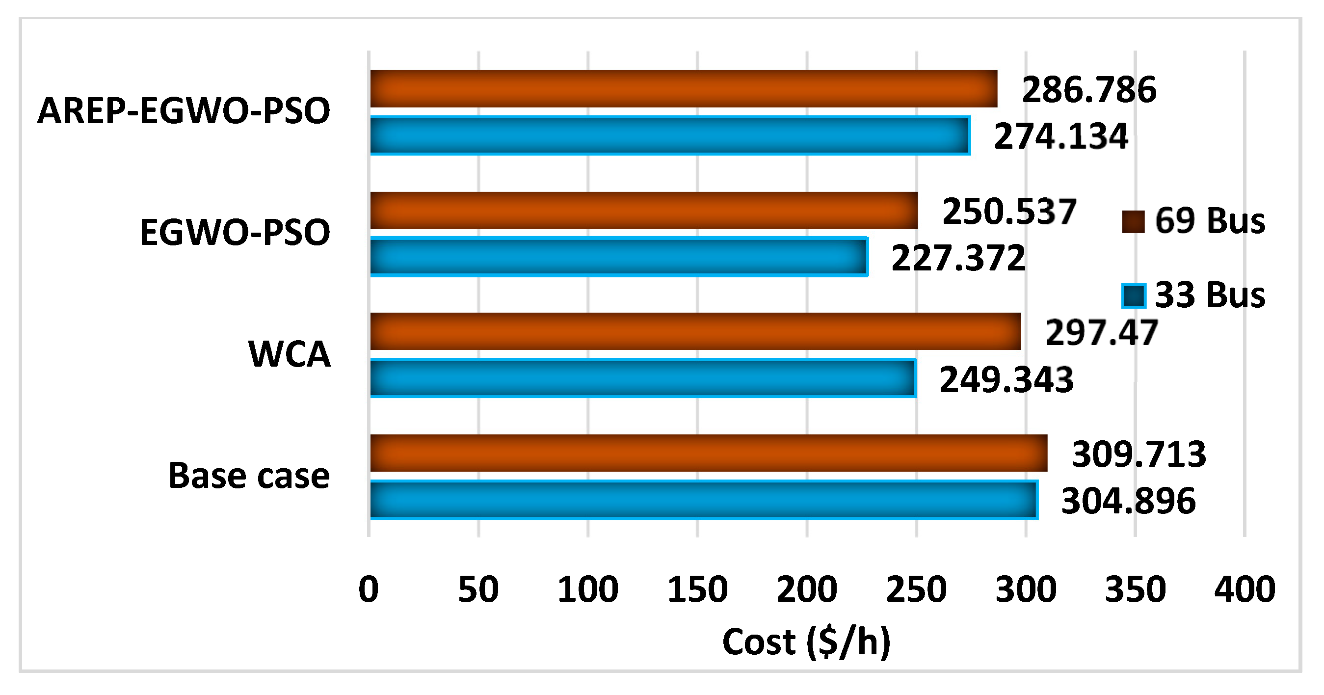
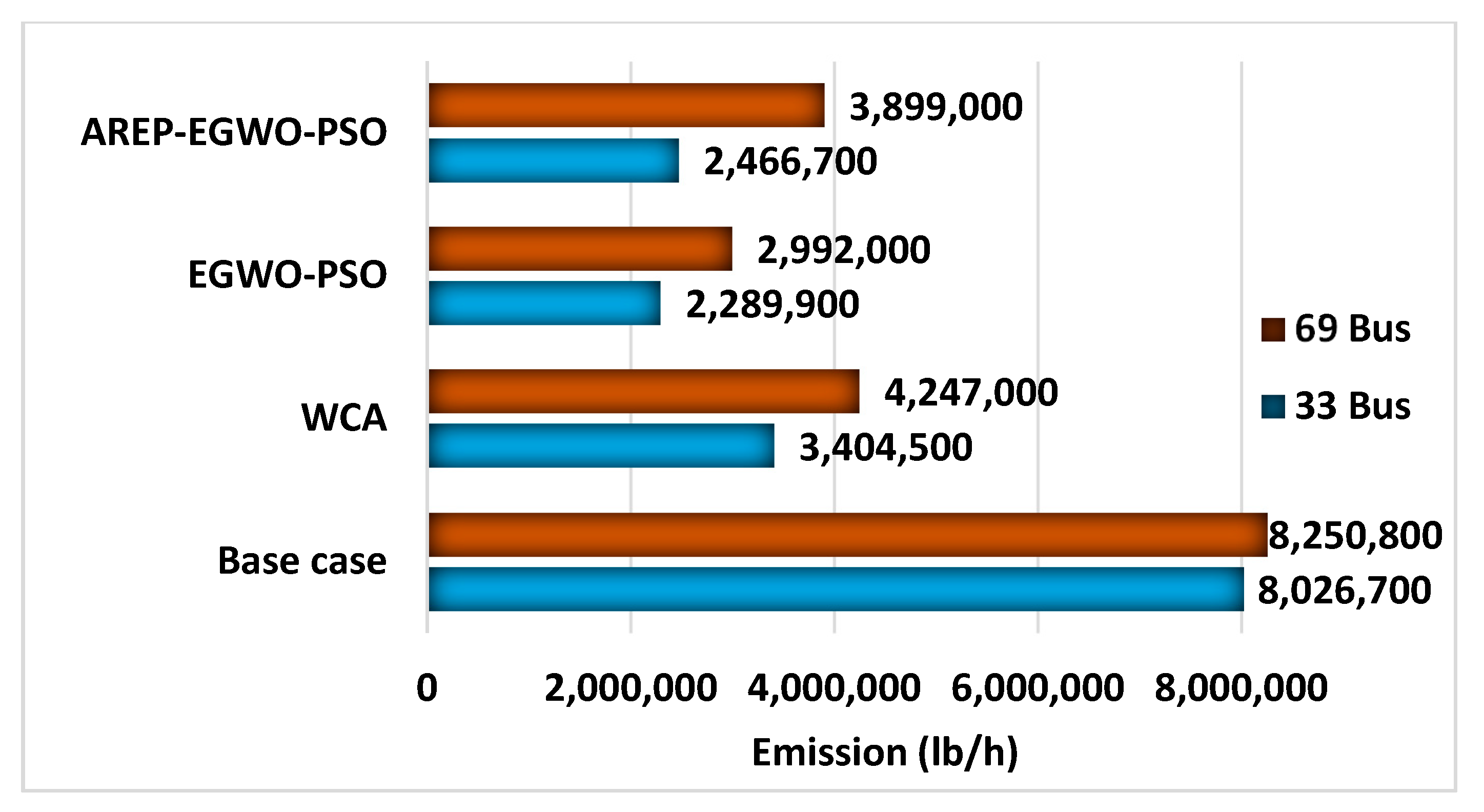
Further, the economic and environmental objectives for case 4 are shown in Figure 6 and Figure 7, respectively. It is observed that the proposed re-allocation procedure shows superior performance compared with other existing methodologies and exhibits almost similar concert with the EGWO-PSO after re-allocation.

Figure 6.
Economic objective for case 4.

Figure 7.
Environmental objective for case 4.
The proposed AREP-EGWO-PSO technique delivers a better solution to the different technical objectives, i.e., real power losses, VDI minimization, and VSI maximization, economic and environmental objectives in the various cases considered. It maintains the same consistency as that of the EGWO-PSO method in achieving all these objectives. The proposed method can be implemented to allocate the DGs in any practical system with the most optimal solutions using available renewable resources.
7. Conclusions
An AREP-based hybrid EGWO-PSO technique was proposed as a multi-criterion-multi-objective framework for the optimal re-allocation and re-sizing of DGs in distribution systems. It was observed that the AREP-EGWO-PSO technique could effectively re-allocate the DGs and re-size the capacity optimally. Notably, real power loss of the system was condensed significantly by up to 92.35% and 93.94% for 33 and 69 test systems, respectively, using AREP constraints. Further, the VSI of the system was greatly enhanced from its base value. Moreover, an excellent emission reduction had taken place by up to 69%, with a significant cost reduction of up to 10%. All these observed outcomes show superior performance compared with other existing optimization techniques. Notably, the AREP-based re-allocation and re-sizing of DGs offer closer performance with EGWO-PSO in all criteria (technical, economic, and environmental). Therefore, the AREP-based re-allocation and re-sizing of DGs using the EGWO-PSO algorithm can be employed to solve complex multi-objective problems for real-time systems.
The future developments accredited to dynamic load variations can be analyzed from the perspective of optimal power system operation. This research work can be extended to include reliability metrices with a reconfiguration of the distribution system. Moreover, a real-time potential assessment of an existing power system can be performed along with the reallocation of DGs based on AREP to validate the effectiveness of the proposed EGWO-PSO algorithm.
Author Contributions
Conceptualization, C.V. and R.K.; methodology, C.V. and R.K.; software, C.V. and R.K.; validation, C.V. and R.K.; formal analysis, D.R.; investigation, V.L.; Supervision, M.H.A., Z.W.G. and J.H.; Writing—original draft, C.V., R.K. and V.L.; Writing—review and editing, M.H.A., Z.W.G., J.H. and D.C.; Funding, Z.W.G. and J.H. All authors have read and agreed to the published version of the manuscript.
Funding
This research was supported by the Energy Cloud R&D Program through the National Research Foundation of Korea (NRF) funded by the Ministry of Science, ICT (2019M3F2A1073164).
Institutional Review Board Statement
Not applicable.
Informed Consent Statement
Not applicable.
Data Availability Statement
Not applicable.
Conflicts of Interest
The authors declare no conflict of interest.
Appendix A
Table A1.
AREP Data for IEEE 33-Bus System.
Table A1.
AREP Data for IEEE 33-Bus System.
| ‘Bus No’ | ‘PV’ | ‘WT’ | ‘GT’ |
|---|---|---|---|
| 2 | 1.416811 | 0.14859 | 0.725957 |
| 3 | 1.618209 | 1.831352 | 1.649998 |
| 4 | 0.968719 | 1.950474 | 1.617671 |
| 5 | 0.778194 | 1.353325 | 0.112631 |
| 5 | 0.928099 | 1.358976 | 0.094402 |
| 7 | 1.385327 | 1.779761 | 1.034487 |
| 8 | 0.461034 | 0.818609 | 0.223704 |
| 9 | 0.34476 | 1.779539 | 1.088131 |
| 10 | 1.523637 | 1.368845 | 1.283628 |
| 11 | 0.911622 | 1.140432 | 0.23583 |
| 12 | 1.150228 | 0.460206 | 0.498481 |
| 13 | 0.1256 | 0.1514 | 0.2128 |
| 14 | 0.1147 | 0.2136 | 0.3249 |
| 15 | 1.114726 | 0.125897 | 1.83734 |
| 16 | 1.368482 | 1.946823 | 0.161324 |
| 17 | 0.214187 | 1.024223 | 1.804306 |
| 18 | 0.774483 | 1.159366 | 1.385843 |
| 19 | 0.631677 | 0.332454 | 0.447655 |
| 20 | 0.358377 | 1.828926 | 1.542147 |
| 21 | 0.090268 | 0.633536 | 1.580214 |
| 22 | 1.724825 | 0.607015 | 1.556447 |
| 23 | 1.958863 | 0.057297 | 1.668655 |
| 24 | 1.464163 | 1.552195 | 1.160197 |
| 25 | 0.1626 | 1.2106 | 0.8399 |
| 26 | 0.571004 | 1.286817 | 1.964925 |
| 27 | 0.404072 | 0.284293 | 0.304324 |
| 28 | 1.118003 | 1.741504 | 0.114022 |
| 29 | 0.8989 | 1.5806 | 1.4299 |
| 30 | 0.1432 | 0.2658 | 0.3146 |
| 31 | 0.74843 | 0.397773 | 0.080544 |
| 32 | 1.154837 | 1.006679 | 0.660426 |
| 33 | 1.244935 | 0.933108 | 1.390878 |
Appendix B
Table A2.
AREP Data for IEEE 69-Bus System.
Table A2.
AREP Data for IEEE 69-Bus System.
| ‘Bus No’ | ‘PV’ | ‘WT’ | ‘GT’ |
|---|---|---|---|
| 2 | 0.2986 | 1.7386 | 0.7015 |
| 3 | 0.515 | 1.1594 | 1.878 |
| 4 | 1.6814 | 1.0997 | 1.7519 |
| 5 | 0.5086 | 0.2899 | 1.1003 |
| 5 | 1.6286 | 1.7061 | 1.245 |
| 7 | 0.487 | 1.2441 | 1.1741 |
| 8 | 1.8585 | 0.7019 | 0.4155 |
| 9 | 0.723 | 1.0265 | 0.6025 |
| 10 | 0.3932 | 0.8036 | 0.9418 |
| 11 | 0.1215 | 0.1532 | 0.2146 |
| 12 | 1.2321 | 0.4798 | 1.6886 |
| 13 | 0.9466 | 0.2466 | 0.3895 |
| 14 | 0.7033 | 0.3678 | 0.4518 |
| 15 | 1.6617 | 0.4799 | 0.3414 |
| 16 | 1.1705 | 0.8345 | 0.4553 |
| 17 | 1.0994 | 0.0993 | 0.8714 |
| 18 | 1.8344 | 1.8054 | 0.6222 |
| 19 | 0.5717 | 1.8896 | 1.8468 |
| 20 | 1.5144 | 0.9817 | 0.8604 |
| 21 | 1.5075 | 0.9785 | 0.3696 |
| 22 | 0.7609 | 0.6754 | 1.8098 |
| 23 | 1.1356 | 1.8001 | 1.9595 |
| 24 | 0.1517 | 0.7385 | 0.8777 |
| 25 | 0.1079 | 0.2224 | 0.2222 |
| 26 | 1.0616 | 1.5605 | 0.5161 |
| 27 | 1.5583 | 0.7795 | 0.8174 |
| 28 | 1.868 | 0.4834 | 1.1898 |
| 29 | 0.2598 | 0.8078 | 0.5244 |
| 30 | 1.1376 | 0.1929 | 1.2057 |
| 31 | 0.9388 | 0.2639 | 1.4224 |
| 32 | 0.0238 | 1.8841 | 0.4435 |
| 33 | 0.6742 | 1.9123 | 0.2348 |
| 34 | 0.3244 | 1.1504 | 0.5934 |
| 35 | 1.5886 | 0.1196 | 0.6376 |
| 36 | 0.6224 | 0.4696 | 0.8483 |
| 37 | 1.0571 | 0.7063 | 1.0157 |
| 38 | 0.3313 | 1.6424 | 0.171 |
| 39 | 1.204 | 0.0308 | 0.525 |
| 40 | 0.5259 | 0.086 | 1.602 |
| 41 | 1.3082 | 0.338 | 0.0584 |
| 42 | 1.3784 | 1.2982 | 1.8577 |
| 43 | 1.4963 | 1.4634 | 1.4607 |
| 44 | 0.9011 | 1.2955 | 0.9772 |
| 45 | 0.1676 | 0.9018 | 1.1571 |
| 46 | 0.458 | 1.094 | 0.4746 |
| 47 | 1.8267 | 0.5926 | 0.9177 |
| 48 | 0.3048 | 1.4894 | 1.9262 |
| 49 | 1.6516 | 0.3779 | 1.0936 |
| 50 | 1.0767 | 1.3736 | 1.0423 |
| 51 | 1.9923 | 0.367 | 0.4632 |
| 52 | 0.1564 | 0.737 | 0.9778 |
| 53 | 0.8854 | 1.2512 | 1.2481 |
| 54 | 0.2133 | 1.5605 | 1.3583 |
| 55 | 1.9238 | 0.1623 | 0.791 |
| 56 | 0.0093 | 1.8588 | 0.7349 |
| 57 | 1.5498 | 1.5514 | 1.976 |
| 58 | 1.6346 | 0.9736 | 0.0755 |
| 59 | 1.7374 | 0.8717 | 1.7703 |
| 60 | 0.922 | 0.6564 | 0.7402 |
| 61 | 0.1321 | 0.2021 | 0.3211 |
| 62 | 0.5197 | 1.017 | 0.1974 |
| 63 | 0.1232 | 0.2123 | 0.3135 |
| 64 | 0.8628 | 1.6353 | 0.6707 |
| 65 | 1.8213 | 1.5897 | 1.3595 |
| 66 | 0.3637 | 1.2886 | 0.2731 |
| 67 | 0.5276 | 0.7572 | 1.4425 |
| 68 | 0.2911 | 1.6232 | 0.2135 |
| 69 | 0.2721 | 1.0657 | 1.3075 |
References
- HA, M.P.; Nazari-Heris, M.; Mohammadi-Ivatloo, B.; Seyedi, H. A hybrid genetic particle swarm optimization for distributed generation allocation in power distribution networks. Energy 2020, 209, 118218. [Google Scholar] [CrossRef]
- Rao, R.S.; Ravindra, K.; Satish, K.; Narasimham, S.V.L. Power Loss Minimization in Distribution System Using Network Reconfiguration in the Presence of Distributed Generation. IEEE Trans. Power Syst. 2013, 28, 317–325. [Google Scholar] [CrossRef]
- Pereira, B.R.; Da Costa, G.R.M.M.; Contreras, J.; Mantovani, J.R.S. Optimal Distributed Generation and Reactive Power Allocation in Electrical Distribution Systems. IEEE Trans. Sustain. Energy 2016, 7, 975–984. [Google Scholar] [CrossRef] [Green Version]
- Bawazir, R.O.; Cetin, N.S. Comprehensive overview of optimizing PV-DG allocation in power system and solar energy resource potential assessments. Energy Rep. 2020, 6, 173–208. [Google Scholar] [CrossRef]
- Morsali, R.; Ghadimi, N.; Karimi, M.; Mohajeryami, S. Solving a novel multiobjective placement problem of recloser and distributed generation sources in simultaneous mode by improved harmony search algorithm. Complexity 2015, 21, 328–339. [Google Scholar] [CrossRef]
- Sheng, W.; Liu, K.; Liu, Y.; Ye, X.; He, K. Reactive power coordinated optimisation method with renewable distributed generation based on improved harmony search. IET Gener. Transm. Distrib. 2016, 10, 3152–3162. [Google Scholar] [CrossRef]
- Shaheen, A.M.; El-Sehiemy, R.A. Optimal Coordinated Allocation of Distributed Generation Units/Capacitor Banks/Voltage Regulators by EGWA. IEEE Syst. J. 2021, 15, 257–264. [Google Scholar] [CrossRef]
- Diab, A.A.Z.; Rezk, H. Optimal Sizing and Placement of Capacitors in Radial Distribution Systems Based on Grey Wolf, Dragonfly and Moth–Flame Optimization Algorithms. Iran J. Sci. Technol. Trans. Electr. Eng. 2019, 43, 77–96. [Google Scholar] [CrossRef]
- Rajendran, A.; Narayanan, K. Multi-Objective Hybrid WIPSO–GSA Algorithm-Based DG and Capacitor Planning for Reduction of Power Loss and Voltage Deviation in Distribution System. Smart Sci. 2018, 6, 295–307. [Google Scholar] [CrossRef]
- Montazeri, M.; Askarzadeh, A. Capacitor placement in radial distribution networks based on identification of high potential busses. Int. Trans. Electr. Energy Syst. 2019, 29, e2754. [Google Scholar] [CrossRef]
- Sanjay, R.; Jayabarathi, T.; Raghunathan, T.; Ramesh, V.; Mithulananthan, N. Optimal Allocation of Distributed Generation Using Hybrid Grey Wolf Optimizer. IEEE Access 2017, 5, 14807–14818. [Google Scholar] [CrossRef]
- Quadri, I.A.; Bhowmick, S.; Joshi, D. A hybrid teaching–learning-based optimization technique for optimal DG sizing and placement in radial distribution systems. Soft Comput. 2019, 23, 9899–9917. [Google Scholar] [CrossRef]
- Bayat, S.A.; Davoudkhani, I.F.; Moghaddam, M.J.H.; Najmi, E.S.; Abdelaziz, A.Y.; Ahmadi, A.; Razavi, S.E.; Gandoman, F.H. Fuzzy multi-objective placement of renewable energy sources in distribution system with objective of loss reduction and reliability improvement using a novel hybrid method. Appl. Soft Comput. 2019, 77, 761–779. [Google Scholar]
- Arif, S.M.; Hussain, A.; Lie, T.T.; Ahsan, S.M.; Khan, H.A. Analytical Hybrid Particle Swarm Optimization Algorithm for Optimal Siting and Sizing of Distributed Generation in Smart Grid. J. Mod. Power Syst. Clean Energy 2020, 8, 1221–1230. [Google Scholar] [CrossRef]
- Yang, B.; Yu, L.; Chen, Y.; Ye, H.; Shao, R.; Shu, H.; Yu, T.; Zhang, X.; Sun, L. Modelling, applications, and evaluations of optimal sizing and placement of distributed generations: A critical state-of-the-art survey. Int. J. Energy Res. 2020, 45, 3615–3642. [Google Scholar] [CrossRef]
- Venkatesan, C.; Kannadasan, R.; Alsharif, M.; Kim, M.-K.; Nebhen, J. A Novel Multiobjective Hybrid Technique for Siting and Sizing of Distributed Generation and Capacitor Banks in Radial Distribution Systems. Sustainability 2021, 13, 3308. [Google Scholar] [CrossRef]
- Taha, I.B.M.; Elattar, E.E. Optimal reactive power resources sizing for power system operations enhancement based on improved grey wolf optimiser. IET Gener. Transm. Distrib. 2018, 12, 3421–3434. [Google Scholar] [CrossRef]
- Das, S.; Das, D.; Patra, A. Operation of distribution network with optimal placement and sizing of dispatchable DGs and shunt capacitors. Renew. Sustain. Energy Rev. 2019, 113, 109219. [Google Scholar] [CrossRef]
- Suresh, M.; Edward, J.B. A hybrid algorithm based optimal placement of DG units for loss reduction in the distribution system. Appl. Soft Comput. 2020, 91, 106191. [Google Scholar] [CrossRef]
- Muthukumar, K.; Jayalalitha, M. Integrated approach of network reconfiguration with distributed generation and shunt capacitors placement for power loss minimization in radial distribution networks. Appl. Soft Comput. 2017, 52, 1262–1284. [Google Scholar] [CrossRef]
- El-Salam, M.F.A.; Beshr, E.; Eteiba, M. A New Hybrid Technique for Minimizing Power Losses in a Distribution System by Optimal Sizing and Siting of Distributed Generators with Network Reconfiguration. Energies 2018, 11, 3351. [Google Scholar] [CrossRef] [Green Version]
- Alzaidi, K.M.S.; Bayat, O.; Uçan, O.N. Multiple DGs for Reducing Total Power Losses in Radial Distribution Systems Using Hybrid WOA-SSA Algorithm. Int. J. Photoenergy 2019, 2019, 2426538. [Google Scholar] [CrossRef]
- Arulraj, R.; Kumarappan, N. Optimal economic-driven planning of multiple DG and capacitor in distribution network considering different compensation coefficients in feeder’s failure rate evaluation. Eng. Sci. Technol. Int. J. 2019, 22, 67–77. [Google Scholar] [CrossRef]
- Angalaeswari, S.; Sanjeevikumar, P.; Jamuna, K.; Leonowicz, Z. Hybrid PIPSO-SQP Algorithm for Real Power Loss Minimization in Radial Distribution Systems with Optimal Placement of Distributed Generation. Sustainability 2020, 12, 5787. [Google Scholar] [CrossRef]
- Milovanović, M.; Tasić, D.; Radosavljević, J.; Perović, B. Optimal Placement and Sizing of Inverter-Based Distributed Generation Units and Shunt Capacitors in Distorted Distribution Systems Using a Hybrid Phasor Particle Swarm Optimization and Gravitational Search Algorithm. Electr. Power Compon. Syst. 2020, 48, 543–557. [Google Scholar] [CrossRef]
- Montoya, O.D.; Gil-González, W.; Orozco-Henao, C. Vortex search and Chu-Beasley genetic algorithms for optimal location and sizing of distributed generators in distribution networks: A novel hybrid approach. Eng. Sci. Technol. Int. J. 2020, 23, 1351–1363. [Google Scholar] [CrossRef]
- Coelho, F.C.R.; Junior, I.C.D.S.; Dias, B.H.; Peres, W.; Ferreira, V.H.; Marcato, A.L.M. Optimal distributed generation allocation in unbalanced radial distribution networks via empirical discrete metaheuristic and steepest descent method. Electr. Eng. 2021, 103, 633–646. [Google Scholar] [CrossRef]
- Venkatesan, C.; Kannadasan, R.; Alsharif, M.; Kim, M.-K.; Nebhen, J. Assessment and Integration of Renewable Energy Resources Installations with Reactive Power Compensator in Indian Utility Power System Network. Electronics 2021, 10, 912. [Google Scholar] [CrossRef]
- El-Ela, A.A.A.; El-Sehiemy, R.A.; Abbas, A.S. Optimal Placement and Sizing of Distributed Generation and Capacitor Banks in Distribution Systems Using Water Cycle Algorithm. IEEE Syst. J. 2018, 12, 3629–3636. [Google Scholar] [CrossRef]
- Ali, A.U.; Keerio, M.U.; Laghari, J.A. Optimal Site and Size of Distributed Generation Allocation in Radial Distribution Network Using Multi-objective Optimization. J. Mod. Power Syst. Clean Energy 2021, 9, 404–415. [Google Scholar] [CrossRef]
- Palanisamy, R.; Muthusamy, S.K. Optimal Siting and Sizing of Multiple Distributed Generation Units in Radial Distribution System Using Ant Lion Optimization Algorithm. J. Electr. Eng. Technol. 2021, 16, 79–89. [Google Scholar] [CrossRef]
- Abdelaziz, A.; Ali, E.; Elazim, S.A. Flower Pollination Algorithm and Loss Sensitivity Factors for optimal sizing and placement of capacitors in radial distribution systems. Int. J. Electr. Power Energy Syst. 2016, 78, 207–214. [Google Scholar] [CrossRef]
- Oliveira, V.Y.M.; Oliveira, R.M.S.; Affonso, C.M. Cuckoo Search approach enhanced with genetic replacement of abandoned nests applied to optimal allocation of distributed generation units. IET Gener. Transm. Distrib. 2018, 12, 3353–3362. [Google Scholar] [CrossRef]
- Quadri, I.A.; Bhowmick, S.; Joshi, D. A comprehensive technique for optimal allocation of distributed energy resources in radial distribution systems. Appl. Energy 2018, 211, 1245–1260. [Google Scholar] [CrossRef]
- Pasha, A.M.; Zeineldin, H.H.; El-Saadany, E.F.; Alkaabi, S.S. Optimal allocation of distributed generation for planning master–slave controlled microgrids. IET Gener. Transm. Distrib. 2019, 13, 3704–3712. [Google Scholar] [CrossRef]
- Muthukumar, K.; Jayalalitha, S. Optimal placement and sizing of distributed generators and shunt capacitors for power loss minimization in radial distribution networks using hybrid heuristic search optimization technique. Int. J. Electr. Power Energy Syst. 2016, 78, 299–319. [Google Scholar] [CrossRef]
- Murthy, V.; Kumar, A. Comparison of optimal DG allocation methods in radial distribution systems based on sensitivity approaches. Int. J. Electr. Power Energy Syst. 2013, 53, 450–467. [Google Scholar] [CrossRef]
- Sadiq, A.; Adamu, S.; Buhari, M. Optimal distributed generation planning in distribution networks: A comparison of transmission network models with FACTS. Eng. Sci. Technol. Int. J. 2019, 22, 33–46. [Google Scholar] [CrossRef]
- Poornazaryan, B.; Karimyan, P.; Gharehpetian, G.; Abedi, M. Optimal allocation and sizing of DG units considering voltage stability, losses and load variations. Int. J. Electr. Power Energy Syst. 2016, 79, 42–52. [Google Scholar] [CrossRef]
- Mirjalili, S.; Mirjalili, S.M.; Lewis, A. Grey wolf optimizer. Adv. Eng. Softw. 2014, 69, 46–61. [Google Scholar] [CrossRef] [Green Version]
- Şenel, F.A.; Gökçe, F.; Yüksel, A.S.; Yiğit, T. A novel hybrid PSO–GWO algorithm for optimization problems. Eng. Comput. 2019, 35, 1359–1373. [Google Scholar] [CrossRef]
- Abdelshafy, A.M.; Hassan, H.; Jurasz, J. Optimal design of a grid-connected desalination plant powered by renewable energy resources using a hybrid PSO–GWO approach. Energy Convers. Manag. 2018, 173, 331–347. [Google Scholar] [CrossRef]
- Ramadan, H.; Bendary, A.; Nagy, S. Particle swarm optimization algorithm for capacitor allocation problem in distribution systems with wind turbine generators. Int. J. Electr. Power Energy Syst. 2017, 84, 143–152. [Google Scholar] [CrossRef]
- Zimmerman, R.D.; Murillo-Sanchez, C.E. Matpower [Software]. Available online: https://matpower.org (accessed on 20 September 2021). [CrossRef]
- Kumar, S.; Mandal, K.; Chakraborty, N. Optimal DG placement by multi-objective opposition based chaotic differential evolution for techno-economic analysis. Appl. Soft Comput. 2019, 78, 70–83. [Google Scholar] [CrossRef]
- Sultana, S.; Roy, P. Multi-objective quasi-oppositional teaching learning based optimization for optimal location of distributed generator in radial distribution systems. Int. J. Electr. Power Energy Syst. 2014, 63, 534–545. [Google Scholar] [CrossRef]
- Moradi, M.H.; Abedini, M. A combination of genetic algorithm and particle swarm optimization for optimal DG location and sizing in distribution systems. Int. J. Electr. Power Energy Syst. 2012, 34, 66–74. [Google Scholar] [CrossRef]
- Mohamed Imran, A.; Kowsalya, M.; Kothari, D.P. A novel integration technique for optimal network reconfiguration and distributed generation placement in power distribution networks. Int. J. Electr. Power Energy Syst. 2014, 63, 461–472. [Google Scholar] [CrossRef]
- Kefayat, M.; Ara, A.L.; Niaki, S.N. A hybrid of ant colony optimization and artificial bee colony algorithm for probabilistic optimal placement and sizing of distributed energy resources. Energy Convers. Manag. 2015, 92, 149–161. [Google Scholar] [CrossRef]
- Injeti, S.K.; Kumar, N.P. A novel approach to identify optimal access point and capacity of multiple DGs in a small, medium and large scale radial distribution systems. Int. J. Electr. Power Energy Syst. 2013, 45, 142–151. [Google Scholar] [CrossRef]


Publisher’s Note: MDPI stays neutral with regard to jurisdictional claims in published maps and institutional affiliations. |
© 2021 by the authors. Licensee MDPI, Basel, Switzerland. This article is an open access article distributed under the terms and conditions of the Creative Commons Attribution (CC BY) license (https://creativecommons.org/licenses/by/4.0/).