Inter- and Intra-Regional Disparities in Russia: Factors of Uneven Economic Growth

Abstract

Despite the growing body of literature on the dependence of economic growth from different factors, the reasons for uneven growth remain unclear. Within the country, regions have different growth rates in their diverse parts. It is unclear why the same factor could influence municipalities differently. To reveal this reason, we used hierarchical linear modeling with spatial dependence, which allows us to decompose variation into regional and municipal scales and take into account spatial autocorrelation. We conducted our research on data for 2239 municipalities within 85 Russian regions in 2019. Our model incorporates 20 factors of economic growth, with 7 at the municipal scale. Cross-interaction estimates established that factors attributed to the regional level determined the relationship between dependent variables (growth rate of production, growth rate of social benefits, and taxable income) at the municipal level and predictors. The influence of initial level, investments in fixed assets, employment on municipal growth varies greatly depending on such regional determinants as economic structure, innovation, human capital, and inequality. This paper adds to the existing literature on uneven economic growth at a smaller scale (municipality) and at the same time helps to rethink inter- and intra-regional disparities.

1. Introduction

Despite numerous insightful studies, issues of uneven development, economic inequality, and their impact on sustainability and growth remain relevant. At present, almost every country faces such challenges. The major problem is that the increase in disparities leads to unbalanced and unsustainable development of an economy. In particular, this problem is common in large countries where regional governance has to consider the diversity of growth factors. In different climatic conditions, resource endowments, and historical contexts of various regions, the government should ensure relatively equal levels of sustainable growth across regions. Thus, academics often compare the northern and southern, western and eastern parts of such countries to find opportunities for the convergence of their development. Breau and Saillant [1] assess income inequality in Canada to reveal pivotal factors that influence spatial disparities. They note that high-income Canadian regions are typically concentrated in the western parts of the country. Chen and Feng [2] suggest that the coastal Chinese provinces have experienced much higher economic growth than the inner provinces because of the economic reforms, which encouraged the coastal provinces’ development. Goodman [3] considers economic growth in the United States to be uneven. His analysis showed that factors important for northeastern and southern cities are at the same time uncorrelated with growth in the Midwest and the west.

Russia is the biggest country, featuring differences in eastern, western, northern, and southern territories’ development [4]. We could distinguish between significant differences in climatic conditions (harsh north and warm south), natural resource endowment (mineral-rich northeastern regions of the country and agriculturally favorable black soil in the southwest), production patterns (Urals, West Siberia), and settlement schemes (higher population density in the west, very low in the north). However, as in other foreign countries, differences manifest not only in geographic location. Many factors cause them; thus, it is impossible to follow the “same size fits all approach”. Academics note that tools which work in leading advanced countries may not be efficient in the lagging ones [5]. Therefore, regional policy increasingly provides for variability across regions according to the type of their development. Cutrini [6] identifies five economic clubs in Europe which have various ways of recovering and structural changes. Quatraro [7] suggests that late-industrialized and early-industrialized regions go through various processes of economic growth. To form management decisions, regional planners in Russia distinguish between the following groups: region leaders and outsiders; agrarian regions and industrial ones [8].

In addition to inter-regional differences, there are intra-regional differences. To reveal them, we should conduct our analysis on a smaller scale [5] on which uneven growth of urban/rural areas, centers, and peripheries in the region manifest themselves. In this case, the emphasis shifts from inter- to intra-regional disparities which become more distinct. For example, the EU has successfully alleviated disparities between member states in average income, but many academics have found that regional inequalities within countries have grown. Kilroy and Ganau [5] established that regional inequalities in the EU have been increasing since the beginning of 2000 at all levels while positive convergence existed across countries. Butkus et al. [9] revealed that variation in GDP per capita within countries mainly remained constant or even grew, but between countries, it decreased. They found that urban and capital regions were growing faster while coastal rural ones were lagging [9]. Uneven economic development in China is also associated with differences between centers and periphery [10], and it has an urban/rural gap [11]. The US also has a distinct urban/rural division [12]. Russia, like other countries, has intra-regional issues related to the differences in the center and periphery, accompanied by migration of population to cities. Thus, to understand the reasons for uneven economic growth, we should conduct our analysis on a smaller scale, as according to Butkus et al. it is less spatially sustainable [9]. The complexity of economic systems is that spatial autocorrelation exists together with differences in their development. Academics identify spatial effects in regional economic growth and suggest that spatial scales of regional data could influence the performance and interpretation of empirical growth models [13]. Moreover, the study of Panzera and Postiglione showed that intra-regional inequalities of surrounding areas could influence the growth of the examined region [14]. The main reason is that the regions are not closed systems, but there are flows of goods, technologies, information, and migration between them. In turn, the spatial relationship can be both positive and negative, indicating the nature of the territories’ connectivity. Thus, given these features, various trajectories of territorial economic growth exist. As many studies are aimed at growth models comparison across different groups of countries and regions, the determinants of economic growth could not be the same for every territorial unit [15].

The significance of economic growth factors depends on the regional environment and spatial context. Our paper adds to the recent fast-growing body of literature on uneven economic growth at a smaller scale using data for 2239 municipalities within 85 Russian regions in 2019. We conducted a deep analysis of the economic growth unevenness, focusing on spatial effects, intergroup and intragroup differences, and their relationship within the framework of multilevel models.

Our analysis is descriptive but contributes to the understanding of the economic growth determinants in regions of various levels and economic structures. It could be used as an initial background to investigate the causal relationships between regional policy, investments, and growth. The paper addressed the following questions: What factors matter in one group of regions but do not matter in the others? How do regional and municipal contexts simultaneously influence municipal growth rates? The listed reasons determine the relevance of this research area, and our aim here is threefold:

(1)

Determine how a region and municipality contribute to the variation of economic growth;

(2)

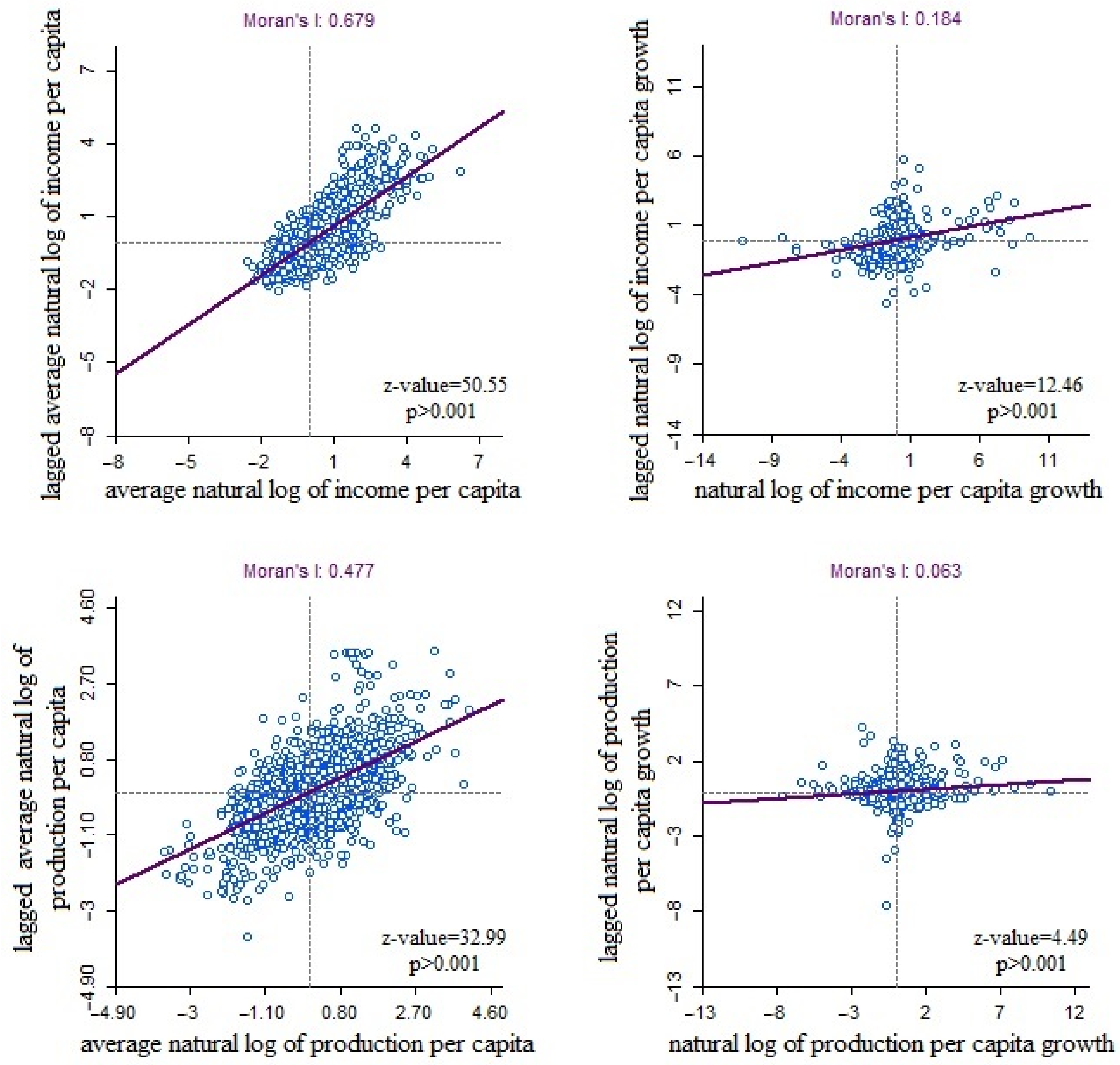
Assess spatial autocorrelation of economic growth;

(3)

Examine how the relationship between economic growth and municipal factors changes depending on included regional features.

The remainder of the paper is organized as follows. Section 2 provides a theoretical framework to investigate uneven economic growth at a small scale and justifies enrolling spatial estimates. Section 3 includes model specifications and data. Section 4 introduces a brief description of the Russian economy and its spatial context. Section 5 provides the main empirical findings, focusing on intra-regional and inter-regional variation. Section 6 presents the discussion. Section 7 concludes the paper.

2. Literature Review

2.1. Uneven Growth at the Small Scale

Uneven growth is an essential feature of many countries [1,3,6,10]. Recent studies address issues of disparities at different administrative scales: national (country), regional (states in USA, Brazil and Australia, provinces in Canada and China, constituent entities in the Russian Federation, NUTS 2 in EU), municipal (counties in USA and China, municipalities in the Russian Federation and Brazil, local government areas in Australia, NUTS3 in EU) and local (cities and villages). The unevenness at the lower level of aggregation is higher in the majority of all cases [9,11,16,17]. The rationale behind this is differences between countries are strengthening with imbalances of development between regions and municipalities. Moreover, some studies show that variation between countries is reducing while inequalities between regions are mostly stagnating or even growing [9].

For instance, Butkus et al. distinguish between disparities of 28 EU countries, within-country disparities at the NUTS 2 level, within-NUTS 2 disparities at the NUTS 3 level, and show that disparities between countries are reducing, but the part of EU disparities that can be attributed to within-country disparities is increasing [9]. Kilroy and Ganau [5] underline the importance of analyzing at the lower level of aggregation, pointing out that disparities are growing at the NUTS-3 level. Regional inequalities at different scales are the focus of Chinese academics. Liao and Wei show that the regional disparities are inconsistent with the geographical scales: inter-county inequalities are higher than inter-municipal and inter-regional ones [11]. These estimates differ for north, west, east, and central regions [18]. He et al. reveal that inequalities between prefectures are higher than within prefectures, within provinces than between provinces, and between regions than within regions in China [16]. Doran and Jordan find that the key trigger of persistent and increasing income inequalities in the US are imbalances in income between counties within states [12]. They associate income inequalities with a strong urban/peripheral division, where more urbanized counties (regardless of the State they are in) gain higher rates of income growth, while counties that are more peripheral lag behind [12]. The above-mentioned reasons raise the importance of analysis at the lower level of data aggregation. However, there is a problem related to the absence of statistics at the sub-regional level. As a result, there are few studies aimed at the analysis of uneven economic growth at a smaller scale (

Table 1. Related studies on economic growth at the small scale.

Research	Research Sample; Analysis Period	Model	Dependent Variable	Independent Variables
Pede [13]	3074 counties in the 48 states of the US; 1990 and 2007	SARAR	per capita income growth	employment diversity, Gini coefficient, amenities, race Black/Hispanic/other, high school grad, some college, associate’s degree, bachelor’s degree, graduate degree, age 5 to 14, age 15 to 17, age 18 to 64, age 65 or over, metropolitan
Higgins et al. [19]	3058 counties of the US; 1970, 1980 and 1990	OLS, CROLS, 3SLS	real per capita income growth	land area per capita, water area per capita, the proportion of the population by age group, percentage of Blacks, Hispanics, education, median house value, poverty, percentage of population employed in the various industries, college town
Fallah & Partridge [20]	3028 counties of the US; 1990 and 2000	GLS	per capita income growth	Gini coefficient, welfare expenditures, initial per capita income, spatial lag per capita income, ethnic diversification, education, natural amenity scale, total poverty rate, the population size, the racial/ethnic composition variables, recent immigrants, age composition shares, and industry composition employment shares
Roth [21]	3117 counties of the US; 1977 and 2000	OLS	per-capita income growth rate	the percent of residents holding a college degree, per-capita housing units constructed, local government spending on public welfare, highways, health, and education, the unemployment rate, voter turnout, percentage of a county’s households that earned less than USD 10,000 and above USD 30,000
Kilroy & Ganau [5]	1348 NUTS-3 regions in the EU; 2003 to 2017	PARDL	GDP per capita growth	industrial structure, innovation, inward FDI, population dynamics and agglomeration forces
Díaz-Dapena et al. [22]	1276 NUTS-3 regions in the EU; 2000 to 2014	OLS, MLM, MLM with spatial dependence	GDP per capita growth	percentage of population with different levels of education, gross capital formation as a percentage of GDP, mean growth of the working population, R&D expenditures as a percentage of GDP
Li & Fang [23]	2286 cities and counties of China; 1992, 2000 and 2010	OLS, SAR, SEM (panel data)	GDP per capita growth	investment return rate, human capital, savings rate, population growth, technology advancement, capital depreciation rate, initial technology level
He et al. [24]	2076 cities and counties of China; from 2000 to 2015	OLS, SLM, SAR, SEM (panel data)	GDP per capita	labor employment, urbanization, urban–rural inequality, fixed investment, industrialization, availability of bank loans, fiscal expenditure decentralization, fiscal autonomy, implementation of “province administering counties” strategy, topography factors (elevation, slope)
Breau & Saillant [1]	284 census divisions Canada; for 1996, 2001 and 2006	SAR (panel data)	real average total income growth	unemployment rate, % employment in finance, insurance and real estate industries, in high-tech, in manufacturing, in government, Gini coefficient, % high education, female participation rate, % visible minority, % young, % senior, urban dummy
De Jesus et al. [25]	5565 Brazilian municipalities; 1991, 2000, 2010	OLS, F.E. panel, R.E. panel	municipal income growth	initial income, income inequality (Gini coefficient, Theil coefficient, top 10 percent income share), education
Díaz-Dapena et al. [26]	4067 Brazilian municipalities; 1991, 2010	OLS, MLM	per capita income growth	population growth, population density, the average years of education, migratory flows, proportion of employment in the industries

Source: processing by authors.

).

First, the lack of data affects the choice of the dependent variable characterizing economic growth. Numerous studies of cross-country differences in economic growth are based on aggregated statistics at the country level and usually include an analysis of GDP [27,28,29]. At the municipal scale (counties in USA and China, municipalities in the Russian Federation and Brazil, local government areas in Australia, NUTS 3 in EU), not all countries collect data on GDP. Díaz Dapena et al. try to fill this statistics gap in the analysis of Brazilian municipalities and use variable per capita income growth as a dependent variable, while applying GDR per capita growth when analyzing NUTS-3 EU [22,26]. Their study is similar to De Jesus et al. [25], who take a municipal income as a dependent variable to study factors of economic growth of Brazilian municipalities. Authors use data on population income as a dependent variable in studies related to the economic growth in the USA [13,19,20]. Lewin et al. [30] use personal income to estimate economic activity while county GDP would be a better measure because these data are missing from government data sources in the US. Goodman examines three variables of US economic growth that use primary metropolitan areas: growth in log population, growth in log employment, and growth in log real per capita money income [3]. He underlines that the latter is problematic due to mobility and different structures of salary compensation. In addition, high shares of government transfers in income that aim at supporting the population in underdeveloped regions could distort findings on economic growth. For this reason, Stansel [31] also states interpretation growth problems as the log of real per capita money income. He emphasizes that some areas may demonstrate increasing per capita income that does not capture increased economic output. Nevertheless, he applied this estimate as a dependent variable [31]. Before the appearance of data on GDP at the province-level in China, the calculations used the gross industrial output value (GIOV), which reflects the total volume of final industrial products and industrial services provided within one year [32]. Hao et al. investigate the condition in rural areas and define the rural GDP as the sum of the value-added of the agriculture, forestry, animal husbandry, and fishery industries [33]. Qin et al. calculate a village’s collective income per capita [34]. In the EU, to assess economic growth, there are data on GDP at the NUTS-3 level. However, there are problems with the estimation of growth factors because the European official statistical sources provide information on a large set of variables for NUTS-1 and NUTS-2 regions, but only a limited amount of information is available at the NUTS-3 level [5]. Chinese data have similar problems. At the same time, the analysis of uneven economic growth in itself is not an aim but the establishment of influential factors and their impact on economic growth. Evidence of some growth factors is mixed in literature, which requires deeper consideration.

2.2. Factors Influencing Economic Growth

Different initial conditions determine various development paths; therefore, these conditions are constantly being taken into account. Barro [27] argues that if other explanatory variables are fixed, countries tend to grow faster if they start poorer. Thus, economic growth has the usual significant negative effect rooted in the initial condition [2,3,9,13,25,27,29,31,35,36].

The size of the economy also affects its growth. As a rule, the measure, in this case, is the population size, which in the economic growth model can reflect the market size [37] or control for agglomeration effects [20], but it does not always have a positive effect. For instance, in the study of Díaz Dapena et al. [26], the coefficient of the population growth is negative and significant in the OLS model and not in the multilevel model. König [15] shows that the relationship between population and economic growth is different between EU Old and New member groups. In addition, academics use the population density as a proxy of agglomeration economies in most urbanized regions [36]. Estimation results suggest that countries with higher population densities tend to grow faster than those with lower densities [36,38]. At the same time, Zhang et al. [10] reveal that the interconnectedness between population density and GDP per capita is negative, which is explained by stronger out-migration in provincial border counties than in non-provincial-border areas of China. In some cases, researchers investigate the relationship between economic growth and population structure in more detail [1,19]. Próchniak [29] adds into the growth model indicators of the percentage of the population aged 15–64, the share of the working-age population, and population growth. He states that the greater the share of the working-age population, the more rapid economic growth [29].

As the share of the working-age population, the proportion of the working population has a positive impact on economic growth. The relationship between production and labor is described in the Cobb–Douglas function and has solid empirical evidence. He et al. [24] point out that labor employment, estimated through the employment share in the total population, positively affects a county’s economy. Hong [39] applies the growth model using data on 254 prefecture-level cities in China. His findings show a positive relationship between growth estimated through the log of the GDP per capita and labor measured by the employment ratio in the total population. Gravier-Rymaszewska et al. [32] reveal positive interconnectedness between gross industrial output and employment measured by annual average employed persons. Kilroy and Ganau [5] include into growth model employment density, which is measured as a number of employed persons per square kilometer, to capture the impact of agglomeration-related forces. According to gained results, it has a positive impact on the log of the GDP per capita [5]. Unemployment negatively influences economic growth. Breau and Saillant’s study [1] suggests a negative relationship between the unemployment rate and economic growth measured as the ln real average total income growth. Stansel [31] found the same assessing the growth as a log of real per capita money income.

Investment is an important component of economic growth, which simultaneously acts as a factor that causes growth inequality [10,11]. Models could include fixed asset investment per capita [10,11,40,41], ratio of investment to fixed assets to real per capita GDP [23,42], gross fixed capital formation (% of GDP) [28,29], and the investment return rate [23]. Usually, the investment factor strongly and positively correlates with economic growth [11,23,24,28,29], which may decrease moderately after increasing and finally stabilize [33]. At the same time, the study by Tian et al. [42] showed that the physical investment rate positively influences economic growth in the west and middle regions, but it is not significant for coastal China. Moreover, in all parts of China, the spatial lag of the physical investment rate was also insignificant [42]. Li and Fang [23] show that investment had stronger stimulating effects on urban economic growth than county economic growth. Sun et al. [41] note that the relationship between investment and economic growth measured by per capita GDP is not always obvious due to the time factor. To prevent possible errors arising from the annual fluctuation of investments, it is necessary to consider an average indicator over the last few years.

The structural change relates to changes in the productive specialization of economies. Their study helps to reveal whether the service industry can be a source of sustained growth. To estimate a particular industry in the economy, academics analyze its share in gross value added or total GDP [5], fraction to total GDP [29,35], percentage of earnings to total [43], or its share in the labor force [6,19,26]. Thus, Cutrini [6] estimated the share of manufacturing, information and communication, wholesale and retail trade, financial and insurance activities, and other industries by calculating the number of employed persons divided by the total employment. His analysis showed that structural variables better explain the differences between groups of countries in terms of economic growth measured by per capita GDP. Structural variables have slightly affected the subgroup of metropolitan regions, the Central European Manufacturing Core, and subgroups of low-income and de-industrializing EU regions [6]. Kilroy and Ganau [5], who analyzed GDP per capita growth for NUTS-3 EU, obtained similar results. They showed that the share of the GVA industry is significant for high-income, transition, and less developed regions, and it is not significant for low-income regions. The share of the GVA industry is not significant both in high- and low-income regions. In rural low-income regions, growth is related to the transition from an agricultural economy. In non-rural low-income regions, growth is associated with construction and innovation [5]. To control differences in regional industries’ structures, Breau and Saillant proposed to enrich the model variables with the share of the regional workforce employed in manufacturing, government, and other services. Their study showed that in Canada, there is no significant interconnectedness between economic growth assessed through the ln of growth real average total income and manufacturing or government sectors [1]. He et al. [24] investigated the relationship between the ratio of value-added in the second industry to value-added in primary industry and per capita GDP at national and regional levels. His research showed that at the national scale, the industrialization factor is positive and significant, but at the regional level, the industrialization contribution steadily reduces eventually and becomes insignificant [24]. Chen and Feng [2] enriched the model with gross output measured as a share of provincial income. The authors found a positive relationship between gross output and growth rate in China measured in real provincial income per capita. The authors noted that the difference in the growth rate between the coastal and inner provinces was explained by the large share of the output of non-state-owned firms [2]. Accordingly, in addition to the sectoral structure, the share of the state-owned firms in the total output and ratio of self-employed in the economy could affect the growth differences. For example, the cross-countries analysis showed that countries with larger shares of the private sector in GDP tend to grow faster than others [29].

According to the prevailing disequilibrium concept of economic development, innovation tends to increase economic and technological differences between regions. Meanwhile, the main problem is that innovations do not always correlate with economic growth. For instance, Sterlacchini found that the impact of R&D expenditure on GDP growth is important and highly significant only for the most developed regions of Europe [36]. In his study, he also considered the number (in logs) of total patent applications to the European Patent Office per million inhabitants. This parameter was approximately equal to zero, which indicates that it does not have any additional influence on the GDP growth in the EU regions. Kilrow and Ganau study’s conducted on NUTS 3 data showed that regions’ innovativeness calculated as the number of patents per 100,000 inhabitants has a positive and significant impact on GDP per capita growth for all EU regions except the regions with transitional economies, where an average annual GDP per capita is equal to or more than 75% of the sample average, but lower than 90% of the sample average [5]. A Kaneva and Untura study conducted on data from 85 Russian regions showed that R&D expenditure expressed in the share of GRP is not statistically significant, but expenditure on technological innovation measured through a share of GRP has a positive and significant correlation with the growth rate of per capita GRP [40].

An important determinant of economic growth is human capital, which is associated with both higher labor productivity and an increase in the share of innovative products. Due to an insufficient amount of data, the assessment of human capital development is usually limited to indicators characterizing the development of education: educational attainment [2], the share of adults with different educational backgrounds [1,13,36], the share of the employed population with different levels of degrees [35,40,44], the average ratio of students enrolled in secondary school to the total population [23], persons with tertiary education and/or those employed in science and technology [6], secondary school enrollment [37], education expenditure (% of GDP) [35], etc. Academics have mainly noted the positive impact of education development on economic growth (GDP per capita [28,39], household income [1,2,21,23], and municipal income [25]). At the same time, though not in all countries, the correlation is positive, or there is no correlation at all. For instance, Higgins et al.’s [19] analysis showed that per capita personal income in the US is positively and significantly associated with the share of the population with a bachelor’s degree or higher, and not with the share of the population with college education [19]. Sterlacchini [36] found that a weak correlation between regional growth and higher education in the Southern European countries can be due to various country-specific reasons. The study conducted by Durmaz and Pabuçcu [45] revealed a negative relationship between government educational expenditure and labor productivity in the Turkish manufacturing sector. Čadil et al. [44] found that in agricultural regions, human capital slows down economic growth. The reason is over-education combined with unsuitable education [44]. At the same time, human capital includes not only knowledge but also health that people accumulate over their lives. Therefore, the growth model takes into account life expectancy [46] or health expenditure (% of GDP) [28], the impact of which on growth is also not always significant [47].

Inequality is one of the most urgent challenges in the context of uneven growth pace. Some researchers suppose that inequality leads to slower growth [21,25,28,43] and others assume that inequality is likely to lead to faster growth or the relationship between them is not significant [1,13]. Some studies suggest that the mixed results and discrepancies arise primarily from data quality, various estimation methods, and country specificity [32,48]. However, more plausible is the conclusion that the growth rate is an inverted U-shaped function of net changes in inequality [49]. Thus, in-depth analysis conducted by Fallah and Partridge [20] showed different inequality–growth linkages between more and less populated counties. This was consistent with differences in transmission mechanisms of economic incentives and agglomeration economies to social capital between more and less urban counties. The authors divided the observations into two groups and found that the Gini coefficient for the rural US counties is negative and statistically significant at the 1% level [20]. On the contrary, for metropolitan counties, inequality produces the opposite effect with the regression term being positive and significant. Sample division into high- and low-poverty, non-metro counties revealed that income inequality has a much more negative impact on the percent change in per capita income in high-poverty non-metro counties [20]. To reduce the observed inequality, and primarily to reduce poverty, many states use transfers. Such a measure not only reduces inequality but it seems to be a mechanism to stimulate economic growth. In selected countries, government transfers to individuals had a greater effect than government procurement [50]. At the same time, the analysis of studies on this topic allowed Awaworyi Churchill and Yew [51] to establish that government transfers have different effects on economic growth in developed and undeveloped countries. Giambattista and Pennings [50] suggest that this effect reduces as transfer recipients become less willing to work. In this regard, not only income inequality but also the income structure can affect economic growth.

The openness of the economy, according to scientists, is also a pivotal factor in economic growth, as it characterizes the involvement of the region in international relations. It is primarily viewed through trade openness, which is characterized by export and import. The evidence on trade openness concerning growth is mixed in the literature. For instance, some academics find positive impact [27,38], whereas some academics find negative or not significant effects [15]. Prócniak [29] suggests that exports increase the growth rate of total real GDP but imports reduce it, while Kaneva and Untura [40] established an inverse relationship. Kalafsky and Graves [52] found that some metropolitan areas range from regional and national averages in chosen export indicators. To assess flows of exports and imports simultaneously, we use the value of net export. Macroeconomic assumptions suggest that if net export is positive, it contributes to economic growth. Otherwise, it reduces economic growth in a given area.

In an open economy, economic growth depends on the development of neighboring countries due to commodity flows, technology spillovers, and labor migration. Spatial connections can be perceived as a growth factor. Neglecting spatial effects might and often do lead to biased results [23]; therefore, studies are increasingly using spatial statistics tools, which more accurately consider the role of location and account for spatial dependence in economic growth [13]. Studies of economic growth show that spatial relationships can be both direct and reverse [11,13,14,23,24,42]. Factors can also be spatially dependent and have multidirectional influences. For instance, Panzera and Postiglione [14] showed that the development of human capital in the territory under consideration can have a positive effect on economic growth, while in neighboring territories it has a negative effect. Moreover, one country can be characterized by several spatial patterns. Tian et al. [42] established that the Chinese eastern coastal region has substantive spatial diffusion, while central and western regions are characterized by nuisance spatial dependence. Various spatial dependencies are associated with the core-periphery structure, which has strong geographical foundations [11] and may lead to economic polarization in border counties [10].

The conducted review of economic growth factors showed mixed results. The mutual influence of factors in the aggregate determines the growth trajectory of certain territories. Therefore, it is advisable to analyze the influence of factors on economic growth at the micro level, taking into account the macro level, i.e., the specifics of the territories and their surrounding areas instead of identifying individual growth determinants. According to Webber et al. [53], we should take the thorny issue of classifying regions based on their stage of development as a departure point and concentrate on it instead of dealing with patterns that are evident from the data available. This will expand the understanding of the reasons for the different influences of factors on growth and improve the quality of the developed regional policy.

3. Methods and Data

3.1. Hierarchical Growth Modeling

Finding the determinants of economic growth based on lower-level data involves different research methods (Table 1). These studies attempt to examine the relationship between growth trajectory, a municipality’s internal factors, and regional context by grouping populations according to geographic characteristics or development level of the region. Most of the methods used show the specific manifestation of certain factors in different regions but do not allow assessing the role of the region and the municipality in these differences [1,5,13,19,20,21,23,24,25]. The national growth is based on the regional growth rates caused by the growth of municipalities. At the same time, regional growth depends on national affiliation, whereas municipal growth depends on regional affiliation. Reasons at a higher level of aggregation may explain indicators at a lower level [54]. The influence of factors can be different depending on the macroenvironment. Therefore, for management, it is crucial to identify not only the growth factors but also the level of territorial demarcation, at which it is better to influence this factor: national, regional, or municipal.

The Theil method, which is actively used to identify the role of each level in economic growth, is advantageous owing to its decomposability [9,11,16,17]. However, it does not allow modeling the influence of factors on this ratio. Hierarchical (multilevel) models allow considering the processes observed at several levels of management. Their applicability is determined by the spatial hierarchical structure of administrative division in most countries. Moreover, the economic policies are conveyed through multiple administrative levels [54]. However, the application of multilevel (hierarchy) modeling in the study of regional inequality is still limited [11]. Thus, Wang et al. [55] used HLM to analyze village poverty in China. Liao and Wei [11] and Li and Wei [54] applied multilevel regression modeling to examine the mechanisms causing the uneven regional development. Mura et al. [56] built a four-level growth model for the ratio between carbon dioxide equivalent emissions and gross domestic product in the EU, which indicates a robust indicator of Sustainability Transitions at the level of countries, regions, and industrial values chains. Díaz Dapena et al. analyzed data on Brazilian population income [26] and GDP per capita EU [22] as measures of economic growth, applying multilevel (hierarchical) modeling. The multilevel methodology is useful since it focuses on the importance of the hierarchy in the data and allows assessing variability at the different levels of the analysis [26].

To identify disparities both on intra-regional (within the group) and inter-regional (between the group) levels, the null model should be created [57] (Equations (1) and (2)):

Level 1 (lower, municipalities):

$$Y_{ij} ={\beta }_{0j}+ r_{ij}$$

(1)

Level 2 (upper, regions):

$${\beta }_{0j}={\gamma }_{00}+u_{0j},$$

(2)

where Y_ij is the dependent variable, which characterizes economic growth; β_0j is a function of a general intercept (γ₀₀) for all municipalities, and error associated with region (u_0j); r_ij is the random effect associated with i-municipality in region j; j is the index for affiliation of a municipality to region; I is the index for affiliation to a particular municipality.

The model allows estimating residual components at each level in the hierarchy. Using the intergroup variance (var(r_ij) = ${\sigma }^2$) and between group variance (var(u_0j) = ${\tau }^2$), we calculate the intraclass correlation coefficient (ICC) (Equation (3)):

$$ICC=\frac{{\tau }^2}{{\tau }^2+{\sigma }^2} ,$$

(3)

where σ, τ are the intra-regional variance of municipalities (the within-group variance) and inter-regional (the between-group) variance, respectively.

This indicator, by analogy with the Theil index, makes it possible to estimate the share of each level in the total variation. The coefficient value varies in the range from +1, where the variance is determined directly by the difference between groups (regions) in the absence of variance within the groups, to 1/(N − 1), where the variance is predominantly intra-group (where N is the number of territories from the lower level, in our case 2239 municipalities). The near-zero coefficient shows that the upper level (for example, regions) does not influence production volume in lower-level territories (municipalities). ICC smaller than 5% suggests that these data do not require a multilevel analysis [58].

The factors influencing the dependent variable can also be considered at two levels. This analysis allows separating the effects of territories formed at the lower level of data aggregation and contextual effects formed at the upper level of data aggregation [54]. The full model including predictors at both levels is as follows (Equations (4) and (5)):

Level 1 (lower, municipalities):

$$Y_{ij} ={\beta }_{0j}+ {\beta }_{1j}(X_{ij}-\overline{X_j})+ r_{ij},$$

(4)

Level 2 (upper, regions):

$${\beta }_{0j}={\gamma }_{00}+{\gamma }_{01}{Z}_j+ u_{0j}$$

(5)

where Y_ij is the dependent variable which characterizes economic growth; X_ij is the municipal-level factor influencing the dependent variable; $Z_j$ is the regional-level factor influencing the dependent variable; γ₀₀ is the general intercept; β_1j is the regression coefficient associated with $X_{ij}$ for the j-the level-2 group, γ₀₁ is the level 2 slope, regression coefficient associated with Z_j relative to level-2 intercept; r_ij is the random effects associated with i-municipality in region j; u_0j is the random effects of the j-th region adjusted for Z_j on the intercept.

Variables of the first level are expressed as deviations from group means, which significantly reduce the possible presence of correlation between them and study the effects of the level 1 and level 2 predictor variables independently, which yields more accurate estimates of the intercepts.

Not only hierarchy and scale but also spatial dependence are crucial for a better understanding of the complexity of regional inequality [11]. In recent studies, authors have repeatedly emphasized the need to include spatial dependencies in the analysis of economic growth [13,23]. As a rule, spatial effects are assessed in several steps. The typical technique for spatial exploratory data analysis is global Moran’s I, which measures spatial autocorrelation based on both feature locations and feature values [24]. Concurrently, the global Moran’s index is detailed as follows (Equation (6)):

$$Im=\frac{N}{{{\displaystyle \sum }}_i{{\displaystyle \sum }}_k{w}_{ik}}\frac{{{\displaystyle \sum }}_i{{\displaystyle \sum }}_k{w}_{ik}\left(Y_i-\overline{Y}\right)\left(Y_k-\overline{Y}\right)}{{{\displaystyle \sum }}_i{\left(Y_i-\overline{Y}\right)}^2},$$

(6)

where i, k are indexes used to label territories (i = 1 … N, k = 1 … N); N is the number of examined territories, units; $\overline{Y}$ is the average value of indicator; w_ik is the binary contiguity matrix.

Moran’s index value is compared with the expected value E (I) = −1/(n − 1). If the index is higher than expected, spatial autocorrelation is positive, and observation results in neighboring territories are similar. Otherwise, negative autocorrelation is observed. In the case when the value of Moran’s index is equal to the expected one, it is considered that the values of observations in neighboring territories are randomly distributed, and the data are not spatially autocorrelated [59]. Confirmation of the hypothesis of data spatial autocorrelation is followed by the construction of a model that takes it into account. In the study of economic growth, the most widespread are spatial lag models, spatial error models [13,23,24], and the spatial Durbin Model [14,42].

The spatial lag model captures spatial dependence in the regress by including spatially weighted values of the dependent variable. The spatial error model allows accounting for spatially related omitted or unobservable variables that lead to correlated disturbance terms. The Spatial Durbin Model introduces a spatial lag on the dependent variable as well as on all the explanatory variables. However, the disadvantage of these models is that they do not consider the variation observed at different levels of the hierarchy simultaneously with the spatial autocorrelation of the data.

Hierarchy (multilevel) spatial dependence models [11,22] allow taking into account both hierarchical and spatial data structure. Spatial autocorrelation can be taken into account in various ways. We conduct calculations using HLM 8.0, taking into account spatial interaction in errors. To test the hypothesis about the significance of spatial interactions, a zero model does not include predictors but includes a spatial component. The hierarchy (multilevel) spatial dependence model is compared with the hierarchy linear model using a special comparison test [57]. If the spatial dependencies are significant, a predictor model is built as follows (Equations (7)–(9)).

Level 1 (lower, municipalities):

$$Y_{ij} ={\beta }_{0j}+ {\beta }_{1j}(X_{ij}-\overline{X_j})+ r_{ij},$$

(7)

Level 2 (upper, regions):

$${\beta }_{0j}={\gamma }_{00}+{\gamma }_{01}{Z}_j+ b_0,$$

(8)

Spatial Dependence:

$$b_0=\lambda W{b}_0+u_0$$

(9)

where λ is a spatial correlation parameter; $W$ is the binary contiguity matrix between regions at level 2.

In contrast to studies aimed at assessing territorial convergence in the application of multilevel models [11,22], this research focuses on patterns evident in the data indicating the different impacts of economic growth factors influenced by the context formed at the regional level. The hypothesis that the nature or strength of the relationship between two one-level variables (predictor and outcome) change as a function of a higher-level variable allows assessing cross-level interaction [58]. The Random Intercept and Fixed Slope model with Cross-Level Interaction and spatial dependence is as follows (Equations (10)–(13)):

Level 1 (lower, municipalities):

$$Y_{ij}={\beta }_{0j}+{\beta }_{1j}(X_{ij}-\overline{X_j})+r_{ij},$$

(10)

Level 2 (upper, regions):

$${\beta }_{0j}={\gamma }_{00}+{\gamma }_{01}{Z}_j+b_0,$$

(11)

$${\beta }_{1j}={\mathsf{\gamma }}_{10}+{\mathsf{\gamma }}_{11}{Z}_j$$

(12)

Spatial Dependence:

$$b_0=\lambda W{b}_0+u_0$$

(13)

If λ = 0 then it will be an HLM model with cross-level interaction without spatial dependence. We compare models through the likelihood ratio test, residual variance component, and reliability estimates. We applied GeoDA (Center for Spatial Data Science, The University of Chicago, Chicago, IL, USA) and HLM (Scientific Software International Inc., Skokie, IL, USA) to conduct calculations.

3.2. Data

In 2017–2019 we analyzed the data from 2239 of 2347 municipalities of 85 Russian regions. The data for closed cities, as well as for some small areas, are absent to ensure confidentiality of primary statistical data received from organizations under the provisions of the Russian Federal State Statistics Service. Thus, the study covers 95% of Russian municipalities.

To study uneven economic growth, it is better to use municipal GDP, but data are not available from government data sources. In Russia, GDP is calculated using production, income, and expenditure approaches at the regional level. In our study, we used data on the production volume as a dependent variable characterizing economic growth, which attributes the production approach to calculating GDP. We involved data on per capita income, which relates to the income approach. Like Lewin et al. [30], we assume that personal income is an important component of GDP measured on the income side of the income and product accounts.

We used two dependent variables: production per capita and volume of social benefits, and taxable income of the population. We deflated dependent variables using the base price index for goods and services to ensure comparability over time (in 2017, it was 100). Their growth over the period 2017–2019 is expressed by the natural difference between the initial and final years. To assess economic growth in all Russian regions from 2017 to 2019, we constructed an indicator system consisting of 20 indicators (

Table 2. Description of variables.

Variable	Definition	Level *	Mean	Standard Deviation	Min	Max
Dependent variables:
$Y_{ij}^1$	The natural log of the volume of social benefits and taxable income of the population per capita, growth rate (2017, 2019)	1	0.07	0.14	−1.54	1.47
$Y_{ij}^2$	The natural log of production per capita, growth rate (2017, 2019) **	1	0.14	0.46	−3.53	4.44
Independent variables:
Control variables
$X_{ij}^1$	The natural log of volume of social benefits and taxable income of the population per capita, in 2017	1	5.23	0.43	4.05	8.11
$X_{ij}^2$	The natural log of production per capita in 2017 **	1	4.69	1.52	−1.27	10.74
$X_{ij}^3$	The natural log of average production per capita in 2017–2019 **	1	4.8	1.5	−0.85	10.94
$X_{ij}^4$	The natural log of average volume of social benefits and taxable income of the population per capita, in 2017–2019	1	5.27	0.44	4.14	8.05
$X_{ij}^5$	The natural log of average investment volume in fixed assets (excluding budgetary funds) per capita (2017–2019)	1	9.6	1.81	3.35	17.13
$X_{ij}^6$	The natural log of average population (2017–2019)	1	3.34	1.03	−0.36	9.43
$X_{ij}^7$	The natural log of average ratio of employment in the total population (2017–2019) **	1	−1.76	0.44	−3.39	0.78
$Z_j^1$	The natural log of average population density (2017–2019)	2	2.78	1.83	−2.67	8.48
Economic structure
$Z_j^2$	The natural log of average agriculture, forestry, and fishing fraction in GRP *** (2017–2019)	2	1.67	1.1	−2.3	3.15
$Z_j^3$	The natural log of average mining fraction in GRP (2017–2019)	2	2.07	1.08	0.26	4.35
$Z_j^4$	The natural log of ratio small and medium-sized business fraction in GRP in 2019	2	3.12	0.52	0.42	3.75
Inequality
$Z_j^5$	The natural log of average Gini (2017–2019)	2	−0.99	0.06	−1.08	−0.84
$Z_j^6$	The natural log of average ratio of social benefits in monetary income of the population (2017–2019)	2	3.1	0.21	2.44	3.55
Innovation
$Z_j^7$	The natural log of average ratio total R&D expenditures in GRP (2017–2019)	2	−0.98	1.17	−4.72	1.68
$Z_j^8$	The natural log of average ratio research and development staff in total workforce (2017–2019)	2	1.09	0.99	−1	3.38
Human capital
$Z_j^9$	The natural log of average ratio government educational expenditure in GRP (2017–2019)	2	−3.09	0.41	−4.11	−1.91
$Z_j^{10}$	The natural log of average ratio government health expenditure in GRP (2017–2019)	2	−4.46	0.38	−5.2	−3.4
Human capital
$Z_j^{11}$	The natural log of average share of employed population with tertiary education: bachelor’s degree or higher (2017, 2019)	2	3.44	0.15	3.12	3.91
$Z_j^{12}$	The natural log of average share of employed population with college education (2017, 2019)	2	3.79	0.18	2.96	4.02
Openness
$Z_j^{13}$	Dummy variable: 1 if the net export is positive and 0 otherwise	2	0.73	0.45	0	1

* 1—municipal level, 2—regional level; ** data came from big, medium and state-owned companies; *** GRP—gross regional product. Source: Federal state statistics service (https://www.gks.ru/dbscripts/munst/, accessed on 10 May 2021), the Unified Interdepartmental Statistical Information System (https://www.fedstat.ru/, accessed on 14 June 2021).

).

These indicators were selected according to three broad criteria: data availability, comparability with indicators drawn from the literature, and regional variation. The purpose was to measure the dependence of economic growth based on six dimensions: economic structure, innovation, human capital, inequality, the openness of the economy, and natural and climatic conditions in regions and cities. The model takes into account the spatial dependence of the data and includes several control variables: initial condition, size of the economy, employment, and investment. Averaging the values of the relevant variables for a period 2017–2019 allows us to take into account long-term trends of economic growth by smoothing out their uneven change over the years.

This study is aimed at assessing spatial effects at the regional level using an adjacency binary contiguity matrix (W), which takes into consideration the adjacency of first-order territories. The adjacency matrix allowed for the following assumptions: the Sakhalin region is considered as adjacent to the Primorsk, Khabarovsk, and Kamchatka territories despite the water barrier; the Kaliningrad region is considered as adjacent to the city of St. Petersburg and the Smolensk region. The latter assumption is controversial, but it allows us to include the Kaliningrad region in the study and consider the entire territory of the country as a whole, taking into account sea traffic and rail links between these territories. Similar assumptions were made while the adjacency binary contiguity matrix was created at the municipal level when calculating global Moran’s I.

4. Uneven Growth of Russian Regions: Spatial Aspect

Russia is the largest country in the world in terms of area and the ninth in terms of population. Naturally, such a large country is characterized by uneven economic development. First, this is associated with the fact that the country has several climatic zones: arctic, subarctic, moderate, and subtropic. Different living conditions in the north and south of the country affect the population density. Secondly, this unevenness is associated with the fact that most natural resources are located in the north and areas are more favorable for agriculture in the south. Thirdly, historical processes and the infrastructure facilities such as roads determined the location of industrial enterprises.

In particular, existing patterns of production forces and settlement schemes in Russia were significantly pre-established by Soviet planners who aimed at addressing three main challenges [60]: (a) exploring immense national space; (b) equalization of economic activity across the country; (c) the placement of industrial facilities in the interior of the country. To reap benefits from the vast territory and exploit natural resources with minimal transportation costs, the Soviet government resettled a huge share of the population to Siberia and the Far East where climatic conditions were extremely severe. To industrialize Siberia’s territory, the Soviet government launched giant industrial projects and attracted labor by high wages and amenities [61].

Diens [62] points out that less productive Siberia had half of all industrial fixed investments in comparison with western regions, which had high productivity and well-developed transportation infrastructure. Due to the remoteness of Siberia’s settlements from regional markets, transportation, and social infrastructure, there was weak economic connectivity with other regions. However, later after the collapse of the Soviet Union, migration processes shifted to the southern parts of the country. An “equality-oriented” growth approach encouraged the removal of capital investment into relatively lagging regions (ethnic republics and the Far East) to provide equal resource distribution regardless of their low capital return and labor productivity [62]. Despite the application of regional programs aimed at narrowing the disparity gap, the problem of uneven development is still popular. To analyze the factors of uneven economic growth, our study involves two indicators: the natural log of production per capita growth and the natural log of per capita income growth. To determine the causes of uneven economic growth, it is necessary to distinguish between an uneven economic situation and uneven growth. The economic situation as a whole can be characterized by the average value of the indicator for the period. Higher annual average values of both indicators are observed in the north, whereas lower-income and per capita production volume is observed in the south. Most of the municipalities match the groupings presented on the natural breaks map (upper Figure 1, upper Figure 2), where darker values correspond to higher values of indicators. The correlation coefficient between average natural logs of production per capita growth and capita income is 0.69. Thus, the actual value of indicators characterizing the economic situation in the country in the context of municipalities makes it possible to obtain close estimates. At the same time, the unevenness in the per capita income is lower than in the volume of production, as evidenced by the value of the variation coefficient. In the period from 2017 to 2019, the average natural log of production per capita coefficient of variation is 0.32, while for 2017–2019 the average natural log of per capita income is 0.08. In general, this is due to the state policy of equalizing income inequality, which provides payments to the neediest social groups.

Economic growth primarily means growth rates of indicators. In contrast to the average values, the analysis of the growth rates shows completely different patterns. There is no correlation between the natural log of production per capita growth and the natural log of per capita income growth. The correlation coefficient is 0.04. At the same time, the growth rates of municipalities vary greatly. For the natural log of production per capita growth, the variation coefficient is 3.28; for the natural log of per capita income growth, the variation coefficient is 2.07. Visually, the box-plot map shows that in municipalities, the indicators can change in different directions (Figure 1 and Figure 2). Thus, the dynamics of indicators differ from their average values. Similarly, variations in the spatial dependence of the average and growth rates of the analyzed indicators are manifested in different ways (Figure 3).

Calculations of the global Moran’s index show a high spatial dependence of the analyzed average indicators accompanied by low spatial dependence of their growth rates. For production per capita growth, the value is close to the expected value E(I) = −0.004, which indicates that the values of observations in neighboring territories are randomly distributed. Thus, we observe that two indicators that are often used to analyze economic growth at the lower level of aggregation (in a situation where there is no generally recognized GDP) are different in terms of unevenness and spatial dependence. Similarly, the difference can be manifested in the factors that determine a growth trajectory.

5. Model Results

The analysis shows that variation for both dependent variables related to regional level is significant. According to the calculations of Model 1, the natural log of the volume of social payments and taxable per capita income, the growth rate in municipalities for 20% (0.004/(0.004 + 0.016)) depends on the region (

Table 3. Model results. Dependent variable: volume of social benefits and taxable income of the population per capita.

	Model 1	Model 2	Model 3	Model 4	Model 5
Intercept, γ00	0.067 ***	0.064 ***	−0.751 **	−0.267	0.064 ***
Level 1
Control variable
$X_{ij}^1$			−0.245 ***	−0.243 ***	−0.6 **
Cross-level interaction:
$X_{ij}^1\times Z_j^1$					−0.039 ***
$X_{ij}^1\times Z_j^3$					0.065 ***
$X_{ij}^1\times Z_j^4$					0.249 ***
$X_{ij}^1\times Z_j^{11}$					−0.136 **
$X_{ij}^3$			0.002
$X_{ij}^5$			0.012 ***	0.013 ***	0.087 ***
Cross-level interaction:
$X_{ij}^5\times Z_j^3$					−0.006 ***
$X_{ij}^5\times Z_j^6$					−0.021 **
$X_{ij}^6$			0.0014
$X_{ij}^7$			0.141 ***	0.144 ***	0.524 ***
Cross-level interaction:
$X_{ij}^7\times Z_j^5$					0.401 ***
$X_{ij}^7\times Z_j^7$					−0.014 *
Level 2
Control variable
$Z_j^1$			−0.019 ***	−0.009
Economic structure
$Z_j^2$			−0.0003
$Z_j^3$			−0.004
$Z_j^4$			0.024
Inequality
$Z_j^5$			−0.002
$Z_j^6$			0.028
Innovation
$Z_j^7$			−0.001
$Z_j^8$			0.021
Human capital
$Z_j^9$			−0.052
$Z_j^{10}$			0.042
$Z_j^{11}$			0.112 *	0.104 *
$Z_j^{12}$			0.089
Openness
$Z_j^{13}$			−0.01
Spatial error, λ		0.51	−0.38	0.42	0.43
Regular HLM vs. HLM with spatial dependence model comparison test		χ2 = 8.15 ***	χ2 = 1.43	χ2 = 5.4 **	χ2 = 6.55 **
Variance component:
τ2	0.004	0.003	0.003	0.003	0.004
σ2	0.016	0.016	0.013	0.013	0.012
χ2	635.4 ***	635.4 ***	593.8 ***	726.3 ***	832.4 ***
Reliability estimate	0.819	0.819	0.808	0.836	0.856
The value of the log-likelihood function	1374.1	1378.2	1598.8	1592.1	1678.2
Deviance	−2748.2	−2756.3	−3197.6	−3184.2	−3356.4

*** p-value =< 0.01 ** p-value =< 0.05 * p-value =< 0.1. The standard errors are in brackets. Source: own calculations using data from federal state statistics service, the Unified Interdepartmental Statistical Information System.

). As for the natural log of production per capita growth rate, the variance of municipality economic growth attributed to region scale is estimated at 6% (0.013/(0.013 + 0.2)) (

Table 4. Model results. Dependent variable: Production volume.

	Model 6	Model 7	Model 8	Model 9	Model 10
Intercept, γ00	0.148 ***	0.147 ***	2.82 ***	2.47 ***	0.917 **
Level 1
Control variable
$X_{ij}^2$			−0.183 ***	−0.178 ***	−0.965 ***
Cross-level interaction:
$X_{ij}^2\times Z_j^7$					0.037 ***
$X_{ij}^2\times Z_j^{12}$					0.216 ***
$X_{ij}^4$			0.078
$X_{ij}^5$			0.093 ***	0.095 ***	0.334 ***
Cross-level interaction:
$X_{ij}^5\times Z_j^2$					−0.019 ***
$X_{ij}^5\times Z_j^9$					0.068 ***
$X_{ij}^6$			0.010
$X_{ij}^7$			0.217 ***	0.256 ***	0.171 ***
Cross-level interaction:
$X_{ij}^7$$\times Z_j^7$					−0.094 **
Level 2
Control variable
$Z_j^1$			0.013
Economic structure
$Z_j^2$			0.033
$Z_j^3$			0.021
$Z_j^4$			−0.117
Inequality
$Z_j^5$			0.821 *	0.49
$Z_j^6$			0.214
Innovation
$Z_j^7$			−0.024
$Z_j^8$			0.041
Human capital
$Z_j^9$			−0.052
$Z_j^{10}$			0.12 *	0.082
$Z_j^{11}$			−0.274 *	−0.204
$Z_j^{12}$			−0.266 *	−0.203 *	−0.202 **
Openness of the economy
$Z_j^{13}$			−0.05
Spatial error, λ		−0.279
Regular HLM vs. HLM with spatial dependence model comparison test		χ2 = 0.87
Variance component:
τ2	0.013	0.012	0.0131	0.0129	0.0136
σ2	0.200	0.200	0.178	0.178	0.173
χ2	212.7 ***	212.7 ***	194.7 ***	215.0 ***	229.9 ***
Reliability estimate	0.583	0.578	0.604	0.602	0.618
The value of the log-likelihood function	−1419.99	−1415.4	−1324.3	−1303.2	−1284.5
Deviance	2839.99	2830.9	2648.6	2606.4	2568.97

*** p-value =< 0.01 ** p-value =< 0.05 * p-value =< 0.1. The standard errors are in brackets. Source: own calculations using data from federal state statistics service, the Unified Interdepartmental Statistical Information System.

). The presented above estimates of the Moran’s index (Figure 3), which showed a weak spatial dependence on production per capita growth, suggested an insignificant estimate of the spatial dependence in residuals in Model 7 (Table 4). Given this, it was not included in subsequent models 8–10. At the same time, the calculation of social benefits and taxable per capita income growth revealed spatial effects in all models (Table 3). In models that take into account spatial dependence, the estimated value of the log-likelihood function and deviance improved.

For both indicators characterizing economic growth according to Models 3 and 8, the influence of the control variables initial condition ($X_{ij}^1$, $X_{ij}^2$), investment ($X_{ij}^5$), and employment ($X_{ij}^7$) is significant whereas the influence of the control variable-population size ($X_{ij}^6$) is not significant (Table 3 and Table 4). Most of the regional factors included in the model do not have a direct impact, but, in fact, they determine the relationship between the dependent variable and factors at the municipal level.

Model 3 for the natural log of the volume of social benefits and taxable per capita income growth rate showed that among regional factors, population density ($Z_j^1$) and share of workers with higher education ($Z_j^{11}$) have a significant impact on the economic growth of municipalities (Table 3). After excluding insignificant factors in Model 4, population density also showed insignificance. Eventually, Model 5 shows the absence of a direct influence of the regional factors on the volume of social benefits and taxable income. The variable of share of workers with higher education does not directly influence the volume of social benefits and taxable per capita income. It has a significant impact on the relationship between initial condition and income growth (Model 5). Estimates of reliability, the value of the log-likelihood function, and deviance in Models 4 and 5 improved significantly. The analysis of variance components of Models 4 and 5 indicates that the factors included in them allow explaining the variation at the municipal level (σ² decreased from 0.013 to 0.012). At the same time, we did not find significant variables; variation related to regional scale remains the same (τ² = 0.004) as in Model 1. However, regional factors affect the interconnection of variables on a lower level, which may be estimated by cross-level interaction, where the slope of regression determined by $\beta$ coefficient is a function. Thus, we consider the relationship between growth ($Y_{ij}^1$) and the initial condition ($X_{ij}^1$) as a function upon which the slope of regression determined by $\beta$coefficient depends on regional predictors $\beta$ = −0.6 − 0.039$Z_j^1$ + 0.065$Z_j^3$ + 0.249$Z_j^4$ − 0.136$Z_j^{11}$. In the previous Model 4, the relationship between growth ($Y_{ij}^1$) and the initial conditions ($X_{ij}^1$) was negative. In Model 5 it is also negative but may be different for regions where regional factors $(Z_j^1$,$Z_j^3$,$Z_j^4$, $Z_j^{11})$ are different. Thus, in Model 5, the negative relationship between growth ($Y_{ij}^1$) and the initial conditions ($X_{ij}^1$) is increasing in regions with a high population density ($X_{ij}^1$ × $Z_j^1$) and a high proportion of workers with higher education$(X_{ij}^1$ × $Z_j^{11}$). For regions with a high share of the extractive industry ($X_{ij}^1$ × $Z_j^3$) and small businesses in the GRP ($X_{ij}^1$ × $Z_j^4$), the initial conditions have a smaller impact on growth. Municipalities with high initial conditions from regions with a high share of the extractive industry $(X_{ij}^1$ × $Z_j^3$) and small businesses in the GRP $(X_{ij}^1$ × $Z_j^4$) have a higher growth rate than municipalities with the same initial conditions from regions with a low share of the extractive industry and small businesses in the GRP. The different manifestation of the relationship between dependent and independent variables at the municipal level is noticeable when comparing the regions included in the first and last quartiles for the factors under consideration (Figure 4). In detail, analysis of graphs reveals that regional heterogeneity in terms of population density ($Z_j^1$), mining ($Z_j^3$), and entrepreneurship ($Z_j^4$) defines their significant differences in the observed relationship between initial conditions and per capita growth (Figure 4a,c,d). The slopes for regions attributed to lower and upper quartiles on the variable share of employment–population with tertiary education ($Z_j^{11}$) allow assuming that regional heterogeneity is not prominent (Figure 4b).

We observed significant inter-regional inequality in investigating the relationship between investment and economic growth (Figure 5). This manifests in regional differences in terms of share of social benefits in monetary income ($X_{ij}^5\times Z_j^6$) and average agriculture, forestry, and fishing fraction in GRP ($X_{ij}^5\times Z_j^2$).

In general, investments ($X_{ij}^5$) have a positive effect on income growth in Models 1–4. However, we consider coefficient for the term $X_{ij}^5$ as a function of regional dimension. Thus, for regions with high shares of average agriculture, forestry, and fishing in GRP ($X_{ij}^5\times Z_j^2)$ and social benefits in monetary income ($X_{ij}^5\times Z_j^6)$, the slope of regression determined by $\beta$coefficient for the term $X_{ij}^5$ is less according to the equation ($\beta$ = 0.087 − 0.006$Z_j^2$ − 0.021$Z_j^6)$.

The positive influence of the employment ratio in the total population on the volume of social benefits and taxable per capita income growth rate (Table 3) increases in regions with high-income inequality ($X_{ij}^7\times Z_j^5$). At the same time, the negative coefficient of total R&D expenditures on GRP ($X_{ij}^7\times Z_j^7$) indirectly indicates that in regions with a high share of R&D, the extensive factor of labor force growth (i.e., a simple increase in the number of employees with different qualifications) negatively affects per capita income. In general, the graphical analysis based on the factors considered shows little difference between the regions included in the first and last quartiles. Thus, we do not present it.

Model 8 for the natural log of production per capita growth rate showed that among regional factors, the share of the employed population with tertiary education, i.e., bachelor’s degree or higher ($Z_j^{11}$) and a college education ($Z_j^{12}$) have a significant negative influence on the economic growth of municipalities (Table 4). At the same time, the ratios of government health expenditure in GRP ($Z_j^{10}$) and disparities measured through Gini ($Z_j^5$) are positively associated with production per capita. After excluding insignificant factors, the Model 9 variance component slightly decreased from 0.0131 to 0.0129. This indicates that included factors can explain a small fraction of the variation at the regional level. After including cross-level interaction, the share of the employed population with a college education ($Z_j^{12}$) is the only significant variable in Model 10. Therefore, like Model 5 for social benefits and taxable per capita income growth rate, Model 10 for production volume per capita growth explains more variation at the municipal level (σ² decreased from 0.2 to 0.173).

Model 9 improved estimates of the value of the log-likelihood function and deviance but showed a lower reliability estimate compared to Model 8. Model 10 with cross-level interaction is the best in terms of reliability estimate, the value of the log-likelihood function, and deviance.

In addition to the direct effect, some factors at the regional level affect production growth indirectly. The negative relationship between growth ($Y_{ij}^2$) and the initial conditions ($X_{ij}^2$) mitigate regions with a high share of total R&D expenditures ($X_{ij}^2\times Z_j^7$) in GRP and a larger share of the employed population with a college education ($X_{ij}^2\times Z_j^{12}$). The slope line describing this relationship is steeper for regions with a low share of exports and total R&D expenditures in GRP (Figure 6a) and a smaller share of the employed population with a college education (Figure 6b).

The slopes of regressions determined by $\beta$coefficient for the investments $(X_{ij}^5)$ are perceived as a function of the expenditures on education in the GRP ($Z_j^9$) and the share of agriculture ($Z_j^2$): $\beta$= 0.334 + 0.068$Z_j^9$ − 0.019$Z_j^2$. The latter has a negative impact on the relationship between investment ($X_{ij}^5$) and production ($Y_{ij}^2$). Thus, municipalities with high values of investments located in regions with a high share of agriculture, forestry, and fishing in GRP have lower rates of growth in comparison with municipalities with low agriculture, forestry, and fishing fraction in GRP (Figure 7a).

As for the total average employment ratio, its impact on production decreases in regions with a high share of total R&D expenditures ($X_{ij}^2\times Z_j^7$) in GRP (Figure 7c).

In the models describing the growth of income and production, the share of research and development personnel in the total labor force ($Z_j^8$) and net export ($Z_j^{13}$) became insignificant.

6. Discussion

The gained results are rather disputable. The economic growth examination at the lower level allows us to expand our awareness of the system as a whole. Our findings are in line with the current studies [9,11,16,17]. Briefly, the variation attributed to the municipal level appears to be stronger than at the regional one; the share of the region in the total variation may be different. We revealed 20% of growth rate variance for social payments and taxable income and 6% for production volume in municipalities attributed to the region. Thus, regional determinants influence variables capturing economic growth of municipalities differently.

The influence of micro-level factors, i.e., initial conditions ($X_{ij}^1$,$X_{ij}^2$), investments ($X_{ij}^5$), and employment ($X_{ij}^7$), is general. As in previous studies [5,11,23,24,28,29,32,39], labor and capital included in the Cobb–Douglas function have a positive impact on economic growth. In turn, the relationship between economic growth and initial conditions are negative, which recent studies underline [2,3,9,13,25,27,29,31,35,36].

Population density ($X_{ij}^6$), which reflects the size of the economy, is not significant for both dependent variables as in the multilevel model of Dapena et al. [26]. Thus, for economic growth, the size of the working population is more important than the population size. This could be explained by Russian climatic conditions and natural resource endowment upon which people try to live in the south, where living conditions are more comfortable. At the same time, they work in the north, where extractive industries are located, and there is an opportunity to get higher income. In the north and big cities, the number of the registered employed population is higher than the size of the local population. Big cities absorb workers from nearby areas, which is why the share of the working population is higher. This situation is coherent with China, where many farmers moved to urban areas as migrant workers to work in the secondary and tertiary industries [33]. Many people choose to live close to the city, but not in the city. This also has an impact on the ratio of the employed and officially registered local population. At the same time, population density as a measure of the size of the economy affects economic growth indirectly. In regions with higher population density, the slope of the line, describing initial conditions and income per capita growth relationship, is steeper than in regions with low population density. Thus, in regions with a high value of initial conditions and a higher population density, income growth will be lower than in ones with a low population density and with the same values of initial conditions. The slope line describing initial conditions and the income per capita growth relationship is steeper. In regions with higher values of initial conditions and higher population density, growth of social benefits and income would be lower than in regions with low population density and the same volume of initial conditions.

The structure of the economy influences the indicators of its growth. However, we revealed an interesting feature here. The slope describing the relationship between the initial conditions and income per capita growth for regions with a high share of the mining industry and small businesses in GRP is flatter than in regions with low shares of the mining industry and small businesses in GRP (Figure 4c,d). In such regions, the growth rate will be high even at the high values of the initial conditions. In regions with low shares of the extractive industry and small businesses with the same high initial conditions, the growth will be much lower. This feature should be taken into account when predicting a municipality’s growth with different economic structures.

The gained results showed that in regions with a high share of agriculture, forestry, and fishing in GRP, investments have less impact on production growth than regions with low fraction of agriculture, forestry, and fishing in GRP. In general, problems with agriculture’s impact on the economy are revealed in other countries as well. Próchniak M. found that the countries with larger shares of services in GDP tend to grow faster than the countries which are more dependent on agriculture. Kilroy and Ganau [5] showed that among rural low-income regions, growth is associated with a move away from agriculture. Authors underlined that their results could not be perceived as strongly advised policy recommendations, but they allowed us to understand what typically characterized regional economic growth in each type of region.

Our study does not show a significant direct correlation between the share of agriculture, forestry, and fishing and economic growth. We revealed that the relationship between investments and growth rates is positive. In regions with high shares of agriculture, forestry, and fishing, the slope of the regression line is flatter than in ones with low fraction of agriculture, forestry, and fishing (where the slope line is steeper). For Russia, the issue of agriculture development is closely associated with food security. Only the southern part of Russia is suitable for agriculture. Most of the land in central Russia belongs to the land of risky farming. Government federal programs are aimed at supporting agriculture. Given the importance of agriculture development as a pivotal aspect of food security, its share could not be decreased. Efforts must be directed to increase the positive impact of investments on production growth in agriculture through improved technologies, increased labor productivity, and other measures.

The revealed mixed innovation impact on economic growth is in line with previous studies where innovation does not lead to economic growth in all regions [5,36]. Our calculations show that regions with a higher and lower ratio of total R&D expenditures in GRP in municipalities have different slopes describing the interconnectedness of the initial production conditions and growth. Municipalities with higher initial production conditions in regions with a high ratio of total R&D expenditures in GRP would have higher growth rates than regions with low shares of total R&D expenditures in GRP. However, the situation changes for municipalities with a low initial production volumes. Municipalities in regions with a high ratio of total R&D expenditures in GRP would have lower growth rates than regions with small shares of total R&D expenditures in GRP. This finding aligns with studies where the authors showed that the changes of per capita GDP in two regional groups with high and low R&D intensity were different [36,63]. Sterlacchini showed that the impact of R&D is significant only for the regions that are above a given threshold of per capita GDP [34]. Cappelen [63] reveal that the R&D variable could be both negative or positive in different groups. That is why he underlines that it does not seem to be a very efficient tool for regions below a certain development threshold.

At the same time, we identified another connection that allows us to better understand the relationship between labor resources and growth. Our study showed that the slope, describing a relationship between the number of employees and economic growth in regions with a low ratio of total R&D expenditures in GRP is steeper, but in regions with a high ratio of total R&D expenditures is flatter. This dependence is observed for both income and production per capita growth. We could explain this dependence in the following way. In such regions, intensive economic growth is determined not by the extensive labor force growth but by its quality, which affects the ability to research work, which requires a deeper study of human capital.

In turn, the inclusion of relevant variables characterizing human capital showed mixed results. We define that the share of the employed population with tertiary education i.e., a bachelor’s degree, has a positive impact on income per capita growth. According to Model 5, a bachelor’s degree defines the relationship between the initial condition in terms of income and its growth. The difference is not large between regions with a high and low share of the employed population with tertiary education. However, municipalities with a low value of the initial condition in terms of income from regions with a high share of the employed population with tertiary education have a higher income per capita growth rate than from regions with a low share of the employed population with tertiary education. This makes sense since, in regions where a high level of education is achieved, there are fewer opportunities to use the factor of growth in the level of education for economic growth.

As for production growth, the share of the employed population with tertiary education is not significant, while the share of the employed population with a college education and ratio of government educational expenditure in GRP, which includes all levels of education, is significant. The influence of the last variable is fleshed out in Model 10. In regions with a high ratio of government educational expenditure in GRP, municipalities with a high volume of investments have a higher production growth rate than regions with a low share of government educational expenditure in GRP.

The influence of the share of the employed population with a college education on economic growth is mixed. This indicator simultaneously negatively affects the production growth rate and smooths out the negative relationship between the initial condition in terms of production and its growth. This “smoothing” manifests as follows: municipalities with a low value of the initial conditions have higher growth rates. At the same time, the growth rate is higher if the region has a small share of the employed population with a college education. However, in regions with a high share of the employed population with a college education, municipalities with a high value of the initial conditions, rather than low ones, have higher growth rates.

The economic literature previously noted the different impacts on the economic growth of various levels of education [19,36]. Recent studies have revealed that human capital must reflect the economic structure to boost economic growth. Otherwise, it might only cause a higher level of unemployment because of the crowding-out effect and disparities in the labor market [44]. In this study, we found that the share of the employed population with college education negatively affects the growth of production and smooths out the negative impact of the initial condition on it. The ratio of government educational expenditure in GRP increases the effect that investment in fixed assets has on economic growth. In regions with higher educational expenditure, investment in fixed assets has a greater positive effect on production in municipalities. Thus, overall, education has a significant impact on growth, but it is mixed. This is in line with Guo et al. [35]. In turn, healthcare, assessed through the ratio of government health expenditure in GRP, as a criterion for defining the development of human capital in most of the models, is not significant, as in the work of Awaworyi Churchill et al. [47].

The factor of inequality manifested itself only concerning the growth of incomes of the population, being insignificant for the production growth. In general, the Gini coefficient does not have a direct impact on population income growth. This is in line with the work of Breau and Saillant [1]. However, our calculations have shown that municipalities with a high share of employment in the total population from regions with high Gini coefficient have higher income growth rate than from regions where the Gini coefficient is low. Thus, inequality has a positive influence on the relationship between employment and economic growth. At the same time, the increase in the share of social transfers in the population income negatively influences the relationship between investment and economic growth. Municipalities with high investments have a lower income growth rate if they are located in regions with a high share of social transfers in the population income than if they are located in regions with a low share of social transfers in the population income. This finding can partly be explained by the Soviet legacy and ingrained industrial patterns, where subsidized regions with a high share of social transfers (not oil refining), as a rule, were in depressed areas with outdated production methods and could not effectively use investments. Thus, it is crucial to take into account not only the existing inequality in the region but also the method of its reduction.

The openness of the economy does not affect the growth of any of the examined dependent indicators. This variable is not statistically significant and aligns with König [15]. Previous studies based on Russian data also showed that there was no connection between greater share of net exports and greater contribution to growth [64].

Under these conditions, the neighborhood factor, estimated through the spatial lag in errors, is significant only for per capita income, which is explained by the general centralized policy of income equalization. Production in Russia, by analogy with the Kilroy and Ganau study [5], requires an explicit spatial strategy to link the areas, since it does not appear to happen naturally. The results clearly show that growth pathways vary for different types of regions. In contrast to the Kilroy and Ganau study [5], which divided regions by growth profile, and rural vs. non-rural regions, we focus on regional differences in the structure of the economy, innovation, human capital, and inequality.

7. Conclusions

Our paper aimed to provide a deeper study of the unevenness of economic growth, emphasizing spatial dependencies, intergroup and intragroup differences, and their relationship within the framework of multilevel models with spatial dependency. We used data on 2239 municipalities across 85 Russian regions. Our study contributes to an increasing body of literature on uneven growth patterns at the smaller scale. We apply production per capita growth rate and the volume of social benefits and taxable income of the population per capita growth rate from 2017 to 2019 as dependent variables. The modeling results showed that among the municipal level factors, the initial conditions, the volume of investments in fixed assets, and the ratio of employment in the total population have a significant influence; the size of the population is not significant. At the same time, the factors of the regional level do not have a direct impact on economic growth, but they are significant only when considered jointly with the municipal ones (cross-section interaction). Therefore, academics should not consider the problem of uneven development only within a regional scale as dependencies are more complex. We should emphasize the municipal scale as the initial unit of strategic planning. Regional context should be estimated through certain factors related to the interconnectedness between municipal determinants.

In general, economic structure, innovation, human capital, and inequality as regional factors affect the economic growth of municipalities while peculiarities manifest themselves for each of the considered dependent variables at the municipal scale. The share of observed variation of municipalities in terms of the volume of social benefits and taxable income of the population per capita growth rate related to the region was 20%. As for the production per capita growth rate, the variance related to the regional scale of the economic growth of municipalities was 6%. The rest of the 80% variation related to income and 94% of it attributed to production volume is determined by municipalities. The spatial effect is significant only for the volume of social benefits and taxable income of the population per capita growth rate.

Our study on uneven economic growth is insightful, not only because it allows determining the causes but because it identifies the sustainable growth opportunities. Governments are interested not only in equalizing the growth of regions but also in achieving sustainable development of the territories which are in different conditions and possibilities. In this case, the use of cross-level interactions within the framework of a hierarchical (multilevel) model made it possible to illuminate the importance of the regional context for the development of municipalities and to establish why in some regions certain factors have a greater impact on economic growth, and in others less. These models allow making policy-making decisions for sustainable growth across regions. In general, regional factors (innovations, human capital, inequality) affect the variation in growth rates at the municipal level in different ways; therefore, a universal approach to the development of regional policy cannot be efficient under the influence of various factors in the regions. Given these constraints, we attempted to arm policy-makers with new data useful in defining criteria and conditions for development tools of municipalities that are consistent with the regional and municipal characteristics. For instance, we could not infer that regions with a high share of agriculture, forestry, and fishing in GRP municipalities have low rates of return on investments because spending on education additionally affects the relationship between investments and production growth. As a result, municipalities in regions with a high share of agriculture, forestry, and fishing in GRP could have the same growth rates as a region with low agriculture, forestry, and fishing fraction in GRP, but if they have higher values of educational spending. These entangled factors at municipal and regional scales reflect the complex nature of disparities within Russian regions.

Our paper is a pilot study for such a big country as Russia and it lays the initial groundwork due to there being few studies on uneven development. Future research should be aimed at identifying the most significant factors in reducing inter-municipal inequality at the regional level to develop a set of policy recommendations provided with financial resources of municipalities, regions, and the federal center. As a result, it became clear that regions should reshape their growth strategies given their profile, their endowments, and realistic opportunities. These opportunities are associated not only with the part of the country (northern or southern, in the center or periphery), as they are mainly taken into account in other studies [1,2,3,9,10], but also with the context of each region.

The results obtained are still controversial. Availability of data imposes significant limitations, which do not allow detailed comparison research results on data from different countries. In the future, researchers should expand the list of indicators with spatial lags at the municipal level. In our study, an obvious drawback that prevents the detailed disclosure of spatial patterns is the construction of a model based on a spatial matrix at the level of the region, not municipalities, as well as the inclusion of only spatial errors. The revealed dependencies made it possible to explain part of the variation at the municipal level and, to a lesser extent, the variation attributed to the regional level, which requires expanding the list of factors taken into account at the regional level.

References

1. Breau, S.; Saillant, R. Regional income disparities in Canada: Exploring the geographical dimensions of an old debate. Regional Studies. Reg. Sci. 2016, 3, 463–481. [Google Scholar] [CrossRef] [Green Version]
2. Chen, B.; Feng, Y. Determinants of economic growth in China: Private enterprise, education, and openness. China Econ. Rev. 2000, 11, 1–15. [Google Scholar] [CrossRef]
3. Goodman, C.B. Political fragmentation and economic growth in U.S. metropolitan areas. J. Urban Aff. 2020, 43, 1355–1376. [Google Scholar] [CrossRef]
4. Timiryanova, V.; Grishin, K.; Krasnoselskaya, D. Spatial Patterns of Production-Distribution-Consumption Cycle: The Specifics of Developing Russia. Economies 2020, 8, 87. [Google Scholar] [CrossRef]
5. Kilroy, A.; Ganau, R. Economic Growth in European Union NUTS-3 Regions; Policy Research Working Paper No. 9494; World Bank Group: Washington, DC, USA, 2020. [Google Scholar]
6. Cutrini, E. Economic integration, structural change, and uneven development in the European Union. Struct. Chang. Econ. Dyn. 2019, 50, 102–113. [Google Scholar] [CrossRef]
7. Quatraro, F. Innovation, structural change and productivity growth: Evidence from Italian regions, 1980–2003. Camb. J. Econ. 2009, 33, 1001–1022. [Google Scholar] [CrossRef] [Green Version]
8. Zubarevich, N.V. Development of the Russian Space: Barriers and Opportunities for Regional Policy. World New Econ. 2017, 11, 46–57. [Google Scholar]
9. Butkus, M.; Cibulskiene, D.; Maciulyte-Sniukiene, A.; Matuzeviciute, K. What Is the Evolution of Convergence in the EU? Decomposing EU Disparities up to NUTS 3 Level. Sustainability 2018, 10, 1552. [Google Scholar] [CrossRef] [Green Version]
10. Zhang, X.; Li, C.; Li, W.; Song, J.; Yang, C. Do Administrative Boundaries Matter for Uneven Economic Development? A Case Study of China’s Provincial Border Counties. Growth Chang. 2017, 48, 883–908. [Google Scholar] [CrossRef]
11. Liao, F.H.F.; Wei, Y.D. Dynamics, Space, and Regional Inequality in Provincial China: A Case Study of Guangdong Province. Appl. Geogr. 2012, 35, 71–83. [Google Scholar] [CrossRef]
12. Doran, J.; Jordan, D. Decomposing US regional income inequality from 1969 to 2009. Appl. Econ. Lett. 2015, 23, 781–784. [Google Scholar] [CrossRef]
13. Pede, V.O. Diversity and Regional Economic Growth: Evidence From US Counties. J. Econ. Dev. 2013, 38, 111–127. [Google Scholar] [CrossRef]
14. Panzera, D.; Postiglione, P. The Impact of Regional Inequality on Economic Growth: A Spatial Econometric Approach. Reg. Stud. 2021, 1–16. [Google Scholar] [CrossRef]
15. König, J. European Integration and the Effects of Country Size on Growth. J. Econ. Integr. 2015, 30, 501–531. [Google Scholar] [CrossRef] [Green Version]
16. He, S.; Bayrak, M.M.; Lin, H. A comparative analysis of multi-scalar regional inequality in China. Geoforum 2017, 78, 1–11. [Google Scholar] [CrossRef]
17. Cheong, T.S.; Wu, Y. Intra-Provincial Inequality in China. In Rebalancing and sustaining growth in China; McKay, H., Song, L., Eds.; ANU Press: Canberra, Australia, 2012; pp. 175–206. [Google Scholar] [CrossRef]
18. Liao, F.H.F.; Wei, Y.D.; Huang, L. Regional Inequality in Transitional China, 1st ed.; Routledge: London, UK, 2020. [Google Scholar] [CrossRef]
19. Higgins, M.J.; Levy, D.; Young, A.T. Growth and Convergence across the United States: Evidence from County-Level Data. Rev. Econ. Stat. 2006, 88, 671–681. [Google Scholar] [CrossRef]
20. Fallah, B.N.; Partridge, M. The elusive inequality-economic growth relationship: Are there differences between cities and the countryside? Ann. Reg. Sci. 2007, 41, 375–400. [Google Scholar] [CrossRef]
21. Roth, J. How Does Income Inequality Affect the Growth of U.S. Counties? Econ. Honor. Proj. 2010, 32. Available online: http://digitalcommons.macalester.edu/economics_honors_projects/32 (accessed on 15 April 2021).
22. Díaz-Dapena, A.; Rubiera-Morollon, F.; Paredes, D. New Approach to Economic Convergence in the EU. Int. Reg. Sci. Rev. 2018, 42, 335–367. [Google Scholar] [CrossRef]
23. Li, G.; Fang, C. Spatial Econometric Analysis of Urban and County-level Economic Growth Convergence in China. Int. Reg. Sci. Rev. 2016, 41, 410–447. [Google Scholar] [CrossRef]
24. He, S.; Liao, F.H.; Li, G. A spatiotemporal analysis of county economy and the multi-mechanism process of regional inequality in rural China. Appl. Geogr. 2019, 111, 102073. [Google Scholar] [CrossRef]
25. De Jesus, C.S.; Drumond, C.E.; Lopes, T.H.C.R.; Uchôa, F. Personal income distribution and economic growth: The case of Brazilian municipalities. Rev. Econ. 2019, 40, 49–64. [Google Scholar] [CrossRef]
26. Díaz-Dapena, A.; Rubiera-Morollón, F.; Pires, M.; Gomes, A. Convergence in Brazil: New evidence using a multilevel approach. Appl. Econ. 2017, 49, 5050–5062. [Google Scholar] [CrossRef]
27. Barro, R.J. Inequality and Growth Revisited; ADB Working Paper Series on Regional Economic Integration No. 11; Asian Development Bank (ADB): Manila, Philippines, 2008; Publication Stock No. PPA201608; Available online: http://cpi.stanford.edu/_media/pdf/Reference%20Media/Barro_2008_Income%20and%20Wealth.pdf (accessed on 9 April 2021).
28. Da Silva Duarte, M.A.P.; Simões, M.C.N.; Core-Periphery Patterns Across the European Union. Structural Change, Inequality and Economic Growth: Evidence from a Panel of Central and Eastern European Countries; Pascariu, G.C., Duarte, M.A.P.D.S., Eds.; Emerald Publishing Limited: Bingley, UK, 2017; pp. 143–173. [Google Scholar] [CrossRef]
29. Próchniak, M. Determinants of economic growth in Central and Eastern Europe: The global crisis perspective. Post-Communist Econ. 2011, 23, 449–468. [Google Scholar] [CrossRef]
30. Lewin, P.A.; Watson, P.; Brown, A. Surviving the Great Recession: The influence of income inequality in US urban counties. Reg. Stud. 2017, 52, 781–792. [Google Scholar] [CrossRef]
31. Stansel, D. Local decentralization and local economic growth: A cross-sectional examination of US metropolitan areas. J. Urban Econ. 2005, 57, 55–72. [Google Scholar] [CrossRef]
32. Gravier-Rymaszewska, J.; Tyrowicz, J.; Kochanowicz, J. Intra-provincial inequalities and economic growth in China. Econ. Syst. 2010, 34, 237–258. [Google Scholar] [CrossRef] [Green Version]
33. Hao, Y.; Wang, L.; Zhu, L.; Ye, M. The dynamic relationship between energy consumption, investment and economic growth in China’s rural area: New evidence based on provincial panel data. Energy 2018, 154, 374–382. [Google Scholar] [CrossRef]
34. Qin, X.; Li, Y.; Lu, Z.; Pan, W. What makes better village economic development in traditional agricultural areas of China? Evidence from 338 villages. Habitat Int. 2020, 106, 102286. [Google Scholar] [CrossRef]
35. Guo, D.; Jiang, K.; Xu, C.; Yang, X. Clustering, growth and inequality in China. J. Econ. Geogr. 2020, 20, 1207–1239. [Google Scholar] [CrossRef]
36. Sterlacchini, A. R&D, higher education and regional growth: Uneven linkages among European regions. Res. Policy 2008, 37, 1096–1107. [Google Scholar] [CrossRef]
37. Manole, V.; Spatareanu, M. Trade openness and income—A re-examination. Econ. Lett. 2010, 106, 1–3. [Google Scholar] [CrossRef] [Green Version]
38. Yanikkaya, H. Trade openness and economic growth: A cross-country empirical investigation. J. Dev. Econ. 2003, 72, 57–89. [Google Scholar] [CrossRef]
39. Hong, L. Does and How does FDI Promote the Economic Growth? Evidence from Dynamic Panel Data of Prefecture City in China. IERI Procedia 2014, 6, 57–62. [Google Scholar] [CrossRef] [Green Version]
40. Kaneva, M.; Untura, G. The impact of R&D and knowledge spillovers on the economic growth of Russian regions. Growth Chang. 2019, 50, 301–334. [Google Scholar] [CrossRef] [Green Version]
41. Sun, W.; Lin, X.; Liang, Y.; Li, L. Regional Inequality in Underdeveloped Areas: A Case Study of Guizhou Province in China. Sustainability 2016, 8, 1141. [Google Scholar] [CrossRef] [Green Version]
42. Tian, L.; Wang, H.H.; Chen, Y. Spatial Externalities in China Regional Economic Growth. China Econ. Rev. 2010, 21, S20–S31. [Google Scholar] [CrossRef]
43. Ngarambe, O.; Goetz, S.J.; Debertin, D.L. Regional Economic Growth and Income Distribution: County-Level Evidence from the U.S. South. J. Agric. Appl. Econ. 1998, 30, 325–337. [Google Scholar] [CrossRef] [Green Version]
44. Čadil, J.; Petkovová, L.; Blatná, D. Human Capital, Economic Structure and Growth. Procedia Econ. Financ. 2014, 12, 85–92. [Google Scholar] [CrossRef] [Green Version]
45. Durmaz, A.; Pabuçcu, H. The effect of government educational expenditure on labor productivity in Turkish manufacturing sector. Zb. Rad. Ekon. Fak. Rijeci 2018, 36, 519–535. [Google Scholar] [CrossRef]
46. Tridico, P. Growth, Inequality and Poverty in Emerging and Transition Economies. Transit. Stud. Rev. 2010, 16, 979–1001. [Google Scholar] [CrossRef] [Green Version]
47. Awaworyi Churchill, S.; Yew, S.; Ugur, M. Effects of Government Education and Health Expenditures on Economic Growth: A Meta-Analysis; Greenwich Papers in Political Economy 14072; University of Greenwich, Greenwich Political Economy Research Centre: London, UK, 2015. [Google Scholar]
48. Kennedy, T.; Smyth, R.; Valadkhani, A.; Chen, G. Long- and Short-Run Effects of Income Inequality on the per Capita Output of Australian States; Discussion Paper 55/15; Monash Business School: Caulfield East, Australia, 2015; Available online: https://www.monash.edu/business/economics/research/publications/publications2/5515incomeinequalitykennedysmythvaladkhanichen.pdf (accessed on 24 March 2021).
49. Banerjee, A.; Duflo, E. Inequality and growth: What can the data say? J. Econ. Growth 2003, 8, 267–299. [Google Scholar] [CrossRef]
50. Giambattista, E.; Pennings, S. When is the government transfer multiplier large? Eur. Econ. Rev. 2017, 100, 525–543. [Google Scholar] [CrossRef] [Green Version]
51. Awaworyi Churchill, S.; Yew, S.L. Are government transfers harmful to economic growth? A meta-analysis. Econ. Model. 2017, 64, 270–287. [Google Scholar] [CrossRef]
52. Kalafsky, R.V.; Graves, W. Exports and Growth: Learning from the Case of Southern, U.S. Metropolitan Areas. Prof. Geogr. 2017, 70, 383–394. [Google Scholar] [CrossRef]
53. Webber, D.J.; Jen, M.H.; O’Leary, E. European regional productivity: Does country affiliation matter? Int. Rev. Appl. Econ. 2018, 33, 1–19. [Google Scholar] [CrossRef]
54. Li, Y.; Wei, Y.H.D. The spatial-temporal hierarchy of regional inequality of China. Appl. Geogr. 2010, 30, 303–316. [Google Scholar] [CrossRef]
55. Wang, Y.; Liang, C.; Li, J. Detecting Village-level Regional Development Differences: A GIS and HLM method. Growth Chang. 2018, 50, 222–246. [Google Scholar] [CrossRef] [Green Version]
56. Mura, M.; Longo, M.; Toschi, L.; Zanni, S.; Visani, F.; Bianconcini, S. Multilevel-growth modelling for the study of sustainability transitions. MethodsX 2021, 8, 101359. [Google Scholar] [CrossRef] [PubMed]
57. Raudenbush, S.W.; Bryk, A.S.; Cheong, Y.F.; Congdon, R.T.; Toit, M. HLM 7: Hierarchical Linear and Nonlinear Modeling; Scientific Software International, Inc.: Linconwood, IL, USA, 2011; 351p. [Google Scholar]
58. Bliese, P.D. Within-group agreement, non-independence, and reliability: Implications for data aggregation and analysis. In Multi-Level Theory, Research and Methods in Organizations: Foundations, Extensions, and New Directions; Klein, K.J., Kozlowski, S.W.J., Eds.; Jossey-Bass: San Francisco, CA, USA, 2000; pp. 249–381. [Google Scholar]
59. Moran, P.A.P. The interpretation of statistical maps. J. R. Stat. Soc. 1948, 10, 243–251. [Google Scholar] [CrossRef]
60. Rodgers, A. The locational dynamics of soviet industry. Ann. Assoc. Am. Geogr. 1974, 64, 226–240. [Google Scholar] [CrossRef]
61. Hill, F.; Gaddy, C.G. The Siberian Curse: How Communist Planners Left Russia Out in the Cold; Brookings Institution Press: Washington, DC, USA, 2003; p. 240. [Google Scholar]
62. Dienes, L. Investment Priorities in Soviet Regions. Ann. Assoc. Am. Geogr. 1972, 62, 437–454. [Google Scholar] [CrossRef]
63. Cappellen, A.; Fagerberg, J.; Verspagen, B. Lack of regional convergence. In The Economic Challenge for Europe: Adapting to Innovation Based Growth; Fagerberg, J., Guerrieri, P., Verspagen, B., Eds.; Edward Elgar: Cheltenham, UK, 1999. [Google Scholar]
64. Sukharev, O.S. Structural analysis of income and risk dynamics in models of economic growth. Quant. Financ. Econ. 2020, 4, 1–18. [Google Scholar] [CrossRef]
Figure 1. The volume of social benefits and taxable population income per capita in 2017–2019 (upper figure—natural brakes for averages, lower figure—box-plot for growth).
Sustainability 13 13754 g001
Figure 2. Production per capita in 2017–2019 (upper figure—average natural brakes, lower figure—growth box-plot).
Sustainability 13 13754 g002
Figure 3. Global Moran’s index for the production per capita and the volume of social benefits and taxable income of the population per capita.
Sustainability 13 13754 g003
Figure 4. The relationship between social benefits and taxable income of the population per capita growth and its initial conditions in regional context (without spatial dependence): (a) the natural log of average population density; (b) the natural log of average share of employed population with tertiary education: bachelor’s degree or higher; (c) the natural log of aver-age mining fraction in GRP; (d) the natural log of ratio small and medium-sized business fraction in GRP.
Sustainability 13 13754 g004
Figure 5. The relationship between the volume of social benefits and taxable income of the population per capita growth and average investment volume in fixed assets (excluding budgetary funds) per capita in the regional context: (a) the natural log of average agriculture, forestry, and fishing fraction in GRP; (b) the natural log of average ratio of social benefits in monetary income of the population.
Sustainability 13 13754 g005
Figure 6. The relationship between production volume per capita growth and its initial conditions in the regional context (without spatial dependence): (a) the natural log of average ratio total R&D expenditures in GRP; (b) the natural log of average share of employed population with college education.
Sustainability 13 13754 g006
Figure 7. The relationship between volume of production per capita growth and independent variables in regional context (without spatial dependence): (a) natural log of average agriculture, forestry, and fishing fraction in GRP; (b) the natural log of average ratio government educational expenditure in GRP; (c) the natural log of average ratio total R&D expenditures in GRP.
Sustainability 13 13754 g007