Abstract
Particulate matter (PM) as an air pollutant is harmful to the human body as well as to the ecosystem. It is crucial to understand the spatiotemporal PM distribution in order to effectively implement reduction methods. However, ground-based air quality monitoring sites are limited in providing reliable concentration values owing to their patchy distribution. Here, we aimed to predict daily PM10 concentrations using boosting algorithms such as gradient boosting machine (GBM), extreme gradient boost (XGB), and light gradient boosting machine (LightGBM). The three models performed well in estimating the spatial contrasts and temporal variability in daily PM10 concentrations. In particular, the LightGBM model outperformed the GBM and XGM models, with an adjusted R2 of 0.84, a root mean squared error of 12.108 μg/m2, a mean absolute error of 8.543 μg/m2, and a mean absolute percentage error of 16%. Despite having high performance, the LightGBM model showed low spatial prediction accuracy near the southwest part of the study area. Additionally, temporal differences were found between the observed and predicted values at high concentrations. These outcomes indicate that such methods can provide intuitive and reliable PM10 concentration values for the management, prevention, and mitigation of air pollution. In the future, performance accuracy could be improved through consideration of different variables related to spatial and seasonal characteristics.
1. Introduction
Particulate matter (PM) refers to solid or liquid fine particles floating in the atmosphere, classified as either dust with a diameter of less than 10 μm (PM10) or of less than 2.5 μm (PM2.5). PM degrades visibility, interferes with plant metabolism, and causes corrosion damage to buildings. Moreover, exposure to PM increases respiratory and cardiovascular diseases, which are responsible for approximately one million premature deaths worldwide annually [1]. Accordingly, PM was ranked sixth in the leading causes of death reported in the Global Burden of Diseases study [2]. PM is also an air pollutant that is harmful to the human body, and has been classified as a Group 1 carcinogen by the International Agency for Research on Cancer (IARC) of the World Health Organization (WHO) since October 2013 [3].
The increased damage caused by PM has necessitated increased PM management worldwide. Recently, under the Paris Agreement, the South Korean government pledged to reduce greenhouse gases and PM, and implemented policies accordingly [4,5,6]. The Ministry of Environment in South Korea enacted the “Special Act on Fine Dust Reduction and Management” to protect public health and provide a more pleasant living environment by decreasing and efficiently managing PM emissions. The Ministry of Environment also presented the Comprehensive Plan for Fine Dust (2020 to 2024), with fifteen major tasks across four domains, aiming at reducing the PM2.5 concentration by 35% or more from 2016 to 2024 [7].
It is critical to correctly determine the spatial and temporal distribution of PM concentrations in order to effectively implement these PM reduction methods. Ground-based air quality monitoring sites (AQMS) do not provide reliable in situ PM concentration datasets. These are point-based observation values that do not provide continuous spatial information. They are not only sparsely dispersed but also have an imbalanced spatial distribution, as they are mainly located in urban areas. To overcome the limitations of AQMS, research has recently been conducted on the development of a PM prediction model based on multiple approaches. The spatial absence of AQMS can be overcome by providing information on unobserved points by generating a prediction model.
Until now, various methods, involving deterministic and statistical models have been used to generate a PM prediction model. Statistical model-based numerical prediction can better simulate the linear and nonlinear relationships among pollutant-related factors [8]. Several studies have reported that statistical models are more accurate than deterministic models [8,9,10]. The tree model, which is a representative statistical model, has the advantage of being able to better process missing values, provide a faster learning rate, and obtain information that is significant for features during the calculation process [8]. For this reason, tree models, especially tree-based ensemble models, have been widely used to predict PM concentrations.
Ensemble refers to a technique for generating and combining multiple models (often weak learners) to obtain a more optimized prediction performance. The representative techniques of ensemble learning include bagging and boosting. Bagging, short for bootstrap aggregating, aggregates the results after training each model using bootstrap sample data. Boosting is an ensemble model that connects several weak learners to create a robust learner. The aim of boosting is to allow for training to proceed while supplementing the previous model by applying weights to the parts with large errors. The biggest difference between bagging and boosting is that bagging generates a model with less variance by allowing for training in parallel, whereas boosting focuses on generating a model with less bias by allowing for sequential training.
The random forest (RF) and gradient boosting machine (GBM) methods have been widely used to generate PM prediction models as representative algorithms for bagging and boosting, respectively [11,12,13,14,15,16,17]. Recently, various algorithms such as extreme gradient boost (XGBoost) and light gradient boost machine (LightGBM) have been developed to overcome the shortcomings of GBM. XGBoost [18,19] and LightGBM [20,21,22] have been used in studies on PM prediction model development and demonstrated a relatively good prediction performance compared to the GBM model. However, only a few studies have applied LightGBM, a relatively new algorithm, and comparative studies between boosting algorithms are scarce. Therefore, additional research is required to evaluate the applicability and performance of the LightGBM model.
This study intends to compare the performance of each boosting algorithm while ensuring differentiation from previous studies by using yellow dust (also called Asian dust or yellow sand), a major factor affecting air quality in South Korea, as an input factor. Yellow dust is a type of dust cloud that occurs mostly in the deserts and loess areas of the East Asian continent, where sand dust hovers over the sky and slowly falls. Since 2000, the occurrence of yellow dust in South Korea has increased owing to ongoing desertification in China. The yellow dust phenomenon has a significant impact not only on health but also on social and economic aspects [23]. In addition, some studies have reported that PM concentrations are correlated with the occurrence of yellow dust [24,25,26]. In particular, Choi et al. [27] predicted PM concentrations using yellow dust as an input variable and found a dramatic increase in PM10 concentrations related to yellow dust. However, studies on the prediction of PM concentrations using yellow dust are lacking.
Therefore, this study aims to evaluate model prediction performance in terms of space and time by developing a PM prediction model with optimized generalization performance in the study area. A PM prediction model for Seoul Metropolitan City was created using representative boosting algorithms such as GBM, XGBoost, and LightGBM. The prediction performance of the generated models was evaluated in space and time using various statistical metrics, and a PM prediction model was optimized for the study area through comparison and analysis.
2. Materials and Methods
2.1. Study Area
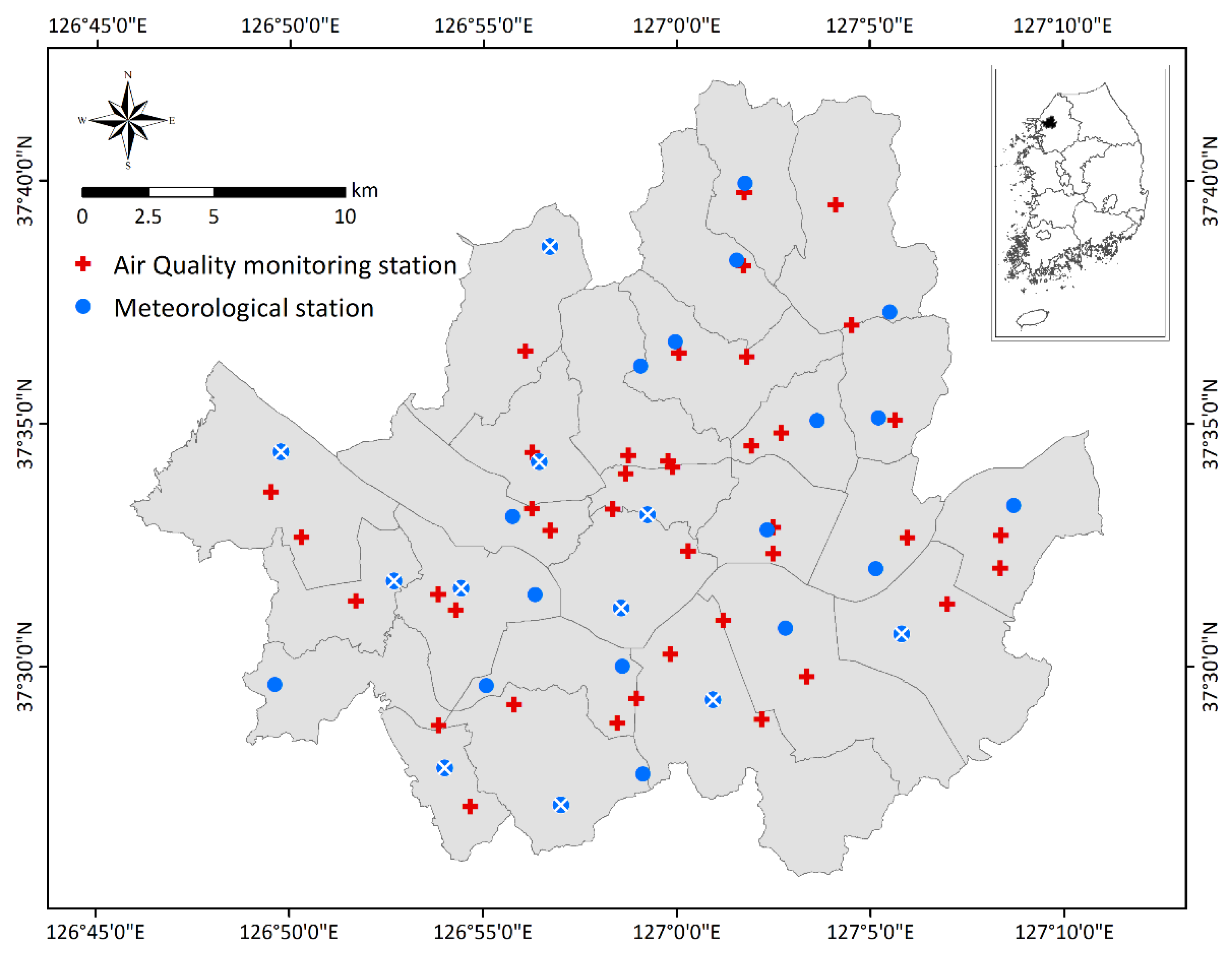
The spatial scope of this study was Seoul Metropolitan City, the capital of South Korea, and the temporal scope was from 2014 to 2016 (Figure 1). The population of Seoul during these years was approximately 10 million (15,865 persons/km2), with approximately 20% of the total population of South Korea living in Seoul, making it the fifth most populous metropolitan area worldwide [28,29]. The study area was characterized by a very high urban density, an abundance of high-rise buildings and apartments, mountainous terrain, and high vehicle densities in addition to a high population [30]. These features cause severe air pollution, leading to approximately 100,000 premature deaths annually, and social costs exceeding USD 10 billion [31,32].
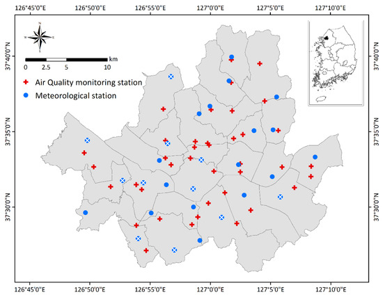
Figure 1.
Study area and spatial distribution of air quality monitoring and automatic weather stations. The X-marked blue circles were not used owing to missing observations.
In recent years, Seoul Metropolitan City has been striving to control and reduce local air pollutants through various measures. However, PM concentrations in Seoul are still higher than those in other large cities in developed countries, often exceeding the daily environmental control standard (100 μg/m2) [33,34,35]. Since 2004, when PM was first recorded in Seoul, the average number of days of yellow dust was approximately ten per year, while the number of days of yellow dust was highest at fifteen in 2015 [23]. In this study area, analysis of the effect of yellow dust as well as systematic air quality management are required through PM prediction.
2.2. Datasets
The data used in this study included PM10 air pollution data, emission data related to sulfurous acid gas (SO2), carbon monoxide (CO), ozone (O3), and nitrogen dioxide (NO2) as observed from the ground, and meteorological data such as temperature (Temp), rainfall (Rain), relative humidity (Humi), wind speed (Wind_S), wind degree (Wind_D), and yellow dust (Yellow). PM10 air pollution and emission data were collected from the Korea Environment Corporation (KECO). Meteorological data were collected from the National Climate Data Center (NCDC) of the Korea Meteorological Administration.
2.2.1. PM10 Air Pollution and Emission Data
We collected air pollution and emission data for three years (2014–2016) from AQMS in Seoul. The KECO has installed and operated air pollutant measurement equipment to identify the nationwide air pollution status, trends, and achievement of air quality standards [36]. In Seoul, a total of 39 AQMS were in operation during the study period, and they were mainly distributed in the central areas rather than the outer areas (Figure 1). AQMS provide hourly and daily average observations of PM10, PM2.5, sulfurous acid gas (SO2), carbon monoxide (CO), ozone (O3), and nitrogen dioxide (NO2) at each point. Among these observations, PM10 was selected for this study, as there was no PM2.5 observation value provided for 2014 during the study period. The daily average PM10 air pollution and emissions for the three years were collected and used (Table 1).

Table 1.
Data sources used in this study.
2.2.2. Meteorological Data
We used automatic weather station (AWS) data from the Korea Meteorological Administration to collect meteorological data for Seoul. AWS refers to ground observations conducted to prevent natural disasters caused by meteorological phenomena such as earthquakes, typhoons, floods, and droughts. To monitor local weather phenomena, AWS are installed at approximately 510 points across the country for automatic observation, with 28 stations in Seoul. These stations provide information on temperature, rainfall, relative humidity, wind speed, wind degree, and barometric pressure in min, h, d, months, and years [23]. In this study, hourly data for Temp, Rain, Humi, Wind_S, and Wind_D were collected and calculated as daily average values, excluding atmospheric pressure, for which there were no observed values during the study period (Table 1). However, at 11 stations, accounting for approximately 65% of the 28 stations located in the study area, humidity values were observed for at least three days and up to twelve days during the 1094 days of the study period (2014 to 2016). As a result, only data from 17 stations, excluding 11 out of 28 stations, were used.
In addition, we collected and used yellow dust data from the NCDC of the Korea Meteorological Administration as meteorological data. The Korea Meteorological Administration has installed and operated 30 stations across the country to observe yellow dust. Since 21 March 2003, each station has provided yellow dust concentrations every 5 min, and at an hourly rate. One yellow dust observation station was located in Seoul. In this study, the daily average value was calculated by collecting the hourly yellow dust concentration values measured at this station, which were then used as a representative value of the study area (Table 1).
2.3. Data Preprocessing and Matching
The air pollution and emission data used in this study were collected at each observation point by AQMS and meteorological data from the AWS. These data were collected from different institutions and had different observation points, as shown in Figure 1. Therefore, it was necessary to process these data and convert them into one dataset. Therefore, daily observation values of AWS observation points for the study area were generated as raster data using inverse distance weighting. The raster data for Temp, Rain, Humi, Wind_S, and Wind_D were generated with a spatial resolution of 30 m for each day. The generated raster data were overlapped with the AQMS data to extract cell values for each point. The total amount of data in the final dataset was 42,666, which was spatially matched to AQMS data, and days with missing values (1234) were excluded.
As a result, 27,587 data points for 2014 and 2015 were used as training data, and 13,845 data points for 2016 were used as verification data. The training data were used to generate the prediction model, whereas the validation data were applied to the generated prediction model to evaluate the prediction performance of the model. In this study, a grid search on hyperparameters with tenfold cross-validation was utilized to prevent model overfitting and enhance prediction accuracy while creating a predictive model. A tenfold cross-validation trains and evaluates the training data ten times by randomly dividing the training data into ten subsets. Each time, a different subset was selected and used to validate the model performance, and the remaining nine subsets were used for model training. Analysis was performed thrice, and the average of ten runs was used as the final result. Grid search is a method for manually adjusting hyperparameter values to determine the optimal combination.
2.4. Model Description
2.4.1. Gradient Boosting Machine
GBM is a representative boosting-based algorithm that sequentially generates trees in a way that compensates for the error of the decision tree generated in the previous step. Trees are gradually added to the previous ensemble tree model, and the model is trained in such a way that the next new tree is fitted with respect to the error of the previous model through gradient descent. Gradient descent is one of the simplest and most commonly used numerical optimization algorithms for determining the minimum value of the loss function along the gradient direction [37]. Therefore, the core of GBM uses the negative gradient of the loss function as the residual approximation in the lifting tree algorithm and minimizes the loss function by gradually reducing the residual value [16]. For the GBM model, the “GBM” package of the R program was used; the optimal values of the hyperparameters are shown in Table A1 (Appendix A).
2.4.2. Extreme Gradient Boosting
GBM has many advantages, such as the ability to handle mixed types of features, the function of feature combination, easier interpretability, faster running speed, and lower memory consumption [38]. However, GBM often results in overfitting, and various algorithms have been developed to solve this. Extreme gradient boosting (XGBoost), which is an efficient implementation of GBM, is a scalable end-to-end tree boosting system. Compared to GBM, XGBoost avoids overfitting by using regularized boosting and parallel processing [39]. In addition, this algorithm can overcome the limitations of computing speed and accuracy, requires less training and time for prediction, and supports various objective functions including classification, regression, and ranking [40]. XGBoost was built using the “xgboost” package of the R program; the optimal values of the hyperparameters are shown in Table A2.
2.4.3. Light Gradient Boost Machine
LightGBM is a gradient promotion framework based on decision trees developed by Microsoft for tasks such as sorting, classification, and regression, and which can model complex nonlinear functions [21]. XGBoost employs the exact voracious algorithm, whereas LightGBM employs a histogram-based decision-tree algorithm. Therefore, the leaf-by-leaf growth strategy with deep constraints, which speeds up the training process to reduce memory consumption and training time, was selected [41]. LightGBM provides advantages such as performance improvement, faster training speed, lower memory consumption, higher effect accuracy, and fast processing of massive data. In addition, this algorithm supports category features without 0–1 encoding, and allows for efficient parallel training [8,21]. The LightGBM model was constructed using the “lightgbm” package of the R program; the optimal values of the hyperparameters are shown in Table A3.
2.5. Model Validation
In this study, the coefficient of determination (R2), root mean square error (RMSE), mean absolute error (MAE), and mean absolute percentage error (MAPE) were used to evaluate model performance. These metrics are commonly used to evaluate the accuracy of regression models and indicate the degree of error between the predicted and observed values.
R2 is used to evaluate the explanatory power of the independent variables with respect to the dependent variables (Equation (1)). R2 ranges from 0 to 1, and the higher the accuracy of the model, the closer it is to 1. However, as the number of independent variables and data increases, the value of R2 tends to increase regardless of the prediction performance of the model. To compensate for this problem, the adjusted R2 is indicated by additionally considering the size of the data and the number of independent variables. In this study, the adjusted R2 was calculated using Equation (2). The MSE is the average of the sum of the squares of the difference (error) between the actual and predicted values. If the sum of the squared errors is too large, the MSE may also become too large. To compensate for this, the MSE is rooted, yielding the RMSE. The RMSE is calculated using Equation (3), and is used synonymously with a standard deviation. As the RMSE depends on the scale, it is called a scale-dependent error. Because the MAE is calculated by converting the error into an absolute value and averaging it (Equation (4)), it reflects the size of the error as is. The MAPE is the MAE converted into a percentage (Equation (5)), and is called a percentage error. The MAPE is more robust than the RMSE and MSE against outliers, and is easy to understand because it ranges between 0% and 100%. Lower values of the RMSE, MSE, and MAPE indicate higher accuracy.
3. Results and Discussion
3.1. Effect of Input Variables on PM10 Prediction
In this study, a PM10 prediction model was constructed using the GBM, XGB, and LightGBM algorithms with a total of ten independent variables as input values. When constructing prediction models, the algorithm used in this study provides feature importance values for the input factors. Feature importance is a score representing the importance (contribution) of each independent variable in PM10 prediction. The importance of any variable is calculated by the amount of increase in the performance measure because of that variable in a decision tree. The purity (Gini index) was used as the performance measure. Eventually, the importance of the variable is determined by averaging the importance of all decision trees.
Table 2 shows the rankings of the calculated importance for the ten independent variables used in this study; the higher the ranking (the smaller the number), the higher the importance. Among the ten independent variables, Yellow (yellow dust) had the highest importance. This suggests that Yellow plays a dominant role in the three models used in this study. However, except for Yellow, the significance of each variable varied significantly among the models. Among the top five factors, the variables with high importance in all three models were Yellow, Temp (temperature), and NO2 (NO2). However, in the GBM model, Wind_D (wind degree) and SO2 were more important than in the other models. CO and Humi (relative humidity) were highly important in the XGBoost model, and Humi, and Rain (rainfall) were important in the LightGBM model.
Table 2.
Relative importance of independent PM10-related variables for each model.
The sources of PM emissions in Korea may be classified into two categories, internal and external sources. The primary internal sources include thermal power plants, construction machinery, automobile exhaust gas, scattering dust, and air conditioning; the primary external sources include industrial dust from inland industrial areas in China and yellow dust from the Gobi Desert. The proportion of foreign influence is generally approximately 50% per year, which may be up to approximately 80% depending on the season and weather conditions [31]. This indicates that yellow dust is one of the main factors affecting domestic air quality. However, there is only one yellow dust observatory in the study area, and it is difficult to accurately reflect the amount of PM moving long distances from China. In particular, in the results of our analysis, the contribution of the Yellow variable for each model was approximately 90%, with a significant effect even with a slight change in the observed value. To reflect the effect of yellow dust on PM in the future, a review of various aspects is necessary.
Temperature and humidity can influence the rate of decrease in PM by influencing the movement and dispersion of PM on a micro-spatiotemporal scale [42]. Upon analyzing the correlation between changes in weather conditions and PM in the metropolitan area, the National Academy of Environmental Sciences reported a correlation between PM concentrations and temperature and humidity [43]. This is in line with the results of this study, where temperature and humidity contributed significantly to generating a PM prediction model. Among the gaseous pollutants used in this study, CO and NO2 were of relatively high importance. Generally, PM10 was highly correlated with CO and NOx in major urban areas of South Korea. In particular, a strong correlation was observed between PM10 and cities with high population density, suggesting their correlation with traffic emissions [44].
3.2. Evaluation of Model Performance
3.2.1. Performance Comparison between Models
Figure 2 shows the accuracy of the three PM10 prediction models built in this study. Model accuracy measures how effectively the predictive model developed in this study matches the input data. In order to analyze model accuracy, the accuracy between the predicted and observed values was calculated by inputting the training data into the built prediction model. All three models used in this study had an adjusted R2 value of 95% or higher, which indicates that all models represented the characteristics of the independent variables used in this study. In particular, for the LightGBM model adopted in this study, the adjusted R2, RMSE, MAE, and MAPE were 0.96, 6.655 μg/m2, 4.535 μg/m2, and 11%, respectively. These values were similar to those of the GBM model, indicating a relatively low accuracy compared to the XGB model. Overall, the predicted and observed values of PM10 were in good agreement.
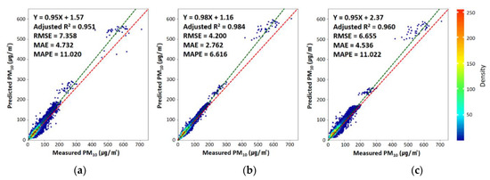
Figure 2.
Density scatter plots of model fitting for (a) gradient boosting machine, (b) extreme gradient boosting, and (c) light gradient boosting machine from 2014 to 2015 (N = 27,587). The red and green dotted lines are the 1:1 line and linear regression line, respectively. The performance of each model was calculated using statistical metrics such as the correlation of determination (Adjusted R2), the root mean square error (RMSE), the mean absolute error (MAE), and the mean absolute percentage error (MAPE), as noted at the top left of each panel.
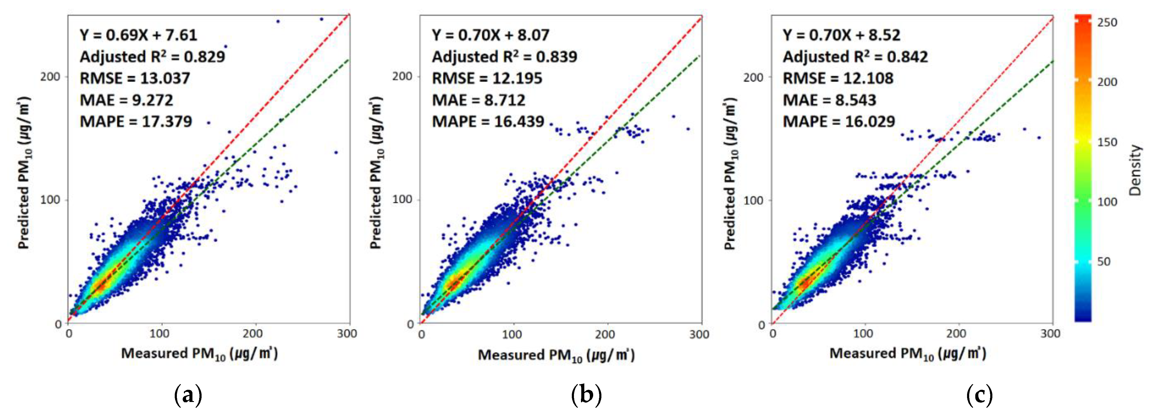
Figure 3 shows the prediction accuracies of the three models. The prediction accuracy represents the prediction performance when new data are applied to the built prediction model. To analyze prediction accuracy, the accuracy levels of the predicted and observed values were calculated by applying a test dataset that was not used when constructing the prediction model. The prediction accuracy levels of all three models used in this study in terms of the adjusted R2 were approximately 12–15% lower than the model accuracy. The adjusted R2, RMSE, MAE, and MAPE of LightGBM were 0.84, 12.108 μg/m2, 8.543 μg/m2, and 16%, respectively. Unlike the model accuracy, the LightGBM model had the highest prediction performance among the three models used in this study. XGB yielded a slightly lower level of accuracy than LightGBM, and GBM exhibited the lowest level of accuracy.

Figure 3.
Density scatter plots of model prediction power for (a) gradient boosting machine, (b) extreme gradient boosting, and (c) light gradient boosting machine in 2016 (N = 13,845). The red and green dotted lines are the 1:1 line and linear regression line, respectively. The performance of each model is calculated using statistical metrics such as the correlation of determination (Adjusted R2), the root mean square error (RMSE), the mean absolute error (MAE), and the mean absolute percentage error (MAPE), as noted at the top left of each panel.
3.2.2. Model Selection on PM10 Prediction
Among the models used in this study, the XGB model was found to have excellent performance owing to its high model and prediction accuracies. However, the model training time was the longest, 41.89 s. In addition, the prediction performance was rather low compared to the high model accuracy. Conversely, the LightGBM model yielded the fastest execution time (1.36 s) as well as the highest prediction accuracy. Boosting models require the optimization of a relatively large number of hyperparameters. Optimizing the hyperparameters and creating training models takes a long time. However, the use of the LightGBM model is expected to allow for the fast construction of a prediction model and generation of prediction results when processing a large amount of data. As this model appears to have a relatively high prediction accuracy compared to other models, it evidently contributes to solving the overfitting problem to a certain extent. Therefore, the LightGBM model was selected as the optimal model for predicting PM10 concentrations in this study, and its prediction accuracy was further examined in terms of space and time.
3.3. Performance Evaluation of the LightGBM Model
3.3.1. Site-Scale Model Performance
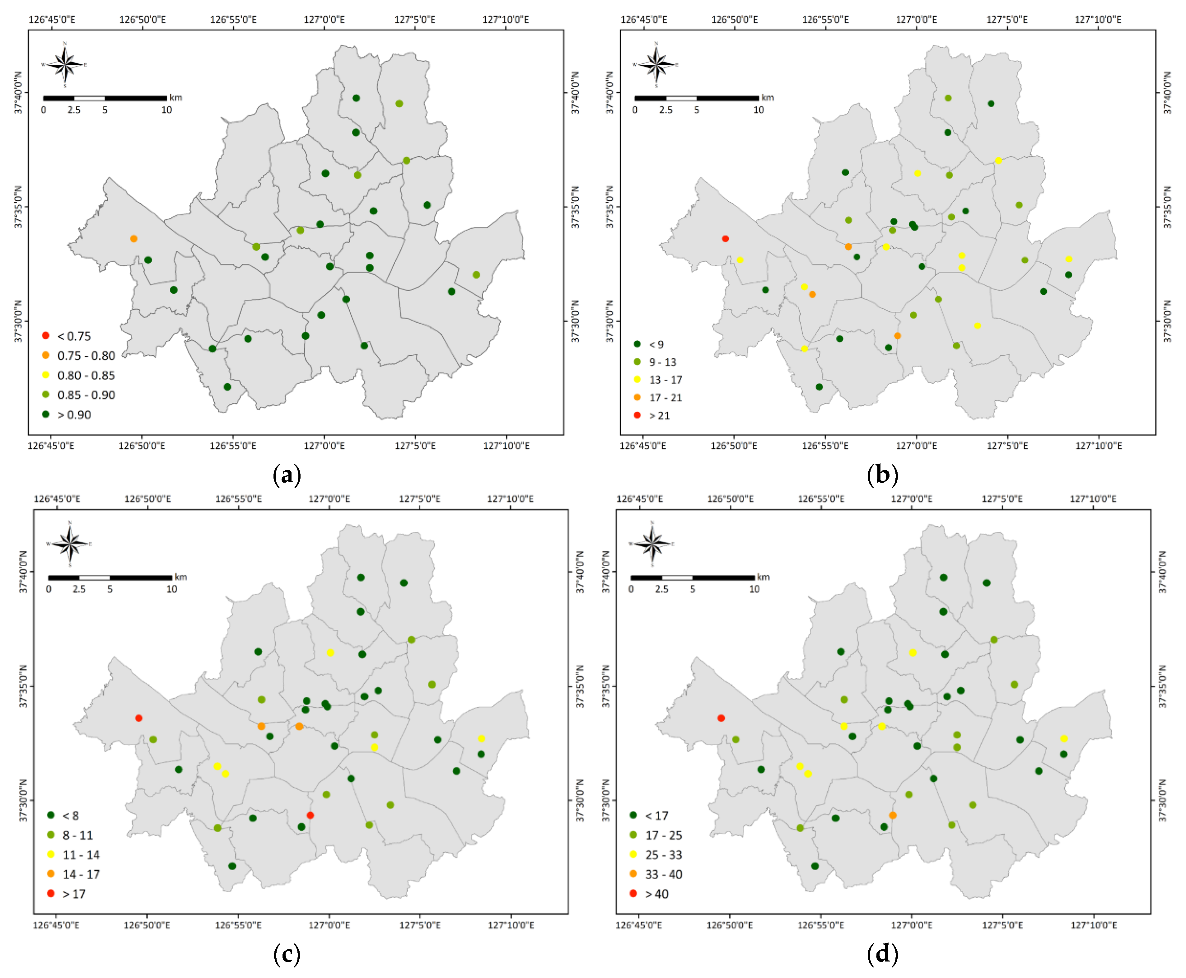
We evaluated the prediction accuracy of the LightGBM model based on 39 AQMSs located in Seoul Metropolitan City in order to evaluate its spatial performance. Figure 4 shows the average annual prediction performance for each station using a total of four statistical metrics: adjusted R2, RMSE, MAE, and MAPE. For most stations, the adjusted R2 value was 0.85 or higher, and the average value was 0.92. The RMSE ranged from 5.183 to 24.786 μg/m2, and was as high as 20 μg/m2 in three out of a total of 39 stations. Compared to the RMSE, the MAE was relatively low, ranging from 3.910 to 20.552 μg/m2 (average 8.523 μg/m2). The MAPE had a similar spatial distribution to the RMSE and MAE, with a mean value of 19%. Overall, the predicted and ground-observed PM10 concentrations were highly consistent.
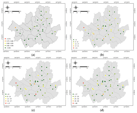
Figure 4.
Spatial distributions of site-scale performance for each PM10 monitoring station using (a) correlation of determination (Adjusted R2), (b) the root mean square error (RMSE), (c) the mean absolute error (MAE), and (d) the mean absolute percentage error (MAPE). All statistical metrics were reclassified and mapped by a five-class equal interval classification scheme using ArcGIS.
However, the prediction accuracy was low at some stations located near the southwest of the study area. In particular, the Gonghang-ro observation station (111213), located in the westernmost part of the study area, yielded the lowest values for the adjusted R2, RMSE, MAE, and MAPE at 0.76, 24.786 μg/m2, 20.552 μg/m2, and 48%, respectively. This result is attributed to several factors. First, the meteorological factors used in this study were automatically observed data from the AWS located in the study area. In Figure 1, at 11 stations, accounting for approximately 65% of the 28 stations located in the study area, humidity data were collected only for 3–12 days during the 1094 days of the study period (2014 to 2016). These 11 stations were excluded from this study because of missing observation values. The relatively low prediction performance at certain AQMS may have been due to the omission of AWS located near the stations resulting in a limited reflection of climate characteristics.
Second, a distribution map was created by counting emission establishments based on the 2016 classification in the Environmental Statistics Yearbook published by the Ministry of Environment. An emission establishment refers to a business that has installed emission facilities that emit air pollutants among substances present in the atmosphere. Generally, there were relatively more emission establishments in the southwestern region of the study area. Emission establishments appeared to have a certain impact on PM concentrations. Identifying related factors in the future and reflecting them when constructing the model seems necessary.
Lastly, there is an airport and a port located near Gonghang-ro observation station which yielded the lowest prediction accuracy in the study area. Previous studies have reported that proximity to airports or air cargo facilities was strongly correlated with PM10 concentrations [45,46]. Aircraft departure activities at airports have been reported to significantly contribute to changes in PM concentrations [47], and airport daily contribution to PM concentrations was approximately 1.4 times greater than that of nearby highways [46]. According to a study by Broome et al., 2016 [48], approximately 1.9% of the region-wide annual average population weighted-mean concentration of all natural and human-made PM2.5 was attributable to ship exhausts, and this value can be as high as 9.4% in suburbs close to ports. Clearly, proximity to airports and ports affects the PM concentration.
3.3.2. Daily and Seasonal Validation
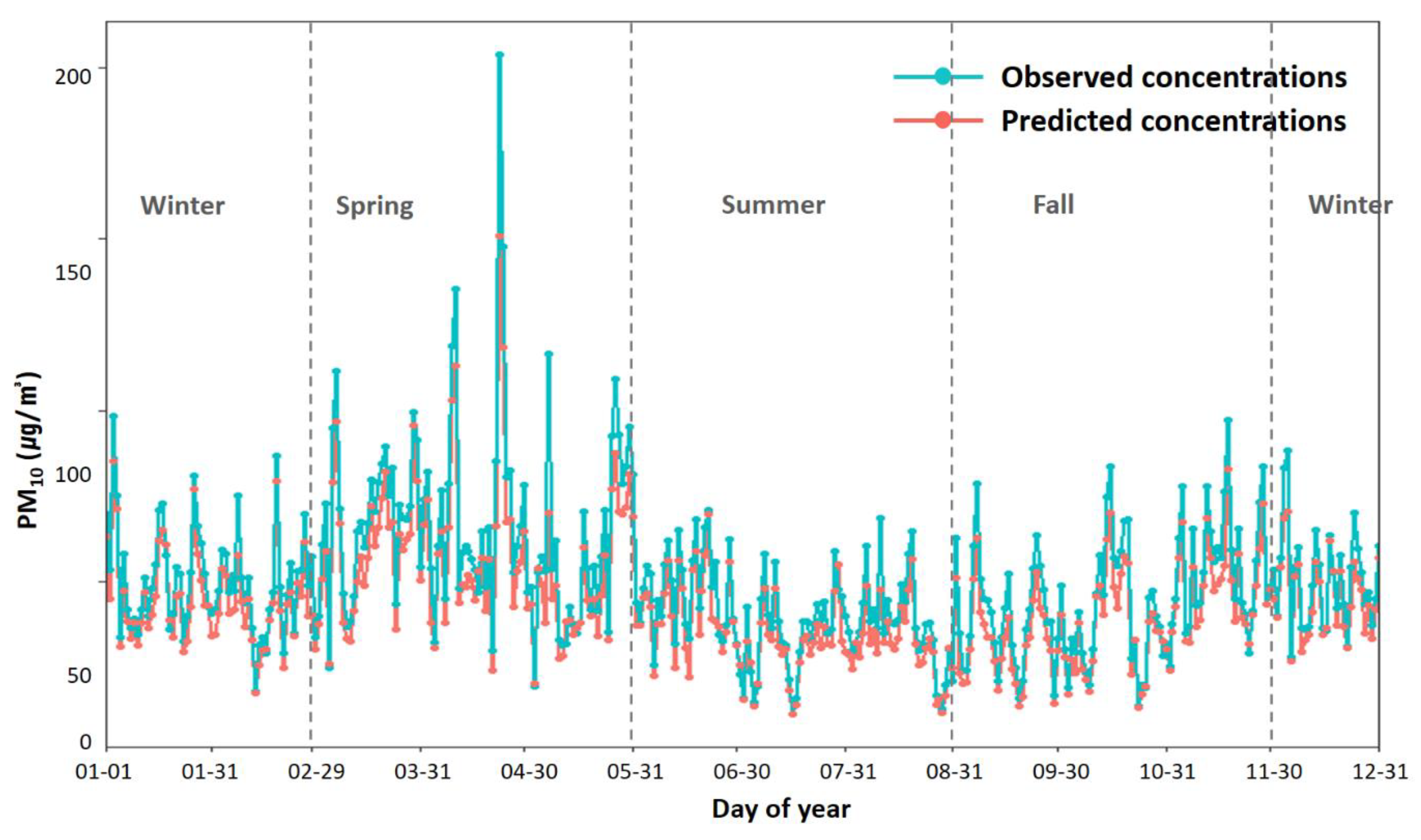
Figure 5 shows a comparison of the daily distribution of PM10 concentrations by calculating the daily average value in order to elucidate the trends of the predicted and observed values. The predicted daily average concentrations ranged from 11.407 to 150.700 μg/m2; however, the daily average concentrations of the observed values ranged from 11.257 to 203.922 μg/m2, with a rather high maximum. The average predicted value was 43.687 μg/m2, and the average observed value was rather high, at 50.435 μg/m2. Overall, the predicted values showed a trend that was similar to that of the observed values. However, the values predicted by the LightGBM model were generally slightly underestimated compared to the observed values. In particular, the observed and predicted values differed slightly when the PM10 concentration was low in 2016; however, the difference between these values increased as the concentration of PM10 increased. The observed PM10 concentrations throughout the year were very high, exceeding 100 μg/m2 for seven days during spring (March–May); in particular, the observed value on 23 April was the highest (203.922 μg/m2), and its difference from the predicted value (150.700 μg/m2) was also the largest, at 53.222 μg/m2.

Figure 5.
Time-scale performance of the daily mean distributions of estimated PM10 concentrations in 2016. The daily mean distributions of estimated and observed PM10 concentrations were compared.
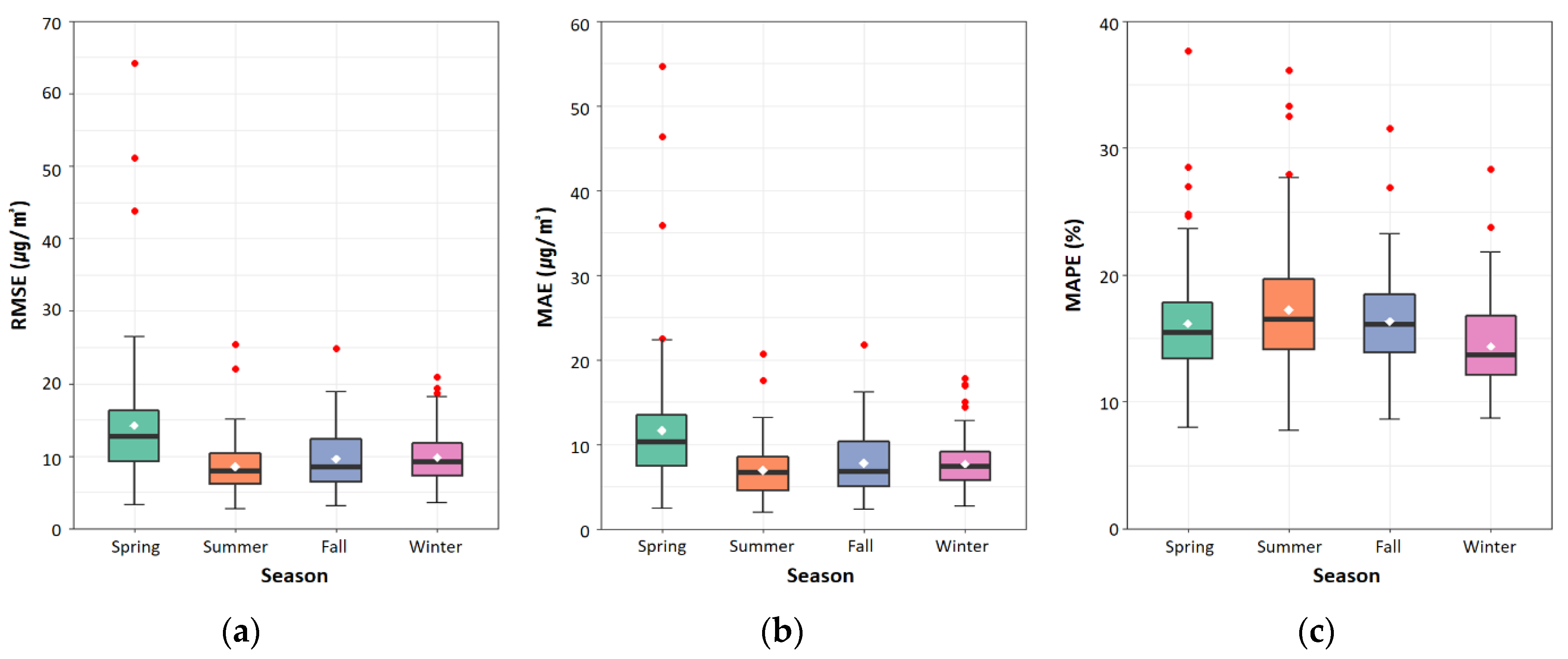
This study evaluated the daily accuracy for the entire study area to evaluate the time-scale performance of the LightGBM model. Figure 6 shows the boxplots based on which we examined the seasonal distribution of the calculated daily accuracy. The average RMSE, MAE, and MAPE values during spring showed the lowest accuracy, at 14.244 μg/m2, 11.666 μg/m2, and 20.07%, respectively. In contrast, the average RMSE, MAE, and MAPE values during summer showed the highest accuracies of 8.541 μg/m2, 6.958 μg/m2, and 20.47%, respectively. In South Korea, a high concentration of PM accompanied by yellow dust is likely to be observed in spring, and the PM concentration tends to decrease in summer and autumn. Therefore, the prediction accuracy of PM10 will seemingly be improved using more variables reflecting seasonal characteristics. However, the meteorological factors used in this study were measured using automatic observation equipment by the Korea Meteorological Administration, providing only a limited number of parameters. In the future, use of the numerical forecast model provided by the Korea Meteorological Administration will allow for the reflection of more diverse meteorological variables. Among the numerical forecasting models operated by the Korea Meteorological Administration, the Local Assimilation and Prediction System (LDAPS) is a Korean model created by regionally optimizing the unified model of the UK Met Office. LDAPS provides information on 78 meteorological variables by performing short-term forecasts throughout the Korean Peninsula, with a horizontal resolution of 1.5 km and a vertical resolution of approximately 40 km [23].
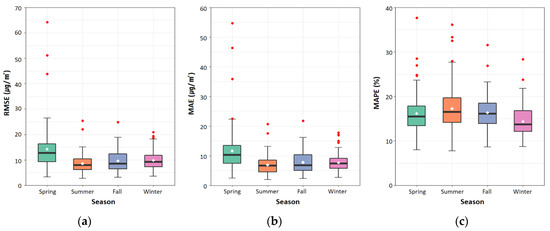
Figure 6.
Time-scale performance regarding seasonal distributions of estimated PM10 concentrations in 2016. The seasonal distributions were plotted as boxplots of (a) the root mean square error (RMSE), (b) the mean absolute error (MAE), and (c) the mean absolute percentage error (MAPE) for estimated and observed PM10 concentrations. Here, the white dot denotes the seasonal mean value of each statistical metric.
4. Conclusions
We aimed to create a PM prediction model using GBM, XGBoost, and LightGBM for Seoul Metropolitan City in South Korea. The PM prediction model for each algorithm was analyzed and compared in terms of accuracy using statistical metrics such as R2, RMSE, MAE, and MAPE. The analysis showed that the LightGBM model outperformed the GBM and XGBoost models, with a relatively high prediction accuracy, fast execution time, and reduced overfitting problems. Accordingly, the LightGBM model was identified as suitable for predicting PM in the study area, and the spatiotemporal distribution characteristics of the results predicted by the LightGBM model were examined. The LightGBM model showed low spatial prediction accuracy near the southwest part of the study area. In terms of time, the predicted and observed values showed a similar trend; however, at high PM concentrations, the difference between the observed and predicted values increased. These results suggest that the prediction performance of the LightGBM model can be improved by considering various variables that reflect spatial and seasonal characteristics. The results of this study will provide more reliable PM concentration values at the regional level for areas with no AQMS. They will also be useful as supporting data to establish measures for managing, preventing, and mitigating air pollution in the study area.
Author Contributions
S.P. wrote the paper and analyzed the data; S.S., J.B. and D.L. collected the data and performed preprocessing; J.-J.K. reviewed the paper in terms of atmospheric science; J.K. suggested the idea for the study. All authors have read and agreed to the published version of the manuscript.
Funding
This research was funded by a grant of the National Research Foundation of Korea (NRF) funded by the Ministry of Education and the Ministry of Science and ICT (2019M3E7A1113103, 2020R1A2B5B02002198, 2020R1I1A1A01075106).
Institutional Review Board Statement
Not applicable.
Informed Consent Statement
Not applicable.
Acknowledgments
This research was supported by a grant of the National Research Foundation of Korea (NRF) funded by the Ministry of Education and the Ministry of Science and ICT (2019M3E7A1113103, 2020R1A2B5B02002198, 2020R1I1A1A01075106).
Conflicts of Interest
The authors declare no conflict of interest.
Appendix A
Table A1.
Gradient boosting machine parameters.
Table A1.
Gradient boosting machine parameters.
| Attribute | Explain | Parameter |
|---|---|---|
| shrinkage | Learning rate | 0.01 |
| interaction.depth | Maximum depth of each tree | 4 |
| n.minobsinnode | Minimum number of observations in trees’ terminal nodes | 92 |
| bag.fraction | Fraction of the training set observations randomly selected | 0.6 |
| train.fraction | Proportion of samples used for training and testing | 0.7 |
Table A2.
Extreme gradient boosting parameters.
Table A2.
Extreme gradient boosting parameters.
| Attribute | Explain | Parameter |
|---|---|---|
| eta | Learning rate | 0.01 |
| max_depth | Maximum depth of a tree | 14 |
| min_child_weight | Minimum sum of instance weight (hessian) | 17 |
| subsample | Subsample ratio of the training instance | 0.8 |
| colsample_bytree | Subsample ratio of columns when constructing each tree | 1.0 |
| lambda | L2 Regularization term on weights | 11 |
| alpha | L1 Regularization term on weights | 27 |
Table A3.
Parameters of light gradient boosting machine.
Table A3.
Parameters of light gradient boosting machine.
| Attribute | Explain | Parameter |
|---|---|---|
| learning_rate | Learning rate | 0.01 |
| max_depth | Maximum depth of a tree | 6 |
| num_leaves | Maximum number of leaves in one tree | 19 |
| min_data_in_leaf | Minimum number of observations in one leaf | 11 |
| bagging_fraction | Subsample ratio of the training instance | 0.8 |
| bagging_freq | Frequency for bagging | 3 |
| feature_fraction | Subsample ratio of columns when constructing each tree | 1.0 |
| lambda_l1 | L1 regularization term on weights | 0.9 |
| lambda_l2 | L2 regularization term on weights | 0.4 |
References
- Cohen, A.J.; Anderson, H.R.; Ostro, B.; Pandey, K.D.; Krzyzanowski, M.; Künzli, N.; Gutschmidt, K.; Pope, A.; Romieu, I.; Samet, J.M.; et al. The Global Burden of Disease Due to Outdoor Air Pollution. J. Toxicol. Environ. Health Part A 2005, 68, 1301–1307. [Google Scholar] [CrossRef]
- Shtein, A.; Kloog, I.; Schwartz, J.; Silibello, C.; Michelozzi, P.; Gariazzo, C.; Viegi, G.; Forastiere, F.; Karnieli, A.; Just, A.C.; et al. Estimating Daily PM2.5 and PM10 over Italy Using an Ensemble Model. Environ. Sci. Technol. 2020, 54, 120–128. [Google Scholar] [CrossRef] [PubMed]
- International Agency for Research on Cancer (IARC). Outdoor Air Pollution a Leading Environmental Cause of Cancer Deaths; International Agency for Research on Cancer: Lyon, France, 2013. [Google Scholar]
- Allen, M.; Antwi-Agyei, P.; Aragon-Durand, F.; Babiker, M.; Bertoldi, P.; Bind, M.; Zickfeld, K. Technical Summary: Global Warming of 1.5 °C. An IPCC Special Report on the Impacts of Global Warming of 1.5 °C above Pre-Industrial Levels and Related Global Greenhouse Gas Emission Pathways, in the Context of Strengthening the Global Response to the Threat of Climate Change, Sustainable Development, and Efforts to Eradicate Poverty; IPCC: Geneva, Switzerland, 2019. [Google Scholar]
- Hwang, I.C.; Kim, K.U.; Baek, J.R.; Son, W.I. Long-Term Strategy and Sectoral Approaches of Seoul for Achieving Carbon Neutrality by 2050; The Seoul Institute: Seoul, Korea, 2020; pp. 1–162. [Google Scholar]
- Cho, M.; Choi, Y.-S.; Kim, H.-R.; Yoo, C.; Lee, S.-S. Cold-season atmospheric conditions associated with sudden changes in PM10 concentration over Seoul, Korea. Atmos. Pollut. Res. 2021, 12, 101041. [Google Scholar] [CrossRef]
- Ministry of Environment Website. Available online: https://www.me.go.kr/cleanair (accessed on 20 June 2021).
- Zhang, Y.; Zhang, R.; Ma, Q.; Wang, Y.; Wang, Q.; Huang, Z.; Huang, L. A feature selection and multi-model fusion-based approach of predicting air quality. ISA Trans. 2020, 100, 210–220. [Google Scholar] [CrossRef] [PubMed]
- Konovalov, I.; Beekmann, M.; Meleux, F.; Dutot, A.; Foret, G. Combining deterministic and statistical approaches for PM10 forecasting in Europe. Atmos. Environ. 2009, 43, 6425–6434. [Google Scholar] [CrossRef]
- Song, Y.; Qin, S.; Qu, J.; Liu, F. The forecasting research of early warning systems for atmospheric pollutants: A case in Yangtze River Delta region. Atmos. Environ. 2015, 118, 58–69. [Google Scholar] [CrossRef]
- Bozdağ, A.; Dokuz, Y.; Gökçek, Ö.B. Spatial prediction of PM10 concentration using machine learning algorithms in Ankara, Turkey. Environ. Pollut. 2020, 263, 114635. [Google Scholar] [CrossRef]
- Chen, G.; Li, S.; Knibbs, L.D.; Hamm, N.A.S.; Cao, W.; Li, T.; Guo, J.; Ren, H.; Abramson, M.J.; Guo, Y. A machine learning method to estimate PM2.5 concentrations across China with remote sensing, meteorological and land use information. Sci. Total Environ. 2018, 636, 52–60. [Google Scholar] [CrossRef]
- Chen, G.; Wang, Y.; Li, S.; Cao, W.; Ren, H.; Knibbs, L.; Abramson, M.J.; Guo, Y. Spatiotemporal patterns of PM10 concentrations over China during 2005–2016: A satellite-based estimation using the random forests approach. Environ. Pollut. 2018, 242, 605–613. [Google Scholar] [CrossRef] [PubMed]
- Di, Q.; Amini, H.; Shi, L.; Kloog, I.; Silvern, R.; Kelly, J.; Sabath, M.B.; Choirat, C.; Koutrakis, P.; Lyapustin, A.; et al. An ensemble-based model of PM2.5 concentration across the contiguous United States with high spatiotemporal resolution. Environ. Int. 2019, 130, 104909. [Google Scholar] [CrossRef] [PubMed]
- Guo, B.; Zhang, D.; Pei, L.; Su, Y.; Wang, X.; Bian, Y.; Zhang, D.; Yao, W.; Zhou, Z.; Guo, L. Estimating PM2.5 concentrations via random forest method using satellite, auxiliary, and ground-level station dataset at multiple temporal scales across China in 2017. Sci. Total Environ. 2021, 778, 146288. [Google Scholar] [CrossRef] [PubMed]
- Zhang, T.; He, W.; Zheng, H.; Cui, Y.; Song, H.; Fu, S. Satellite-based ground PM2.5 estimation using a gradient boosting decision tree. Chemosphere 2021, 268, 128801. [Google Scholar] [CrossRef] [PubMed]
- Yazdi, M.D.; Kuang, Z.; Dimakopoulou, K.; Barratt, B.; Suel, E.; Amini, H.; Lyapustin, A.; Katsouyanni, K.; Schwartz, J. Predicting Fine Particulate Matter (PM2.5) in the Greater London Area: An Ensemble Approach using Machine Learning Methods. Remote Sens. 2020, 12, 914. [Google Scholar] [CrossRef] [Green Version]
- Joharestani, M.Z.; Cao, C.; Ni, X.; Bashir, B.; Talebiesfandarani, S. PM2.5 Prediction Based on Random Forest, XGBoost, and Deep Learning Using Multisource Remote Sensing Data. Atmosphere 2019, 10, 373. [Google Scholar] [CrossRef] [Green Version]
- Li, Z.; Yim, S.H.-L.; Ho, K.-F. High temporal resolution prediction of street-level PM 2.5 and NOx concentrations using machine learning approach. J. Clean. Prod. 2020, 268, 121975. [Google Scholar] [CrossRef]
- Wei, J.; Li, Z.; Pinker, R.T.; Wang, J.; Sun, L.; Xue, W.; Li, R.; Cribb, M. Himawari-8-derived diurnal variations in ground-level PM2.5 pollution across China using the fast space-time Light Gradient Boosting Machine (LightGBM). Atmos. Chem. Phys. Discuss. 2021, 21, 7863–7880. [Google Scholar] [CrossRef]
- Zeng, Z.; Gui, K.; Wang, Z.; Luo, M.; Geng, H.; Ge, E.; An, J.; Song, X.; Ning, G.; Zhai, S.; et al. Estimating hourly surface PM2.5 concentrations across China from high-density meteorological observations by machine learning. Atmos. Res. 2021, 254, 105516. [Google Scholar] [CrossRef]
- Zhong, J.; Zhang, X.; Gui, K.; Wang, Y.; Che, H.; Shen, X.; Zhang, L.; Zhang, Y.; Sun, J.; Zhang, W. Robust prediction of hourly PM2.5 from meteorological data using LightGBM. Natl. Sci. Rev. 2021, 8, 1–12. [Google Scholar] [CrossRef]
- Korea Meteorological Administration. Meteorological Agency. Available online: https://data.kma.go.kr (accessed on 20 June 2021).
- Lee, B.-K.; Jun, N.-Y.; Lee, H.K. Comparison of particulate matter characteristics before, during, and after Asian dust events in Incheon and Ulsan, Korea. Atmos. Environ. 2004, 38, 1535–1545. [Google Scholar] [CrossRef]
- Kim, K.-H.; Kim, M.-Y. The effects of Asian Dust on particulate matter fractionation in Seoul, Korea during spring 2001. Chemosphere 2003, 51, 707–721. [Google Scholar] [CrossRef]
- Choi, H.; Lee, M.S. Atmospheric boundary layer influenced upon hourly PM10, PM2.5, PM1 concentrations and their correlations at Gangneung city before and after yellow dust transportation from Gobi Desert. J. Clim. Res. 2012, 7, 30–54. [Google Scholar]
- Choi, J.-E.; Lee, H.; Song, J. Forecasting daily PM10concentrations in Seoul using various data mining techniques. Commun. Stat. Appl. Methods 2018, 25, 199–215. [Google Scholar] [CrossRef] [Green Version]
- Statistics Korea. Korean Statistical Information Service. Available online: http://kostat.go.kr/ (accessed on 17 June 2021).
- Lim, C.C.; Kim, H.; Vilcassim, M.J.R.; Thurston, G.D.; Gordon, T.; Chen, L.C.; Lee, K.; Heimbinder, M.; Kim, S.-Y. Mapping urban air quality using mobile sampling with low-cost sensors and machine learning in Seoul, South Korea. Environ. Int. 2019, 131, 105022. [Google Scholar] [CrossRef] [PubMed]
- Kim, H.-S.; Huh, J.-B.; Hopke, P.K.; Holsen, T.M.; Yi, S.-M. Characteristics of the major chemical constituents of PM 2.5 and smog events in Seoul, Korea in 2003 and 2004. Atmos. Environ. 2007, 41, 6762–6770. [Google Scholar] [CrossRef]
- Lee, S.; Ho, C.-H.; Choi, Y.-S. High-PM10 concentration episodes in Seoul, Korea: Background sources and related meteorological conditions. Atmos. Environ. 2011, 45, 7240–7247. [Google Scholar] [CrossRef]
- Gyeonggi Research Institute. Estimating Social Costs of Air Pollutions and Developing Emission Control Strategies for Kyonggi-Do; Gyeonggi Research Institute: Suwon, Korea, 2003. [Google Scholar]
- Kim, K.-H.; Shon, Z.-H. Long-term changes in PM10 levels in urban air in relation with air quality control efforts. Atmos. Environ. 2011, 45, 3309–3317. [Google Scholar] [CrossRef]
- Korean Ministry of Environment. Annual Report of Ambient Air Quality in Korea; Korean Ministry of Environment: Seoul, Korea, 2009; p. 121. [Google Scholar]
- Lee, S.; Ho, C.-H.; Lee, Y.G.; Choi, H.-J.; Song, C.-K. Influence of transboundary air pollutants from China on the high-PM10 episode in Seoul, Korea for the period October 16–20, 2008. Atmos. Environ. 2013, 77, 430–439. [Google Scholar] [CrossRef]
- Korea Environment Corporation Website. Available online: https://airkorea.or.kr (accessed on 20 June 2021).
- Wang, J.; Li, P.; Ran, R.; Che, Y.; Zhou, Y. A Short-Term Photovoltaic Power Prediction Model Based on the Gradient Boost Decision Tree. Appl. Sci. 2018, 8, 689. [Google Scholar] [CrossRef] [Green Version]
- Luo, Z.; Huang, F.; Liu, H. PM2.5 concentration estimation using convolutional neural network and gradient boosting machine. J. Environ. Sci. 2020, 98, 85–93. [Google Scholar] [CrossRef]
- Chen, T.; Guestrin, C. Xgboost: A scalable tree boosting system. In Proceedings of the 22nd ACM SIGKDD International Conference on Knowledge Discovery and Data Mining, San Francisco, CA, USA, 13–17 August 2016; pp. 785–794. [Google Scholar]
- Gui, K.; Che, H.; Zeng, Z.; Wang, Y.; Zhai, S.; Wang, Z.; Luo, M.; Zhang, L.; Liao, T.; Zhao, H.; et al. Construction of a virtual PM2.5 observation network in China based on high-density surface meteorological observations using the Extreme Gradient Boosting model. Environ. Int. 2020, 141, 105801. [Google Scholar] [CrossRef]
- Ke, G.; Meng, Q.; Finley, T.; Wang, T.; Chen, W.; Ma, W.; Ye, Q.; Liu, T.Y. Lightgbm: A highly efficient gradient boosting decision tree. Adv. Neural Inf. Process. Syst. 2017, 30, 3146–3154. [Google Scholar]
- Yoo, S.-Y.; Kim, T.; Ham, S.; Choi, S.; Park, C.-R. Importance of Urban Green at Reduction of Particulate Matters in Sihwa Industrial Complex, Korea. Sustainability 2020, 12, 7647. [Google Scholar] [CrossRef]
- National Institute of Environmental Research. Analysis of Pollution Caused by Particulate Matter in the Metropolitan Area and Prediction Failures—Final Report; Ewha University-Industry Collaboration Foundation (EUICF): Seoul, Korea, 2007. [Google Scholar]
- Sharma, A.P.; Kim, K.-H.; Ahn, J.; Shon, Z.; Sohn, J.; Lee, J.; Ma, C.; Brown, R. Ambient particulate matter (PM10) concentrations in major urban areas of Korea during 1996–2010. Atmos. Pollut. Res. 2014, 5, 161–169. [Google Scholar] [CrossRef] [Green Version]
- Amini, H.; Taghavi, M.; Henderson, S.B.; Naddafi, K.; Nabizadeh, R.; Yunesian, M. Land use regression models to estimate the annual and seasonal spatial variability of sulfur dioxide and particulate matter in Tehran, Iran. Sci. Total Environ. 2014, 488–489, 343–353. [Google Scholar] [CrossRef]
- Shirmohammadi, F.; Sowlat, M.H.; Hasheminassab, S.; Saffari, A.; Ban-Weiss, G.; Sioutas, C. Emission rates of particle number, mass and black carbon by the Los Angeles International Airport (LAX) and its impact on air quality in Los Angeles. Atmos. Environ. 2017, 151, 82–93. [Google Scholar] [CrossRef]
- Hsu, H.-H.; Adamkiewicz, G.; Houseman, E.A.; Zarubiak, D.; Spengler, J.D.; Levy, J.I. Contributions of aircraft arrivals and departures to ultrafine particle counts near Los Angeles International Airport. Sci. Total Environ. 2013, 444, 347–355. [Google Scholar] [CrossRef] [PubMed]
- Broome, R.A.; Cope, M.E.; Goldsworthy, B.; Goldsworthy, L.; Emmerson, K.; Jegasothy, E.; Morgan, G. The mortality effect of ship-related fine particulate matter in the Sydney greater metropolitan region of NSW, Australia. Environ. Int. 2016, 87, 85–93. [Google Scholar] [CrossRef]

Publisher’s Note: MDPI stays neutral with regard to jurisdictional claims in published maps and institutional affiliations. |
© 2021 by the authors. Licensee MDPI, Basel, Switzerland. This article is an open access article distributed under the terms and conditions of the Creative Commons Attribution (CC BY) license (https://creativecommons.org/licenses/by/4.0/).