Abstract
In recent decades, unsustainable urban development stemming from uncontrolled changes in land cover and the accumulation of population and activities have given rise to adverse environmental consequences, such as the formation of urban heat islands (UHIs) and changes in urban microclimates. The formation and intensity of UHIs can be influenced not only by the type of land cover, but also by other factors, such as the spatial patterns of thermal clusters (e.g., dimensions, contiguity, and integration). By emphasising the differences between semi-arid and cold-and-humid climates in terms of the thermal-spatial behaviours of various types of land cover in these climates, this paper aims to assess the behavioural patterns of thermal clusters in Tehran, Iran. To this end, the relationship between the land surface temperature (LST) and the types of land cover is first demonstrated using combined multispectral satellite images taken by Operational Land Imager (OLI), Thermal Infrared Sensor (TIRS) of the Landsat8 and MODIS, and Sentinel satellites to determine LST and land cover. The effects of different behavioural patterns of thermal clusters on the formation of daytime urban heat islands are then analysed through spatial cross-correlation analysis. Lastly, the thermal behaviours of each cluster are separately examined to reveal how their spatial patterns, such as contiguity, affect the intensity and formation of UHI, with the assumption that each point in a contiguous surface may exhibit different thermal behaviours, depending on its distance from the edge or centre. The results of this study show that the daytime UHIs do not occur in the central parts of Tehran, and instead they are created in the surrounding layer, which mostly consists of barren cover. This finding contrasts with previous research conducted regarding cities located in cold-and-humid climates. Our research also finds that the more compact the hot and cool clusters are, the more contiguous they become, which leads to an increase in UHIs. The results suggest that for every 100 pix/km2 increase, the cluster temperature increases by approximately 0.7–1 °C. Additionally, placing cool clusters near or in combination with hot clusters interrupts the effect of the hot clusters, leading to a significant temperature reduction. The paper concludes with recommendations for potential sustainable and context-based solutions to UHI problems in semi-arid climates that relate to the determination of the optimal contiguity distance and land use integration patterns for thermal clusters.
1. Introduction
Changes in land cover have profound impacts on the formation and size of urban heat islands (UHIs) [1], i.e., areas that are measurably warmer than their surroundings [2,3]. This is because many man-made land covers store solar energy and release it into the urban canopy at different times of the day. Furthermore, owing to the complexity and compactness of urban structures, sun radiation gets trapped in the urban canopy, which leads to increased air temperature [4]. Vegetation, however, has a cooling effect on urban environments [5,6], as it reduces the heat applied to urban surfaces by providing shade [7] and through evaporation [8]. Human causes of increased temperature in urban environments include the blockage of wind corridors with urban canyons, the concentration of industrial activities and population in certain places, and extensive use of vehicles for transportation. Unsustainable development in urban areas also has adverse impacts, such as the formation of urban microclimates [9,10]. Within the context of urban climates, these microclimates primarily refer to UHIs. Having a higher temperature in the central parts of a city than in the peripheral areas raises the thermal discomfort of citizens, with negative consequences such as increased energy demands [11], air pollution [12], and mortality [13].
Studies on UHIs have focused on two main areas: (1) land cover and land use [14,15,16,17,18,19]; (2) urban spatial structures and spatial development plans [20,21,22]. Urban vegetation can play a critical role in reducing UHIs [23]. In a study conducted by Gao et al. [24], where Aster and IKONOS satellite images were used to gather information about 92 parks in Nagoya, analyses showed that the characteristics of the park (e.g., tree density, park shape, and surrounding land uses) affect the formation of the park’s cool island. Greene and Kedron [25] also found out that the inner part of a forest is not significantly cooler than its edges, from which it was concluded that linear parks are the best solution to reduce the UHI effect [26]. Delgado, Arroyo, Arévalo, and Fernández-Palacios [27] investigated the effects of road networks on microclimate and canopy structure in pine forests of Teneri. In this study, temperature measurements were made in the soil, tree litter, and air (at heights of 5 and 130 cm above ground) along lines running from asphalt roads and dust trails into the forests. This study concluded that the temperature changes around roads were significant for about 10 m. Greene and Kedron [25] used QuickBird and Landsat5 satellite images to examine the relationship between temperature and canopy area in Toronto, with an emphasis on the scale of land uses, especially green spaces. They reported that the local-scale green spaces and surrounding land uses have the greatest impact on temperature.
Most studies on UHIs have been conducted in cities located in cold and humid climates in North America and Europe. A review of the existing literature shows that the thermal behaviour of land cover types varies in different climates [28,29,30]. Therefore, the results of studies conducted in cities located in cold and humid climates are not generalisable to UHIs in cities such as Tehran that are located in semi-arid climates. Ali, Marsh, and Smith [28], for example, used satellite images to compare the surface temperatures of two cities with different climates. They explained that the effects of materials on surface temperature vary from case to case and depend on the climate. While the soil cover increases the surface temperatures in arid and semi-arid climates such as in Baghdad, the soil cover in cold and humid climates such as in London has a lower temperature than other covers. In a study by Bokaie et al. [29], they used Landsat5 images to study the relationship between the land cover and land surface temperature (LST) in Tehran. In this study, barren soil surfaces were identified as the main cause of the heat island effect in Tehran. It was also reported that most heat islands in Tehran can be found in its western parts, which are mainly covered by large barren land areas. Mathew et al. [30] used MODIS satellite images to study UHI behaviour in two Indian cities in comparison to rural surrounding areas in an arid climate. The study indicated that higher temperatures were observed during the daytime, although the urban heat island phenomenon was prevalent only during the night-time. They argued that soil surfaces have dramatically different temperatures during day and night, since these surfaces more rapidly heat up or cool down compared to anthropogenic materials such as roads and concrete. In arid and semi-arid climates, the peak soil temperature (at 14:00 or 15:00) is several times higher than that of other surfaces. Similarly, the soil temperature is reported to be up to twenty times higher than vegetation temperature. In autumn and rainy seasons, during both days and nights, the soil is warmer than vegetation cover and cooler than other urban surfaces [31]. Zhou et al. [4] presented a method for predicting the recorded sidewalk pavement temperatures. This study reported that a 0.1 unit increase in albedo decreases the maximum sidewalk pavement temperature by about 3.3 °C.
Existing studies on UHIs provide various solutions to reduce this effect at different scales. At the building scale, Akbari and Kolokotsa [32] attempted to reduce the effects of materials by modifying roof and sidewalk surfaces and replacing dark urban materials with urban plants. At the neighbourhood scale, Farhadi et al. [33] showed that the best way to reduce UHIs in a studied neighbourhood is to change the direction of a street, aiming to create a channel for the wind to flow across the neighbourhood. According to Oke [34], who investigated how building design can affect exposure to sunlight and wind flow, the height-to-width ratio should be between 0.4 and 0.65. At the city level, Khamchiangta and Dhakal [35] examined the relationship between the physical structure of different building zones and temperature in Bangkok. They recommended the following strategies: (a) increasing urban green spaces, i.e., urban parks and green belts; (b) changing the urban structure from single-centre to multi-centre in order to create space for the development of new central business districts (CBDs) in and around the suburbs; (c) modifying the building code; (d) incentivising green and innovative buildings; (e) ameliorating urban public transport by building a fast rail system. A study by Shojaei et al. [36] on UHIs in Isfahan showed that green spaces are the primary urban components that alleviate the effects of UHIs in arid and semi-arid climates. Yue et al. [37] used Landsate8 and MODIS satellite images to study seasonal land surface temperatures and land covers in 36 cities in China. The study concluded that contiguity is a key index with a direct relationship with land surface temperature, as more contiguous lines of buildings are more likely to cause UHIs. Debbage and Shepherd [38] used the PRISM model to estimate the land surface temperatures of 50 cities and found that the contiguity of urban development increases the intensity of UHIs. The strategy recommended was to build a network of small parks rather than fewer large parks.
UHI studies have used various methods for data collection, including vehicle surveying [34,39], remote sensing [6,7,35,40,41,42,43,44], modelling of data from meteorological stations [33,45], and Weather Research and Forecasting (WRF) modelling [46,47]. The intensity of a UHI is often determined based on the data from meteorological stations through measuring the canopy air temperature or land surface temperature estimations based on satellite images [19,48]. The most commonly utilised method for studying UHIs is to use land surface temperature measurements, as they give researchers extensive information about the land cover and space temperatures over different time periods. The practice of using high-quality satellite images to study UHIs started with Landsat5, which is a popular source for collecting land surface temperature information [3,49,50]. This approach does not have the spatial and temporal limitations of the traditional approach of gathering data from meteorological stations [40,51]. Satellite images commonly used in this field of research are often from Landsat or MODIS [52,53]. Some studies use both groups of satellite images simultaneously [37].
This paper aims to assess the effects of thermal-spatial behaviours of land covers on UHIs in the semi-arid climate of Tehran, Iran. The main contributions of this paper are threefold: (1) Having acknowledged the limitations of generalising the findings of UHI studies on cities in cold-and-humid climates, which have dominated the literature on UHIs, to other climates, we analyse the effects of thermal-spatial behaviours of different land covers on UHI in the semi-arid climate of Tehran, Iran. This is important because the recommendations provided by studies of cities in cold-and-humid climates are not necessarily generalisable to cities located in a semi-arid climate and they can mislead policymakers. (2) We conduct our study of UHIs at the inner-city scale, using high-resolution Landsat8 images. Previous studies carried out on UHIs in semi-arid climates have used lower resolution MODIS images (e.g., Matthew et al. [30]), meaning they were unable to investigate UHIs at the inner-city scale and instead focused on rural-urban differences. (3) In addition to assessing the effects of different land covers on the formation of UHIs, we investigate the influences of different spatial patterns of thermal clusters on reducing or increasing the effects of UHI in the context of a city located in a semi-arid climate. This paper provides decision-makers with recommendations, which are specifically formulated for cities located in a semi-arid climate, for reducing the intensity of UHIs. While developing large-scale green spaces might not be a feasible intervention in such cities due to water shortages, considerations surrounding the type and location of land uses and land surfaces can help to address the problem of UHI. To this end, the paper first provides an overview of the utilised methodology and presents the methodological steps that were undertaken in investigating UHIs in the semi-arid climate of Tehran. The paper goes on to analyse the collected data in the results section. The paper then presents the discussion, followed by the conclusions.
2. Methodology
There are three approaches to studying UHIs [54]: the surface UHI approach (UHI-surface), the canopy UHI approach (UHI-canopy), and the boundary layer UHI approach (UHI-boundary). While air temperature is used to measure for UHI-canopy and UHI-boundary approaches, the land surface temperature is the key parameter for the UHI-surface approach. UHI-canopy and UHI-boundary approaches can be effective in studying UHIs when high-resolution urban meteorological networks (UMN) are available and the scope of the study is at the micro-scale. This study uses the UHI-surface approach because the scope of the research is the entire city of Tehran and high-resolution UMN are not available. In addition, the UHI-surface approach is suitable for this research due to its effectiveness in analysing the thermal behaviours of land covers. The UHI-surface approach is more strongly linked with land covers than the other approaches. In line with most studies using the UHI-surface approach, this research uses remote sensing techniques that provide a consistent and repeatable methodology [55] to achieve the research objectives.
To identify the behavioural patterns of different land covers and land uses (which in this study are called thermal clusters) with different spatial structures, such as different dimensions and contiguity, and to determine the optimal dimensions for land use plots so as to reduce the intensity of UHIs, this study was conducted in three phases. In the first phase, an attempt was made to identify the UHIs and land cover types in the Tehran metropolitan area by analysing their spatial cross-correlations. In the second phase, the impacts of land cover types on UHIs were analysed according to the identified relationship, so that land covers with similar thermal behaviour could be classified as clusters. In the third phase, the thermal behaviour of each cluster was examined separately to determine how the spatial structure and pattern affect the intensity and formation of UHIs and to identify the best thermal cluster pattern to minimise the intensity of UHI for each type of land cover. A detailed description of each phase is provided below (Figure 1).

Figure 1.
Research design and methodology.
Phase 1:Identifying UHIs and the correlation between land cover and land surface temperature
The land surface temperature (LST) map of Tehran in summer and winter was produced using satellite images. Many studies on UHIs use the images taken by the Operational Land Imager (OLI) and Thermal Infrared Sensor (TIRS) systems of Landsat8 to determine LST and land cover values [53,56,57,58]. OLI and TIRS images are multispectral with a resolution of 30 m and in the infrared thermal band with a resolution of 100 m, respectively [51]. This study uses a combination of data extracted from MODIS and Landsat8. Landsat8 provides moderate-resolution (15–100 m, depending on the spectral frequency) images, which are valuable resources for land use and urban research. However, it only offers images of Tehran during a specific time of day and does not provide any image of Tehran at night. To compensate for this, we used data from MODIS, which offers a wider range of images throughout both day and night. Although MODIS images are of lower resolution compared to Landsat8, they provide images of Tehran at night. Therefore, combining data from MODIS and Landsat8 was necessary for our research to cover a wider range of times and places, whilst increasing the accuracy [51,59]. Landsat8 images taken on 28 July 2018 and 5 February 2019 were obtained from the website of the United States Geological Survey (USGS). Given the trajectory of the Landsat8 satellite, these images were taken at 07:15. Considering that the Landsat satellite passes over Tehran only at 07:15, to obtain LST images at night-time, following the approach of studies such as [53], this study used the images taken by the MODIS sensor of the Terra multi-national NASA scientific research satellite on the 25 June 2018, which have a 1 × 1 km2 resolution. Satellite images were analysed using ArcGIS 10.2.1, SPSS, and ENVI 5.3.1. ArcGIS 10.2.1 was used at one stage to prepare LST maps using the single-channel algorithm and at another stage to create the cluster maps. ENVI 5.3.1 was used for supervised classification and to determine the accuracy and kappa coefficient values of each class:
- 1-1
- The land cover map of Tehran included six categories (asphalt, built-up areas, grasslands, forests, water, and barren surfaces);
- 1-2
- Cross-correlation was performed between the LST map and the land cover map. SPSS was used to analyse the GIS outputs and check for Pearson and linear correlations in order to detect the relationships between the contiguity of hot surfaces and the LST map. A more detailed description of the aforementioned steps is provided in the following section.
Phase 2:Investigating the effects of clusters on the formation of UHIs
- 2-1
- Using the correlation identified in the previous stage, the land cover was divided into three general clusters based on the degree of impact on the LST: hot clusters, temperate clusters, and cool clusters. In other words, each land cover type was grouped in a cluster with similar behaviour in terms of temperature changes. Temperate clusters were ignored as they have a neutral effect:
- The main cool (Cc = 350) and hot (Cc = 700) clusters in Tehran were identified based on the formulated coefficient. The higher the coefficient, the more contiguous the cluster. Ultimately, clusters with higher coefficients were selected for analysis;
- To optimally reduce the impact and intensity of UHIs, the effects of the LST in different parts of each cluster were investigated.
Phase 3:Investigating the spatial structure and pattern of each land cover and its effect on LST
- It was assumed that each point in a contiguous surface may exhibit different thermal behaviour depending on its distance from the edge or centre, and that recognising these behavioural patterns will help determine the optimal size of the surface. It was also assumed that as the surface radius increases, the thermal behaviour of the cluster intensifies;
- After identifying the behavioural patterns of land cover types in the previous sub-stage, the optimal distance and size were determined, or in other words the optimal boundary for breaking the contiguity of hot and cool clusters. Applying this size or boundary on each cluster was expected to decrease the intensity of the associated UHI. This could prove highly useful for mitigating the effects of urban microclimates through urban planning, especially in water-scarce areas where it is difficult to build and maintain green spaces.
2.1. Landsat Outputs
Since it is time-consuming and expensive to make temperature measurements over large urban areas, satellite images have become the main sources for obtaining LST data with sufficient accuracy to identify UHIs. Many studies in this field [6,28,60] use Landsat8 images for this purpose, as they have sufficient accuracy and resolution for city-level examination. In this study, the LST map was also created based on Landsat8 satellite images. These images were obtained from the earth explorer website of the United States Geological Survey. The LST map was prepared using bands 10 and 11 of these images through the following steps.
First, the ToA spectral radiance (λ) was calculated using the following equation:
where Lλ represents the ToA spectral radiance (w/ (m2 × sr × μm)); ML represents the radiance additive scaling factor for the band; QCAL represents the quantified calibrated pixel value in digital numbers (DN); AL represents the radiance additive scaling factor for the band.
Lλ = ML × QCAL + AL
Next, the following equation was used to transform the obtained ToA spectral radiance (λ) into the At-satellite brightness temperature (BT) [26]:
where BT represents the At-satellite brightness temperature in Kelvin (k); K1, K2 represent the thermal conversion constants in Landsat8 (for band 10, K1 = 774.8853 and K2 = 1321.0739; for band 11, K1 = 480.8883 and K2 = 1201.1442)
BT = K2/(In (K2/Lλ + 1))
Finally, the LST was calculated using the following equation:
where LST represents the land surface temperature (K); λ represents the wave length of emitted radiance (λ = 10.8 for band 10 and λ = 12 for band 11 in Landsat8); A represents HC/K (1.438 × 10⁻² mk) [26].
LST = BT/1 + (λ × BT/α)Inɛ
Here, ɛ represents the surface emissivity (the emissivity is difference for every material, including the vegetation (0.973), water body (0.991), soil (0.966), wetland (0.983), asphalt surface (0.963), and concrete surface (0.957) classes) [61].
The parameter ɛ (one of the LST variables) was obtained from the following equation:
where Pv represents the proportion of vegetation.
ɛ = 0.004 × Pv + 0.986
Pv was calculated using the following equation [61]:
where NDVI, which denotes the normalised difference vegetation index, was obtained as follows:
where NDVI represents the normalised difference vegetation index; band 4 = visible red; band 5 = near-infrared.
Pv = ((NDVI − NDVImin)/(NDVImax − NDVImin))
NDVI = ((band 5 − band 4)/(band 5 + band 4))
The NDVI value ranges between −1 and +1 [62].
2.2. MODIS Outputs
Given its regular and uniform trajectory, the Landsat8 satellite passes over Tehran at 07:15, meaning it does not provide night-time LST data for this city. MODIS, however, provides images for every location 24 h a day, which makes it suitable for constructing night-time LST maps [53,63,64]. This system consists of two main satellites, Terra and Aqua, each offering products known as MOP11-A2 and MID11-A2, respectively, which are available through NASA’s earth data website [64,65]. The images given by MODIS contain 36 bands, of which bands 31 and 32 are thermal and can be used to collect LST data for any hour of the day [65,66]. The thermal band of this satellite has a resolution of 1 × 1 km2, which makes it more suitable for regional and trans-regional analyses, although some studies have used it to prepare LST maps for metropolises [66,67,68].
In this study, MOD11-A2 products of the Terra platform were used to create the night-time LST map of Tehran. The images used for this purpose were taken at 22:30 on 28 July 2018 (summer) and approximately 22:30 on 5 February 2019 (winter).
2.3. Urban Contiguity Coefficient
While several previous studies have used the concept of surface contiguity for contiguous lines of buildings [37,38], in this study this concept was used for land cover and thermal clusters in semi-arid areas. This study uses the urban surface contiguity coefficient to investigate the effects of land cover size and shape variables on the formation of UHIs or in their reduction. It is assumed that having surfaces with higher contiguity coefficients results in the formation or intensification of UHIs, while on the contrary the disruption of contiguity by other covers at certain intervals reduces the likelihood of the UHI effect. The optimal distance x has an extensive impact on UHIs (Figure 2). This could be especially beneficial for water-scarce areas where it is difficult to build the green spaces [69] needed to mitigate urban microclimates.
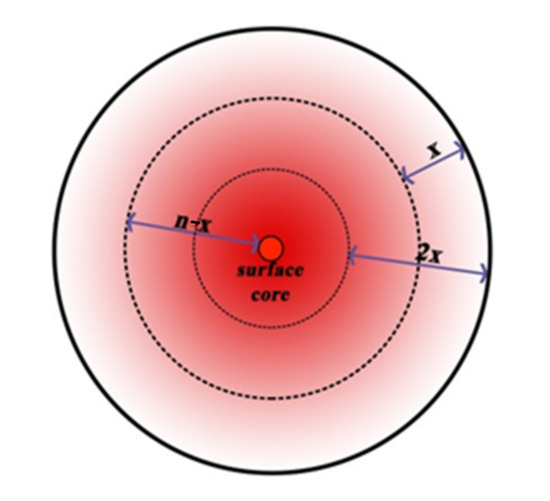
Figure 2.
Divided surfaces based on heat intensity.
Surface contiguity can be measured by measuring the proximity and density of pixels of hot surfaces. The closer this coefficient is to 11.1111 (for Landsat8 images), the more contiguous the hot surfaces are within the studied domain. Therefore, the contiguity of urban surfaces was quantified using the following equation:
where C represents the contiguity of an urban surface; represents the number of pixel centres in the image (pix/km2).
For Landsat images, C varies between 0 and 11.1111, although for other satellites, it may vary in different ranges depending on the pixel size of the images. The following equation can be used to calculate the area of hot surfaces based on the surface contiguity coefficient:
where Ca represents the contiguity surface area; Ps represents the pixel size.
Ca = C × Ps
To compare images from different satellites with different pixel sizes, one has to have a single coefficient. Since C varies from satellite to satellite depending on the pixel size, the contiguity can be calculated using the following formula:
where Cc represents the surface contiguity coefficient.
There are several methods used to check the correlation between two indicators with the help of software. The most common way to do so is to use the Pearson correlation coefficient:
where and Ȳ represent the means of variables x and y; Xi and Yi represent the variable values with i = 1, …, n.
The Pearson correlation coefficient varies between −1 and +1. The closer this coefficient is to zero, the lower the correlation, while the closer it is to −1 or 1, the higher the correlation. A correlation coefficient of +1 indicates a direct correlation and −1 indicates an inverse correlation [70].
2.4. Classification of Land Cover Types in Satellite Images
The impacts of different land covers on LST can be distinguished based on their differences in albedo [43,71] effect and evapotranspiration rate [49,72,73]. In this study, land cover types were classified using Sentinel satellite images because of their better resolution. The selected images were taken on 25 June 2018. Such classifications can be performed using supervised or unsupervised methods. In scientific research, it is common to use supervised methods equipped with learning algorithms. In such methods, the user provides a sample for each material and surface belonging to each class (e.g., forest cover), then the software detects the rest of the surfaces automatically based on the provided samples [74].
Previous studies have utilised various categories for the classification of land covers in satellite images depending on the scale of study area and dominant vegetation types [19,26,28,30,48,60,62]. These classifications often involve between 4 and 6 categories. In this paper, the maximum likelihood classification method was used due to the geographical scale and diversity of vegetation and ecosystems in Tehran. This method is one of the most commonly used methods for classification in remote sensing and provides a consistent approach to parameter estimation problems. Based on the maximum likelihood classification method, the land covers in Tehran were classified into six categories.
After classifying land covers in the satellite images, the accuracy and kappa coefficient values were calculated. The accuracy was measured by randomly selecting 100 points from each land cover category and checking whether the classifications matched the Google earth images. The higher the match between the classification map and these images, the closer the accuracy was to 100%. The Kappa coefficient was calculated using the following equation [75]:
where N represents the total number of pixels; m represents the number of classes; ∑Dijrepresents the total diagonal elements of an error matrix (the sum of correctly classified pixels in all images); Ri represents the total number of pixels in row i; Cj represents the total number of pixels in column j.
In this study, the accuracy and kappa coefficient were calculated as 88.17% and 0.91, respectively. Both the user’s accuracy and producer’s accuracy were checked for each of the six types of land cover, i.e., built-up areas, asphalt, forest, grassland, water, and barren surfaces. For these six types of land cover, the user’s accuracy rates were calculated as 89.71, 81.25, 91.24, 87.13, 91.18, and 89.42% and the producer’s accuracy rates were calculated as 83.49, 79.48, 88.39, 89.94, 92.11, and 90.56%, respectively.
3. Results
This section presents the results obtained by following the procedures described in the methodology section to identify the impacts of the form and size of different types of land covers on the intensity of UHIs.
3.1. Identification of Tehran’s UHIs Based on Land Cover Differences
This paper covers a case study from Tehran, Iran. Tehran is surrounded by mountains in the north, foothills in the centre, and desert in the south. Its altitude ranges from 900 to 1800 m above the mean sea level and increases from south to north [76]. It is located in a semi-arid climate zone [77].
To identify the microclimates of Tehran with an emphasis on detecting UHIs, first a land cover map of this city was created. As the land cover map in Figure 3 shows, Tehran’s area consists of 64.28% built-up lands, 3.07% urban forests, 4.65% green lands, 14.48% asphalt, 1.26% water, and12.24% barren soil. Then, the LST maps of the city for different times were created and the land covers that intensify the city’s UHIs were identified. Next, the relationships between these variables were investigated and the average temperature of each land cover type was calculated. The results, which are presented in Figure 4, show how much each land cover affects the intensity of UHIs.

Figure 3.
Tehran land cover (June 2018, Sentinel satellite). Retrieved from: https://scihub.copernicus.eu/dhus/#/home (accessed on 12 March 2020).
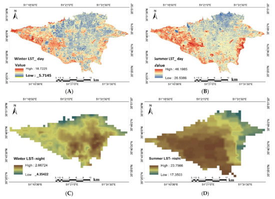
Figure 4.
Land surface temperature (LST) values from different weather conditions at day and night, during summer and winter: (A) winter day, 07:15, 5 February 2019, Landsat8; (B) summer day, 07:15, 28 July 2018, Landsat8; (C) 22:30, 5 February 2019, Modis; (D) 22:30, 28 July 2018, Modis. Retrieved from: (A,B) https://earthexplorer.usgs.gov/ (accessed on 12 March 2020); (C,D) https://search.earthdata.nasa.gov/search?ac=true (accessed on 12 March 2020).
Distribution of UHIs in Tehran
Urban surfaces generally absorb sunlight energy at short wavelengths and release it into the environment at long wavelengths, causing differences in ambient temperature [78]. As the maps in Figure 4 illustrate, the surface temperature ranges in Tehran in summer are 26.53–46.19 °C during the day and 17.35–23.17 °C at night, while in winter the ranges are −5.71–18.72 °C during the day and −4.35–2.66 °C at night. Therefore, the behaviour of urban heat islands in summer is almost similar to winter, although it increases in intensity so that the temperature increases sharply on the outskirts of the city.
The 22 municipal districts in Tehran have different dominant land cover types. The built-up areas are mostly concentrated in the central part of the city, including districts 10, 11, and 12, where on average 86.67% of the land is built-up. Forest cover is more concentrated in districts 1, 2, and 4 and in north, northwest, and eastern parts of the city. Grassland cover has no distinct concentration but can be found more in the northern and southern parts of the city. A large portion of asphalt cover in Tehran (32.06%) is in the city’s western part in district 21, which is known as Tehran’s industrial zone. The urban water bodies in Tehran do not have a specific concentration or pattern. About 30.01% of Tehran’s barren lands are concentrated in the eastern and western peripheries of the city, including districts 4, 9, 13, 14, 21, and 22. In general, Tehran’s microclimate in the northern part of this city is mostly affected by forests and urban green spaces, in the central part it is mostly affected by compact built-up areas, and in eastern and western parts and to some extent the southern part it is mostly affected by barren soil and asphalt covers.
Additionally, the temperature differences of land cover types vary from district to district, although they appear to follow certain patterns (Figure 5). The results of this diagram show that in all districts, barren soil (highlighted by yellow line) has the highest temperatures among land cover types for summer daytime samples, while the next highest temperatures are for asphalt cover, built-up areas, grasslands, forests, and water, in that order.

Figure 5.
Average temperatures by land cover type in different districts in Tehran for a sample summer day at 07:30 on 28 July 2018.
Figure 6 also shows the different effects of land cover types on urban heat island formation under different time conditions. Since Tehran has a hot and dry climate, the surfaces with the highest heat production rates during summer days are barren areas, followed by asphalt, built-up areas, grasslands, forests, and water, respectively, which produce lower temperatures than others. During summer nights, however, built-up areas have the highest temperatures, followed by asphalt, grasslands, barren lands, water, and forests. This paradoxical behaviour of barren cover areas is due to the cooling rate of soil, which is higher compared to other materials. When sunlight falls over arid and semi-arid regions predominantly containing soil cover, the soil quickly heats up, thereby making the barren parts warm. At night-time, however, the UHI is dominated by two factors: (1) the ability of materials to store solar radiation during the day; (2) the rate at which this energy is released at night. Barren cover, for example, which has heating effects during the day, shows cooling effects during the night. In winter, the thermal behaviours of different types of land cover are also different. During the daytime in winter, barren, asphalt, and grassland areas have highest surface temperatures, while at night-time in winter, the built-up areas give the highest surface temperatures.

Figure 6.
Land cover effects on surface temperature (LST) values and urban heat island formation under different weather conditions (summer and winter day- and night-time land cover spatial average LST values in Tehran).
The spatial growth and urban sprawl of Tehran over the last few decades are also pertinent factors. The peripheral areas of Tehran used to be dominated by farmland. However, the fast-paced growth of the city in the last few decades has led to considerable land use changes and the conversion of agricultural land covers to man-made land covers, as well as barren and soil cover types [29,79]. Such man-made and barren covers in the peripheral areas of Tehran are the main cause of the formation of UHIs during the daytime. Therefore, in order to reduce the effects of UHIs in Tehran, the development of greenbelts in the peripheral areas is of considerable importance.
3.2. Effects of Thermal Clusters’ Spatial Structures and Patterns on LST and UHI Values in Tehran
The formation and intensity of UHIs can be influenced not only by the type of land cover (which was discussed earlier) but also by other factors, including (a) the spatial structure, arrangement, or integration of thermal clusters and land covers (such as the placement of multiple smaller hot surfaces beside each other) and (b) the characteristics of land cover clusters, such as the dimensions, contiguity, and integration. Hence, a new land cover classification was made with the purpose of investigating the impacts of spatial patterns of land covers on UHIs. In this classification, land covers with relatively similar effects on UHIs temperature were put in the same groups, which here are called clusters. Three clusters were defined for this classification: hot (including asphalt and barren), cool (including water body and forest), and temperate (including built-up and grasslands).
Hot clusters represent the close placement or concentration of land covers that result in increased temperatures, such as asphalt and soil (Figure 7B), while cool clusters represent the close placement or concentration of land covers that keep temperatures low, such as water and green spaces (Figure 7A). In identifying cool and hot clusters, we utilised the kernel density estimation (KDE) method using GIS. Based on this method, we produced cluster-based density surfaces from point features, i.e., land cover data. Each cluster received a score according to its land covers, which then formed cool and hot clusters. Overall, 206.4 km2 of the area of this city is classified as hot surface areas (about 27% of the city is covered by barren soil and asphalt); about half of these hot surfaces have a high cluster contiguity, which results in more intensive heat generation.

Figure 7.
Main contiguity coefficients for cool and hot clusters in Tehran (pix/km2): hot clusters (A); cool clusters (B).
These clusters characterise different thermal behaviours:
- Thermal behaviour of hot clusters: During the daytime, upon exposure to direct sunlight, hot surfaces quickly absorb solar energy, which rapidly raises their temperature. Most notably, the soil heats up quickly and releases this heat into the environment; asphalt also heats up quickly because of its dark colour. After sunset, these surfaces release their stored heat almost as quickly as they gain heat during the day;
- Thermal behaviour of temperate clusters: Given their high heat capacity, temperate surfaces such as buildings and grass patches gradually absorb heat after sunrise and gradually release it into the environment after sunset. Thus, these clusters intensify UHIs at night-time and become the hottest clusters during these hours;
- Thermal behaviour of cool clusters: The evaporation mechanism prevents cool surfaces from absorbing heat, which makes them cooler than other surfaces, both at night and during the day.
It should be noted that dissimilar land covers behave differently in different climates. In a city such as Tehran, which has a relatively dry climate, the outer parts of the city experience a quick temperature drop after sunset, which results in the formation of a UHI in the central part of the city. This is because in hot and dry climates, barren soil is the hottest land cover and built-up areas have moderate temperatures. On the contrary, in temperate climates, built-up areas tend to be much hotter than the soil cover.
As shown in Figure 8, during the daytime Tehran’s peripheral areas (which are mostly shown on the right side of the graph, including districts 21, 22, 18, 19, 14, 15, and 9) have higher average temperatures than other areas, although during night-time, these areas rapidly lose heat and become cooler than the central parts of the city. During the daytime, the outer parts of the city are 2–3 °C warmer than the inner parts but at night-time the inner parts are 4–5 °C warmer than the outer parts.

Figure 8.
Average temperatures for hot and cool clusters in 22 districts (for a sample summer day on 28 July 2018 at 07:15).
In other words, as shown in Figure 9, there is a close relationship between the average surface temperature of each district and the presence of hot and cool surfaces (clusters) in that place. As the area of hot clusters in a district increases the UHI becomes more intense, then as the area of cool clusters increases the intensity of the UHI decreases.

Figure 9.
The relationship between the percentages of hot and cool clusters and the average temperatures in the districts of Tehran.
3.2.1. Identification of the Effects of Land and Thermal Cover Spatial Characteristics (Contiguity) and Cluster Dimensions on the Intensity of UHIs
Although the above-described analysis showed that the intensity of UHIs in a district generally depends on how much of it consists of hot and cool clusters, there were some exceptions to this rule, as some districts with small hot clusters (determined using Equation (7)) had high temperatures. On this basis, it was hypothesised that the intensity of UHIs is also a function of other factors such as the size and contiguity of clusters. This effect is represented by the surface contiguity coefficient (Equation (8)). The larger and more contiguous the hot cluster is, the greater the intensity of the associated UHI. This hypothesis was proven by the regression illustrated in Figure 10, which shows that the higher the average contiguity of hot clusters, the higher the average temperature and the greater the intensity of UHIs (R2 = 0.944) in a sample summer day.

Figure 10.
Hot cluster contiguity effects on land surface temperatures in Tehran for a sample summer day (28 July 2018 at 07:15). (R2 linear = 0.944; Pearson correlation = 0.972).
The cluster contiguity coefficient has a more pronounced effect in the peripheral parts of the city, which experiences increased intensity of UHIs. This is because of the presence of vast uninterrupted and undeveloped areas in these parts, which have a barren soil cover. As Figure 10 shows, the Cc does not have a dominant effect on hot and cool surfaces in the inner parts of the city because these parts have a mix of different land covers. However, for the peripheral parts of the city, including districts M2, M4, M5, M9, M13, M14, M15, M16, M18, M19, M21, and M22, which have vast continuous urban clusters, the Cc of hot clusters is more than 300. The Cc of cool clusters can also affect the intensity of UHIs. For districts M4, M5, M13, and M22, the Cc of cool clusters is more than 200, showing that these districts have good clustering.
3.2.2. Identification of the Effects of Cluster Colocation and Integration Patterns on the Intensity of UHIs
Another cause of behavioural differences between thermal clusters is the pattern of colocation of land cover clusters, which in this study is represented by the cluster mixing coefficient (cluster mixing is defined based on the percentage of the sides of a cluster that border another cluster). As shown in Table 1, the presence of hot and cool clusters in one area in the vicinity of each other affects the intensity of UHIs (Figure 11). In districts M4, M13, and M22, the copresence and partial mixing of two hot and cool clusters (see Table 1) has decreased the average LST of hot clusters by approximately 1.5–2.5 °C. On the contrary, in district M5, because of the separation of hot and cool clusters, the Cc has decreased the cooling effect of the cool cluster by 1 °C.

Table 1.
The average temperature, density, and mixing coefficient values for hot and cool clusters in Tehran on a sample summer day.
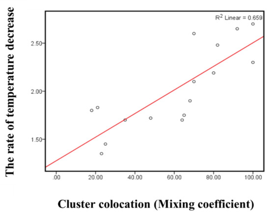
Figure 11.
Cluster mixing effect on temperature reduction (R2 linear = 0.659).
The higher the Cc of the hot clusters, the higher the intensity of the UHIs. The presence of cool clusters is highly effective in preventing the formation of UHIs from hot clusters. For example, while districts 4 and 5 have the same percentage of hot clusters, the hot clusters in district 4 are more fragmented by cool clusters, which has resulted in a lower LST in this district than in district M21. Additionally, although districts M9, M18, and M19 have lower percentages of hot clusters than M22, they have higher LSTs, as their hot clusters are less mixed with cool clusters.
3.3. Investigation of the Effects of Form Characteristics of Land Covers on the Formation of UHIs
The previous sections explained firstly how the colocation or placement of hot surfaces next to each other results in the creation of larger contiguous hot clusters, leading to increased contiguity coefficient and ultimately intensified UHI, and secondly how the mixing of hot and cool clusters reduces the UHI effect. This section discusses the effects of form characteristics of land cover clusters, including their dimensions and size, on the formation and intensification of UHIs. For this discussion, the main hot and cool clusters of Tehran were analysed in order to determine the minimum cluster size and dimensions that prevent the intensification of UHI; that is, this section presents a quantitative investigation of why the cluster contiguity affects the intensification of UHIs. For this purpose, it is first necessary to define the concept of optimal distance.
Determination of Optimal Contiguity Distance for Thermal Clusters
To determine the optimal distance of land covers in Tehran, covers were grouped into a few clusters with similar thermal conditions. This approach was chosen as the greater size and contiguity of the resulting clusters compared to individual covers makes it easier to analyse their effects on UHIs. The main hot and cool clusters of Tehran were identified by grouping the points whose Cc values fell in the last category into these clusters. Therefore, the main hot clusters were areas with Cc > 700 and the main cool clusters were areas with Cc > 350. As shown in Figure 8, nine main hot clusters (B) and three main cool clusters (A) were found to be affecting the micro-climates of Tehran.
To investigate the effects of cluster size and contiguity on the formation of UHIs in Tehran, the Pearson correlation formula was used to identify correlations between temperature and distance from the centres of clusters (Figure 12). The correlation coefficients obtained for the main hot clusters of Tehran, which are mostly located in the peripheral parts of this city, were as follows: Doshan hill (−0.636), Westlands (−0.441), Ghalemorghi (−565), Gomrok (−0.648), Larak (−0.5), Mehrabad airport (−0.562), Army lands (−0.717), Northern Sayad (−0.509), and Pardisan park (−0.741).
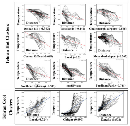
Figure 12.
The effects of cluster size and contiguity on the formation of UHIs in Tehran (showing the Pearson correlations between Tehran’s main hot and cool clusters temperatures and distances from the centres of clusters).
In the three main cool clusters of Tehran, which are mostly located in the northern part of this city, temperature increases as we move away from the centre and toward the edges (Figure 13). This is the opposite of what occurs in hot clusters. For the three main cool clusters, which are Larak, Darake, and Dehkade Olampic, the Pearson correlation coefficient values for the relationship between temperature and distance from the edges were calculated as 0.724, 0.578, and 0.690, respectively.

Figure 13.
Temperature profile of land cover types in Tehran.
The present study shows that the contiguity of land cover surfaces has an intensifying effect on UHIs, and this effect becomes particularly dominant when the surface is vast and continuous. The thermal effect of a cover, whether hot or cool, intensifies as we move away from the edges and get closer to the centre of the surface. Hence, interrupting the continuity of large land cover surfaces can reduce their thermal effect. However, hot and cool covers respond differently to such interruptions. For cool covers such as wooded areas and forests, the thermal effect is decreasing, meaning that temperature decreases as we move away from the edge and closer to the centre, while the rate of temperature change is contingent upon the distance between the edge and the centre. Therefore, for these clusters, the greater the distance from the edge to the centre, the lower the temperature. However, for hot clusters, the temperature increases as you move away from the edges and closer to the centre. Thus, for both hot and cool clusters, the thermal effect intensifies towards the centre. Under this assumption, for the clusters shown in Figure 12, the thermal behaviour is constant up to the distance x but intensifies thereafter (i.e., at the radius n − x). Therefore, after identifying this optimal distance for each type of cover, it will be possible to break the continuity of hot covers through measures such as planting trees or building water corridors at these distances. This could be an especially effective measure for hot and dry areas, where water scarcity makes it difficult and expensive to build and maintain large green spaces.
The optimal distance x has an extensive impact on UHIs. As shown in Figure 13, the spatial structures of the six land covers considered in this study have different optimal distances from the edge, which are distinguished by natural breaks in the data charts. Because of the heterogeneity of materials used in buildings, the optimal distance for “built-up areas” varies from place to place and does not follow any specific pattern. This means that this distance can only be estimated by accurate analysis and modelling of buildings in a specific domain. For other covers, however, this distance can be accurately estimated. The optimal distance is 150 m for forest cover, 550 m for grasslands, 100 m for asphalt, 200 m for water bodies, and 220 m for barren soil. To reduce UHIs, it is more important to estimate this distance for hot clusters than for cool clusters. This is because in cool clusters the temperature decreases from 1.5 to 2.5 °C at the optimal distance and decreases at a much lower rate over longer distances (n − x). However, in hot clusters, the temperature increases by about 0.5 °C at the optimal distance and very rapidly over long distances, so much so that it rises by 2.5–4 °C at a distance of 2x.
4. Discussion
The type and distribution of land covers play key roles in the formation of UHIs due to their direct impact on LSTs and changes in urban microclimates. The effects of land covers on UHIs has been extensively investigated in the UHI literature. However, since different land covers can have different impacts on UHIs depending on the local climate, this study investigated the effects of land covers in the semi-arid climate of the Tehran metropolitan area, which is an under-researched climate in this regard. We used the concept of contiguity to analyse how the thermal behaviour and effects of different clusters change depending on the pattern of spatial development. Analysing the thermal behaviour of land covers in the Tehran metropolitan area yielded the following results. First, the contributions of the six categories of land covers to the LSTs in summer were as follows: soil > asphalt > built-up areas > grassland > forest > water; therefore, soil cover in semi-arid climates has the highest contribution to the LST. Although it is worth mentioning that the thermal behaviours identified for these cover types are true for semi-arid climates in summer but not necessarily for other seasons or other climates. The highest temperature in the studied area was related to barren soil and asphalt cover types, while the lowest was related to water bodies and forest.
Second, almost 17% of the total land cover in Tehran is barren soil and only 4% of the land is covered with forests and urban green spaces. Tehran is located in a hot and dry region with severe water scarcity, which makes the existing solutions and strategies presented in the international literature ineffective in dealing with UHI and undesirable microclimates. Strategies that rely on developing large-scale green spaces or water bodies only work in countries with high water resources that can develop and maintain green spaces. Therefore, this study attempted to find sustainable and ecological solutions that are specific and relevant for cities in semi-arid climates. Analysis of the optimal sizes of land covers and their combined effects on each other showed that mixing land uses to interrupt the continuity effects of large cool and hot surfaces (breaking them into smaller surfaces) and also combining them with each other is the most suitable and sustainable solution for reducing UHIs in the studied hot and dry climate of Tehran.
Third, in this study, a coefficient called surface contiguity was used to determine the optimal size of land covers and clusters. This is in line with previous studies that utilised this concept in the analysis of continuity of specific sites. The authors measured the effect of contiguity in land cover on the formation of UHIs. The results showed that increasing the contiguity of hot land covers (e.g., barren soil and asphalt) intensifies the growth of UHIs, while on the contrary increasing the contiguity of cool land covers reduces their cooling effect. Determining the optimal size of each specific land cover type helps Tehran’s city planners and decision-makers to determine what land uses to mix and where to place certain activities and zones in order to maximise the impact on the city’s microclimate. This study found that contiguity seems to have a great impact on UHIs both at micro and macro levels. To investigate this impact, land covers were divided into three clusters: hot, cool, and temperate. The more compact the hot and cool clusters are, the more contiguous they become, which leads to an increase in UHIs. The results of this study suggest that for every 100 pix/km2 increase, the cluster temperature increases by approximately 0.7–1 °C. Additionally, placing cool clusters near or in combination with hot clusters interrupts the effects of hot clusters, leading to significant temperature reductions. The temperature differences between the peripheral parts of the Tehran metropolitan area, where hot clusters are more contiguous, and the central part of this city, where land covers are more mixed, reach as much as 4–5 °C. These results suggest that urban areas with more mixed land uses tend to experience less intense UHIs, and vice versa.
Land cover types and sizes, contiguity, and distribution are among the most important determinants of the formation and intensity of UHIs. Because of the environmental-climatic limitations of Tehran, the common solutions recommended in the UHI literature, which mostly involve building more green spaces, cannot be applied to this city on a large scale. To determine the optimal distance for breaking (interrupting) the continuity of hot surfaces in this city, 9 hot clusters and 3 cool clusters in the area were identified and carefully investigated using appropriate metrics. The results of this investigation showed that in hot clusters, temperature decreases as we move away from the centre of the cluster and toward its edges, but in cool clusters, the same movement decreases the intensity of the cooling effect. Therefore, one can determine for each cluster the optimal distance at which the intervention has maximal effect. For example, the temperature increased by about 0.5 °C at the optimal distance x from the edge of a hot cluster, but it increased by 2.5–4 °C at the distance of 2x. Therefore, the temperature of the centre of a hot cluster depends on its distance from the edge of the cluster. Next, the optimal dimensions of each land cover for making optimal sustainable use of urban lands to deal with the UHI problem were determined. The optimal distances were calculated as 250 m (from the edge) for barren soil and 150 m (from the edge) for forests. These figures help urban planners and decision-makers to prepare more effective plans and strategies for reducing UHIs through the mixing of different land covers. Overall, planning interventions such as developing linear parks instead of large-scale continuous green spaces, mixing hot and cool land uses to interrupt the thermal effects of hot land covers, and ensuring a proportionate distribution of small parks in affected neighbourhoods are expected to be effective in reducing UHIs.
5. Conclusions
This research assessed the effects of thermal-spatial behaviours of land covers on UHIs in the semi-arid climate of Tehran and made three main contributions to the UHI literature. First, acknowledging that different land covers can have different impacts on UHIs, depending on the local climate, this study investigated the effects of land covers in the semi-arid climate of the Tehran metropolitan area, which is an under-researched climate in this regard. The majority of UHI studies are conducted in the cold-and-humid climates of Europe and North America and the solutions and strategies presented in these studies are not applicable to cities such as Tehran, which has different condition in terms of climate and land cover. Generalising the findings of European and North American studies and applying them to cities located in a semi-arid climate cannot solve the problem of UHIs in these cities. This is particularly important as time and financial resources are limited and adapting incorrect strategies can lead to wasted resources without achieving considerable positive outcomes. Second, unlike existing studies on the UHIs in semi-arid climates, such as the study by Mathew et al. [80] that compared urban and rural areas, we conducted our investigation at the inner-city scale, which required higher resolution images such as those offered by Landsat8. However, Landsat8 only offers images of Tehran at a specific day time and does not provide any images of Tehran at night. To compensate for this, we used data from MODIS, which offers a wider range of images throughout day and night. Although MODIS images are of lower resolution compared to Landsat8, they provide images of Tehran at night. Therefore, we combined data from MODIS and Landsat8 to cover a wider range of times and places whilst increasing the accuracy. Third, in addition to assessing the effects of land covers on the formation of UHIs, we took account of the influences of different spatial patterns of thermal clusters on UHIs in our analysis. Consideration of the spatial patterns of thermal clusters enabled us to provide planners and decision makers with practical recommendations that are specific and relevant to the context of cities located in a semi-arid climate. We highlighted the importance of considerations concerning the type and location of land uses and land surfaces in reducing the effects of UHIs when developing large-scale green spaces is not feasible due to water shortages. Further research is required to investigate the diurnal surface temperature variations of different land covers at different times of day and night throughout the year and their effects on UHIs in cities located in semi-arid climates. Additionally, consideration of the differences between central cities and their peripheral areas in terms of UHIs at the regional scale would be a fruitful area for further work.
Author Contributions
Conceptualisation, S.N.-T. and M.A.; methodology, S.N.-T. and M.A.; software, M.A.; writing—original draft preparation, S.N.-T., M.A., S.S. and E.S.; writing—review and editing, S.N.-T., M.A., S.S. and E.S.; visualisation, M.A.; supervision, S.N.-T.; funding acquisition, S.S. All authors have read and agreed to the published version of the manuscript.
Funding
This research received no external funding.
Institutional Review Board Statement
Not applicable.
Informed Consent Statement
Not applicable.
Data Availability Statement
Data sharing is not applicable to this article.
Conflicts of Interest
The authors declare no conflict of interest.
References
- Chen, X.L.; Zhao, H.M.; Li, P.X.; Yin, Z.Y. Remote sensing image-based analysis of the relationship between urban heat island and land use/cover changes. Remote Sens. Environ. 2006, 104, 133–146. [Google Scholar] [CrossRef]
- Sen, S.; Roesler, J. Thermal and optical characterization of asphalt field cores for microscale urban heat island analysis. Constr. Build. Mater. 2019, 217, 600–611. [Google Scholar] [CrossRef]
- Zhang, Y.; Sun, L. Spatial-temporal impacts of urban land use land cover on land surface temperature: Case studies of two Canadian urban areas. Int. J. Appl. Earth Obs. Geoinf. 2019, 75, 171–181. [Google Scholar] [CrossRef]
- Zhao, W.; Li, A.; Huang, Q.; Gao, Y.; Li, F.; Zhang, L. An improved method for assessing vegetation cooling service in regulating thermal environment: A case study in Xiamen, China. Ecol. Indic. 2019, 98, 531–542. [Google Scholar] [CrossRef]
- Wang, C.; Wang, Z.H.; Wang, C.; Myint, S.W. Environmental cooling provided by urban trees under extreme heat and cold waves in U.S. cities. Remote Sens. Environ. 2019, 227, 28–43. [Google Scholar] [CrossRef]
- Wang, Y.; Zhan, Q.; Ouyang, W. How to quantify the relationship between spatial distribution of urban waterbodies and land surface temperature? Sci. Total. Environ. 2019, 671, 1–9. [Google Scholar] [CrossRef]
- Ward, K.; Lauf, S.; Kleinschmit, B.; Endlicher, W. Heat waves and urban heat islands in Europe: A review of relevant drivers. Sci. Total. Environ. 2016, 569–570, 527–539. [Google Scholar] [CrossRef]
- Onishi, A.; Cao, X.; Ito, T.; Shi, F.; Imura, H. Evaluating the potential for urban heat-island mitigation by greening parking lots. Urban For. Urban Green. 2010, 9, 323–332. [Google Scholar] [CrossRef]
- Madanian, M.; Soffianian, A.R.; Koupai, S.S.; Pourmanafi, S.; Momeni, M. The study of thermal pattern changes using Landsat-derived land surface temperature in the central part of Isfahan province. Sustain. Cities Soc. 2018, 39, 650–661. [Google Scholar] [CrossRef]
- Doan, V.Q.; Kusaka, H.; Nguyen, T.M. Roles of past, present, and future land use and anthropogenic heat release changes on urban heat island effects in Hanoi, Vietnam: Numerical experiments with a regional climate model. Sustain. Cities Soc. 2019, 47, 101479. [Google Scholar] [CrossRef]
- Li, X.; Zhou, Y.; Yu, S.; Jia, G.; Li, H.; Li, W. Urban heat island impacts on building energy consumption: A review of approaches and findings. Energy 2019, 174, 407–419. [Google Scholar] [CrossRef]
- Li, H.; Meier, F.; Lee, X.; Chakraborty, T.; Liu, J.; Schaap, M.; Sodoudi, S. Interaction between urban heat island and urban pollution island during summer in Berlin. Sci. Total. Environ. 2018, 636, 818–828. [Google Scholar] [CrossRef]
- Lowe, S.A. An energy and mortality impact assessment of the urban heat island in the US. Environ. Impact Assess. Rev. 2016, 56, 139–144. [Google Scholar] [CrossRef]
- Huang, Q.; Huang, J.; Yang, X.; Fang, C.; Liang, Y. Quantifying the seasonal contribution of coupling urban land use types on Urban Heat Island using Land Contribution Index: A case study in Wuhan, China. Sustain. Cities Soc. 2019, 44, 666–675. [Google Scholar] [CrossRef]
- Elliot, T.; Babí Almenar, J.; Rugani, B. Modelling the relationships between urban land cover change and local climate regulation to estimate urban heat island effect. Urban For. Urban Green. 2020, 50, 126650. [Google Scholar] [CrossRef]
- Nastran, M.; Kobal, M.; Eler, K. Urban heat islands in relation to green land use in European cities. Urban For. Urban Green. 2019, 37, 33–41. [Google Scholar] [CrossRef] [Green Version]
- Rotem-Mindali, O.; Michael, Y.; Helman, D.; Lensky, I.M. The role of local land-use on the urban heat island effect of Tel Aviv as assessed from satellite remote sensing. Appl. Geogr. 2015, 56, 145–153. [Google Scholar] [CrossRef]
- Steeneveld, G.J.; Koopmans, S.; Heusinkveld, B.G.; Theeuwes, N.E. Refreshing the role of open water surfaces on mitigating the maximum urban heat island effect. Landsc. Urban Plan. 2014, 121, 92–96. [Google Scholar] [CrossRef]
- Wang, Y.C.; Hu, B.K.; Myint, S.W.; Feng, C.C.; Chow, W.T.; Passy, P.F. Patterns of land change and their potential impacts on land surface temperature change in Yangon, Myanmar. Sci. Total. Environ. 2018, 643, 738–750. [Google Scholar] [CrossRef]
- Taleb, D.; Abu-Hijleh, B. Urban heat islands: Potential effect of organic and structured urban configurations on temperature variations in Dubai, UAE. Renew. Energy 2013, 50, 747–762. [Google Scholar] [CrossRef]
- Liang, Z.; Wu, S.; Wang, Y.; Wei, F.; Huang, J.; Shen, J.; Li, S. The relationship between urban form and heat island intensity along the urban development gradients. Sci. Total. Environ. 2020, 708, 135011. [Google Scholar] [CrossRef]
- Alobaydi, D.; Bakarman, M.A.; Obeidat, B. The impact of urban form configuration on the urban heat island: The case study of Baghdad, Iraq. Procedia Eng. 2016, 145, 820–827. [Google Scholar] [CrossRef]
- Long, L.C.; D’Amico, V.; Frank, S.D. Urban forest fragments buffer trees from warming and pests. Sci. Total. Environ. 2019, 658, 1523–1530. [Google Scholar] [CrossRef] [PubMed]
- Gao, F.; Hilker, T.; Zhu, X.; Anderson, M.; Masek, J.; Wang, P.; Yang, Y. Fusing landsat and MODIS data for vegetation monitoring. IEEE Geosci. Remote Sens. Mag. 2015, 3, 47–60. [Google Scholar] [CrossRef]
- Greene, C.S.; Kedron, P.J. Beyond fractional coverage: A multilevel approach to analyzing the impact of urban tree canopy structure on surface urban heat islands. Appl. Geogr. 2018, 95, 45–53. [Google Scholar] [CrossRef]
- Grigora, G.; Uri, B. Land use/land cover changes dynamics and their effects on surface urban heat island in Bucharest, Romania. Int. J. Appl. Earth Obs. Geoinf. 2019, 80, 115–126. [Google Scholar] [CrossRef]
- Delgado, J.D.; Arroyo, N.L.; Arévalo, J.R.; Fernández-ernández-Palacios, J.M. Edge effects of roads on temperature, light, canopy cover, and canopy height in l pine forests (Tenerife, Canary Islands). Landsc. Urban Plan. 2007, 81, 328–340. [Google Scholar] [CrossRef]
- Ali, J.M.; Marsh, S.H.; Smith, M.J. A comparison between London and Baghdad surface urban heat islands and possible engineering mitigation solutions. Sustain. Cities Soc. 2017, 29, 159–168. [Google Scholar] [CrossRef] [Green Version]
- Bokaie, M.; Zarkesh, M.K.; Arasteh, P.D.; Hosseini, A. Assessment of urban heat island based on the relationship between land surface temperature and land use/land cover in Tehran. Sustain. Cities Soc. 2016, 23, 94–104. [Google Scholar] [CrossRef]
- Mathew, A.; Khandelwal, S.; Kaul, N.; Chauhan, S. Analyzing the diurnal variations of land surface temperatures for surface urban heat island studies: Is time of observation of remote sensing data important? Sustain. Cities Soc. 2018, 40, 194–213. [Google Scholar] [CrossRef] [Green Version]
- Jiang, L.; Wang, S. Enhancing heat release of asphalt pavement by a gradient heat conduction channel. Constr. Build. Mater. 2020, 230, 117018. [Google Scholar] [CrossRef]
- Akbari, H.; Kolokotsa, D. Three decades of urban heat islands and mitigation technologies research. Energy Build. 2016, 133, 834–842. [Google Scholar] [CrossRef]
- Farhadi, H.; Faizi, M.; Sanaieian, H. Mitigating the urban heat island in a residential area in Tehran: Investigating the role of vegetation, materials, and orientation of buildings. Sustain. Cities Soc. 2019, 46, 101448. [Google Scholar] [CrossRef]
- Oke, T.R. City size and the urban heat island. Atmos. Environ. (1967) 1973, 7, 769–779. [Google Scholar] [CrossRef]
- Khamchiangta, D.; Dhakal, S. Physical and non-physical factors driving urban heat island: Case of Bangkok metropolitan administration, Thailand. J. Environ. Manag. 2019, 248, 109285. [Google Scholar] [CrossRef]
- Shojaei, P.; Gheysari, M.; Myers, B.; Eslamian, S.; Shafieiyoun, E.; Esmaeili, H. Effect of different land cover/use types on canopy layer air temperature in an urban area with a dry climate. Build. Environ. 2017, 125, 451–463. [Google Scholar] [CrossRef]
- Yue, W.; Liu, X.; Zhou, Y.; Liu, Y. Impacts of urban configuration on urban heat island: An empirical study in China mega-cities. Sci. Total. Environ. 2019, 671, 1036–1046. [Google Scholar] [CrossRef]
- Debbage, N.; Shepherd, J.M. The urban heat island effect and city contiguity. Comput. Environ. Urban Syst. 2015, 54, 181–194. [Google Scholar] [CrossRef]
- Yadav, N.; Sharma, C. Spatial variations of intra-city urban heat island in megacity Delhi. Sustain. Cities Soc. 2018, 37, 298–306. [Google Scholar] [CrossRef]
- Li, Y.; Zhang, H.; Kainz, W. Monitoring patterns of urban heat islands of the fast-growing Shanghai metropolis, China: Using time-series of Landsat TM/ETM+ data. Int. J. Appl. Earth Obs. Geoinf. 2012, 19, 127–138. [Google Scholar] [CrossRef]
- De Faria Peres, L.; de Lucena, A.J.; Rotunno Filho, O.C.; de Almeida França, J.R. The urban heat island in Rio de Janeiro, Brazil, in the last 30 years using remote sensing data. Int. J. Appl. Earth Obs. Geoinf. 2018, 64, 104–116. [Google Scholar] [CrossRef]
- Silva, J.S.; Silva, R.M.; da Santos, C.A.G. Spatiotemporal impact of land use/land cover changes on urban heat islands: A case study of Paço do Lumiar, Brazil. Build. Environ. 2018, 136, 279–292. [Google Scholar] [CrossRef]
- Wallner, S.; Kocifaj, M. Impacts of surface albedo variations on the night sky brightness—A numerical and experimental analysis. J. Quant. Spectrosc. Radiat. Transf. 2019, 239, 106648. [Google Scholar] [CrossRef]
- Voogt, J.A.; Oke, T.R. Thermal remote sensing of urban climates. Remote Sens. Environ. 2003, 86, 370–384. [Google Scholar] [CrossRef]
- Wang, Y.; Berardi, U.; Akbari, H. Comparing the effects of urban heat island mitigation strategies for Toronto, Canada. Energy Build. 2016, 114, 2–19. [Google Scholar] [CrossRef]
- Li, H.; Zhou, Y.; Wang, X.; Zhou, X.; Zhang, H.; Sodoudi, S. Quantifying urban heat island intensity and its physical mechanism using WRF/UCM. Sci. Total. Environ. 2019, 650, 3110–3119. [Google Scholar] [CrossRef] [PubMed]
- Zhou, X.; Chen, H. Impact of urbanization-related land use land cover changes and urban morphology changes on the urban heat island phenomenon. Sci. Total. Environ. 2018, 635, 1467–1476. [Google Scholar] [CrossRef] [PubMed]
- Dai, Z.; Guldmann, J.M.; Hu, Y. Spatial regression models of park and land-use impacts on the urban heat island in central Beijing. Sci. Total. Environ. 2018, 626, 1136–1147. [Google Scholar] [CrossRef]
- Li, W.; Bai, Y.; Chen, Q.; He, K.; Ji, X.; Han, C. Discrepant impacts of land use and land cover on urban heat islands: A case study of Shanghai, China. Ecol. Indic. 2014, 47, 171–178. [Google Scholar] [CrossRef]
- Sheng, L.; Tang, X.; You, H.; Gu, Q.; Hu, H. Comparison of the urban heat island intensity quantified by using air temperature and Landsat land surface temperature in Hangzhou, China. Ecol. Indic. 2017, 72, 738–746. [Google Scholar] [CrossRef]
- Gao, M.; Chen, S.; Chen, W.; Wang, W.; Liang, H.; Hao, G.; Liu, K. Spatiotemporal variation of heat fl uxes in Beijing with land use change from 1997 to 2017. Phys. Chem. Earth Parts A/B/C 2019, 110, 51–60. [Google Scholar] [CrossRef]
- Firozjaei, M.K.; Kiavarz, M.; Alavipanah, S.K.; Lakes, T.; Qureshi, S. Monitoring and forecasting heat island intensity through multi-temporal image analysis and cellular automata-Markov chain modelling: A case of Babol city, Iran. Ecol. Indic. 2018, 91, 155–170. [Google Scholar] [CrossRef]
- Haashemi, S.; Weng, Q.; Darvishi, A.; Alavipanah, S.K. Seasonal variations of the surface urban heat island in a Semi-Arid city. Remote Sens. 2016, 8, 352. [Google Scholar] [CrossRef] [Green Version]
- Azevedo, J.A.; Chapman, L.; Muller, C.L. Quantifying the daytime and night-time urban heat island in Birmingham, UK: A comparison of satellite derived land surface temperature and high resolution air temperature observations. Remote Sens. 2016, 8, 153. [Google Scholar] [CrossRef] [Green Version]
- Tomlinson, C.; Chapman, L.; Thornes, J.; Baker, C. Including the urban heat island in spatial heat health risk assessment strategies: A case study for Birmingham, UK. Int. J. Health Geogr. 2011, 10, 1–4. [Google Scholar] [CrossRef] [Green Version]
- Yin, C.; Yuan, M.; Lu, Y.; Huang, Y.; Liu, Y. Effects of urban form on the urban heat island effect based on spatial regression model. Sci. Total. Environ. 2018, 634, 696–704. [Google Scholar] [CrossRef]
- Cai, Z.; Han, G.; Chen, M. Do water bodies play an important role in the relationship between urban form and land surface temperature? Sustain. Cities Soc. 2018, 39, 487–498. [Google Scholar] [CrossRef]
- Lee, H.S.; Trihamdani, A.R.; Kubota, T.; Iizuka, S.; Phuong, T.T.T. Impacts of land use changes from the Hanoi Master Plan 2030 on urban heat islands: Part 2. Sustain. Cities Soc. 2017, 31, 95–108. [Google Scholar] [CrossRef]
- Boyte, S.P.; Wylie, B.K.; Major, D.J. Cheatgrass percent cover change: Comparing recent estimates to climate change-driven predictions in the northern Great Basin. Rangel. Ecol. Manag. 2016, 69, 265–279. [Google Scholar] [CrossRef]
- Tran, D.X.; Pla, F.; Latorre-Carmona, P.; Myint, S.W.; Caetano, M.; Kieu, H.V. Characterizing the relationship between land use land cover change and land surface temperature. ISPRS J. Photogramm. Remote Sens. 2017, 124, 119–132. [Google Scholar] [CrossRef] [Green Version]
- Li, T.; Meng, Q. A mixture emissivity analysis method for urban land surface temperature retrieval from Landsat 8 data. Landsc. Urban Plan. 2018, 179, 63–71. [Google Scholar] [CrossRef]
- Fathizad, H.; Tazeh, M.; Kalantari, S.; Shojaei, S. The investigation of spatiotemporal variations of land surface temperature based on land use changes using NDVI in southwest of Iran. J. Afr. Earth Sci. 2017, 134, 249–256. [Google Scholar] [CrossRef]
- Aguilar-Lome, J.; Espinoza-Villar, R.; Espinoza, J.C.; Rojas-Acuña, J.; Willems, B.L.; Leyva-Molina, W.M. Elevation-dependent warming of land surface temperatures in the Andes assessed using MODIS LST time series (2000–2017). Int. J. Appl. Earth Obs. Geoinf. 2019, 77, 119–128. [Google Scholar] [CrossRef]
- Haynes, M.W.; Horowitz, F.G.; Sambridge, M.; Gerner, E.J.; Beardsmore, G.R. Australian mean land-surface temperature. Geothermics 2018, 72, 156–162. [Google Scholar] [CrossRef]
- Duan, S.B.; Li, Z.L.; Li, H.; Göttsche, F.M.; Wu, H.; Zhao, W.; Leng, P.; Zhang, X.; Coll, C. Remote Sensing of Environment Validation of Collection 6 MODIS land surface temperature product using in situ measurements. Remote Sens. Environ. 2019, 225, 16–29. [Google Scholar] [CrossRef] [Green Version]
- Ayanlade, A.; Howard, M.T. Land surface temperature and heat fluxes over three cities in Niger Delta. J. Afr. Earth Sci. 2018, 151, 54–66. [Google Scholar] [CrossRef]
- Mahato, S.; Pal, S. Influence of land surface parameters on the spatio-patio-seasonal land surface temperature regime in West Bengal, India. Adv. Space Res. 2018, 63, 172–189. [Google Scholar] [CrossRef]
- Manickathan, L.; Defraeye, T.; Allegrini, J.; Derome, D.; Carmeliet, J. Parametric study of the influence of environmental factors and tree properties on the transpirative cooling effect of trees. Agric. For. Meteorol. 2018, 248, 259–274. [Google Scholar] [CrossRef] [Green Version]
- Ahmadpoor, N.; Shahab, S. Realising the value of green space: A planners’ perspective on the COVID-19 pandemic. Town Plan. Rev. 2021, 92, 49–55. [Google Scholar] [CrossRef]
- Adler, J.; Parmryd, I. Quantifying colocalization by correlation: The pearson correlation coefficient is superior to the Mander’s overlap coefficient. Cytom. Part A 2010, 77, 733–742. [Google Scholar] [CrossRef] [PubMed]
- R Rinehart, A.J.; Vivoni, E.R.; Brooks, P.D. Effects of vegetation, albedo, and solar radiation sheltering on the distribution of snow in the Valles Caldera, New Mexico. Ecohydrol. Ecosyst. Land Water Process. Interact. Ecohydrogeomorphol. 2008, 1, 253–270. [Google Scholar] [CrossRef]
- Hu, Y.; Hou, M.; Zhao, C.; Zhen, X.; Yao, L.; Xu, Y. Human-induced changes of surface albedo in Northern China from 1992–2012. Int. J. Appl. Earth Obs. Geoinf. 2019, 79, 184–191. [Google Scholar] [CrossRef]
- Ow, L.F.; Ghosh, S.; Yusof, M.L.M. Growth of Samanea Saman: Estimated cooling potential of this tree in an urban environment. Urban For. Urban Green. 2019, 41, 264–271. [Google Scholar] [CrossRef]
- Arsiso, B.K.; Tsidu, G.M.; Stoffberg, G.H.; Tadesse, T. Influence of urbanization-driven land use/cover change on climate: The case of Addis Ababa, Ethiopia. Phys. Chem. Earth Parts A/B/C 2018, 105, 212–223. [Google Scholar] [CrossRef]
- Bogoliubova, A.; Tymków, P. Accuracy assessment of automatic image processing for land cover classification of St. Petersburg protected area. Acta Sci. Pol. Geod. Descr. Terrarum 2014, 13, 5–22. [Google Scholar]
- Moghadas, M.; Asadzadeh, A.; Vafeidis, A.; Fekete, A.; Kötter, T. A multi-criteria approach for assessing urban flood resilience in Tehran, Iran. Int. J. Disaster Risk Reduct. 2019, 35, 101069. [Google Scholar] [CrossRef]
- Tayyebi, A.; Sha, H.; Tayyebi, A.H. Analyzing long-term spatio-patio-temporal patterns of land surface temperature in response to rapid urbanization in the mega-city of Tehran. Land Use Policy 2017, 71, 459–469. [Google Scholar] [CrossRef]
- Oke, T.R.; Mills, G.; Christen, A.; Voogt, J.A. Urban Climates; Cambridge University Press: Cambridge, UK, 2017. [Google Scholar] [CrossRef] [Green Version]
- Gao, Y.; Shahab, S.; Ahmadpoor, N. Morphology of urban villages in China: A case study of dayuan village in Guangzhou. Urban Sci. 2020, 4, 23. [Google Scholar] [CrossRef]
- Mathew, A.; Khandelwal, S.; Kaul, N. Analysis of diurnal surface temperature variations for the assessment of surface urban heat island effect over Indian cities. Energy Build. 2018, 159, 271–295. [Google Scholar] [CrossRef]
Publisher’s Note: MDPI stays neutral with regard to jurisdictional claims in published maps and institutional affiliations. |
© 2021 by the authors. Licensee MDPI, Basel, Switzerland. This article is an open access article distributed under the terms and conditions of the Creative Commons Attribution (CC BY) license (https://creativecommons.org/licenses/by/4.0/).