Abstract
The accurate measurement of the PM individual exposure level is a key issue in the study of health effects. However, the lack of historical data and the minute coverage of ground monitoring points are obstacles to the study of such issues. Based on the aerosol optical depth provided by NASA, combined with ground monitoring data and meteorological data, it is an effective method to estimate the near-ground concentration of PM. With the deepening of related research, the models used have developed from univariate and multivariate linear models to nonlinear models such as support vector machine, random forest model, and deep learning neural network model. Among them, the depth neural network model has better performance. However, in the existing research, the variables used are input into the same neural network together, that is, the complex relationship caused by the lag effect of features and the correlation and partial correlation between features have not been considered. The above neural network framework can not be well applied to the complex situation of atmospheric systems and the estimation accuracy of the model needs to be improved. This is the first problem that we need to be overcome. Secondly, in the missing data value processing, the existing studies mostly use single interpolation methods such as linear fitting and Kriging interpolation. However, because the time and place of data missing are complex and changeable, a single method is difficult to deal with a large area of strip and block missing data. Moreover, the linear fitting method is easy to smooth out the special data in bad weather. This is the second problem that we need to overcome. Therefore, we construct a distributed perception deep neural network model (DP-DNN) and spatiotemporal multiview interpolation module to overcome problems 1 and 2. In empirical research, based on the Beijing–Tianjin–Hebei–Shandong region in 2018, we introduce 50 features such as meteorology, NDVI, spatial-temporal feature to analyze the relationship between AOD and PM, and test the performance of DP-DNN and spatiotemporal multiview interpolation module. The results show that after applying the spatiotemporal multiview interpolation module, the average proportion of missing data decreases from 52.1% to 4.84%, and the relative error of the results is 27.5%. Compared with the single interpolation method, this module has obvious advantages in accuracy and level of completion. The mean absolute error, relative error, mean square error, and root mean square error of DP-DNN in time prediction are 17.7 g/m, 46.8%, 766.2 g/m, and 26.9 g/m, respectively, and in space prediction, they are 16.6 g/m, 41.8%, 691.5 g/m, and 26.6 g/m. DP-DNN has higher accuracy and generalization ability. At the same time, the estimation method in this paper can estimate the PM of the selected longitude and latitude, which can effectively solve the problem of insufficient coverage of China’s meteorological environmental quality monitoring stations.
1. Introduction
Atmospheric fine particulate matter (PM) has a small particle size and can be used as a carrier of toxic substances. Exposure to fine particulate matter pollution for a long time elevates one’s risks of cardiovascular and respiratory diseases. In epidemiology and health assessment studies, the research on the hazards of fine particles requires long-term and spatially continuous data on ground-level fine particles [1,2,3]. However, China only initially established a PM ground monitoring network at the end of 2012, and official data began to be released in 2013. Additionally, due to the high maintenance costs of ground monitoring systems, monitoring sites were limited in the first few years, mainly concentrated in large cities. Thus, the data lack historical and spatial resolution. With little monitoring data, research on the long-term health effects of fine particles on chronic diseases is relatively weak. Therefore, estimating the PM concentration value through other data sources has important research significance and application value.
Monitoring ground particulate matter based on satellite remote sensing can make up for the lack of ground observation sites. Compared with the ground monitoring data released in 2013, remote sensing data began in 1999 and can provide longer-term data. In addition, the accompanying global coverage, high spatial resolution, and low cost are more conducive to studying the spread of PM. However, the aerosol optical depth (AOD) retrieved from remote sensing data is the vertical integral of the aerosol extinction coefficient. It is a completely different way of measuring the content of air particles from ground monitoring. The retrieved AOD cannot be directly taken as an estimate of the PM concentration on the ground. Based on AOD remote sensing data and PM concentration measurement data, by establishing a temporal and spatial model of PM concentration within or between regions, the PM concentration value can be effectively estimated, and the satellite monitoring capabilities can be improved [4,5,6].
Early studies used the unary linear regression model between AOD and PM [7,8,9,10]. However, due to the impacts of changes in meteorological conditions, by introducing meteorological features, the multiple linear regression model can more accurately represent the relationship between AOD and PM [11,12,13,14]. Taking into account the spatial heterogeneity of the AOD–PM relationship, geographic weighting models and spatiotemporal geographic weighting models are used to estimate PM concentrations [5,15,16,17,18,19]. This type of model uses local regression methods to predict PM concentrations instead of global constant regression parameters. With the deepening of research, the AOD–PM relationship has gradually been regarded as a multivariate and non-linear relationship [20,21]. Therefore, many nonlinear statistical models are used to estimate PM concentration, including support vector regression [22], the random forest model [22], the generalized additive model [23,24,25], artificial neural networks, and deep learning methods [22,26,27,28,29]. Studies have shown that deep neural networks perform best, and the model’s structure can best reflect the complex relationships in the atmospheric environment system. Moreover, with the improvements in information processing efficiency, more features—such as meteorology, land use, NDVI, and population density features—are being included in such models [11,12,13,14,15,16,17,18,19]. Although deep neural networks have inherent advantages in overcoming the disaster of dimensionality through data and information mining, the auto-correlations of input features (such as the lag effect), inter-feature correlations, partial correlations, and interaction have been ignored in the existing research. The functions presented in [30,31] during feature input do not distinguish between primary and secondary features, and cannot fully capture the information contained in the data. Therefore, it is necessary to establish a multi-module neural network that can capture these features separately.
The missing data interpolation methods in the research mostly focus on the inverse distance weighted interpolation method [32,33], the Kriging interpolation method [34,35], and the linear fitting interpolation method [4,8]. In operations only using a single imputation methods, some studies only performed regression on samples with complete observation data [11,12,36], and did not evaluate the effect of imputation. Studies have found not only there are not only significant seasonal changes in PM concentration, but that it has also significant geographic spatial heterogeneity and spatial dependence [37,38,39,40,41,42]. Secondly, the time point and geographical location of missing data are also random, which makes it difficult for a single method to simultaneously and effectively deal with point, strip, and block missing data. Therefore, it is necessary to establish a comprehensive interpolation method in order to effectively use the limited information during interpolation and reduce the interpolation error.
In view of this, based on the 2018 Beijing–Tianjin–Hebei–Shandong region, we took aerosol optical thickness as the main feature and introduced meteorological features, normalized vegetation index, and other auxiliary features, to create a spatiotemporal multiview interpolation model to improve the interpolation efficiency. The distributed perception deep neural network model (DP-DNN) is used to capture the complex relationship between each auxiliary feature and main feature, and learn the high-order characteristics between features, so as to further improve the ability of satellite remote sensing to estimate near ground PM concentration. The model can estimate the PM concentration near the ground at the selected longitude and latitude, and realize the prediction and migration of time and space, so as to complete the historical data of pollutants and estimate the PM concentrations in underdeveloped areas or areas with complex ground structures without monitoring points.
The main contributions are as follows.
First of all, the model, DP-DNN, can estimate the PM concentration near the ground at the selected longitude and latitude, and realize the prediction and migration of time and space, so as to complete the historical data of pollutants and estimate the PM concentration in underdeveloped areas or areas with complex ground structures without monitoring points.From the prediction results, the mean absolute error, relative error, mean square error, and root mean square error of DP-DNN in time prediction are 17.7 g/m, 46.8%, 766.2 g/m, and 26.9 g/m, respectively, and in space prediction, they are 16.6 g/m, 41.8%, 691.5 g/m, and 26.6 g/m. In terms of accuracy, robustness, generalization ability, and time consumption, the results are superior to the linear statistical model and common deep learning architectures.
Secondly, in the data preprocessing, a spatiotemporal multiview interpolation module is constructed, which can better deal with the problem of missing points, bars, and blocks of data. From the interpolation results, the relative error of spatiotemporal multiview interpolation module is 27.5%, and the average missing data decreases from 52.1% to 4.84%. It is significantly improved compared with a single view.
The flow chart of the research method is shown in Figure 1.
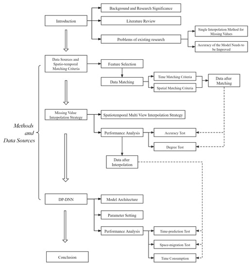
Figure 1.
Research methodology figure.
2. Methods and Data Sources
2.1. Data Sources and Spatiotemporal Matching Criteria
2.1.1. Feature Selection of Multi-Source Data
A total of 50 characteristics were selected to analyze the daily correlation between AOD and PM concentrations in the Beijing–Tianjin–Hebei–Shandong region. Table 1 shows the output and input characteristics. PM was selected as the output feature in this paper. AOD was selected as the main input feature; NDVI, meteorology, time lag, spatial identification, time node, and other features were selected as auxiliary input features.

Table 1.
Features used in the Beijing–Tianjin–Hebei–Shandong region.
2.1.2. Multiple Data Sources
(1) Overview of the study area: the Beijing–Tianjin–Hebei–Shandong area is located in the Bohai Rim region, between 34°22 N–42°40 N and 113°27 E–122°42 E, accounting for about 3.97% of the national area. It has a temperate continental monsoon climate, 39 cities, and 152 national automatic air environment quality monitoring points. With the construction of the Beijing–Tianjin–Hebei–Shandong urban agglomeration and the development of the Bohai economic circle, the geomorphic environment, and urban human activities in this area have changed, and the air quality has been affected. In order to better reflect the spatial distribution of PM concentration and its impact on human health, it is necessary to monitor the whole range of inhalable particulate matter in this area.
(2) Timespan: the data are from 1 January 2018 to 31 December 2018.
(3) Ground monitoring PM concentration data: the measured PM concentration data used are from the national urban air quality real-time release platform, and the daily air quality data of 152 national air environment quality automatic monitoring points in Beijing, Tianjin, Hebei, and Shandong were obtained. Figure 2 shows the scope of the study area and the distribution location of 152 monitoring points, including 12 in Beijing, 14 in Tianjin, 52 in Hebei Province, and 74 in Shandong Province.
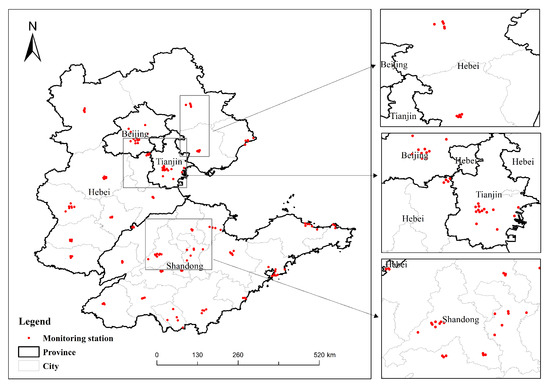
Figure 2.
Locations of air quality monitoring points of the Beijing–Tianjin–Hebei–Shandong region in 2018.
(4) MODIS AOD data: Terra/Aqua MODIS 3 km C6.1 Level 2 AOD products were downloaded from the NASA laads DAAC website. Compared with C6 version [44], version C6.1 optimizes dark blue and dark pixel algorithms and fixes algorithm defects. At the same time, a new surface reflection model was developed to eliminate the systematic deviation and improve the prediction accuracy of high altitude, rugged, and smog areas. In this study, MODIS 3 km C6.1 Level 2 AOD products covering the study area were collected, and the extracted wavelength in the Beijing–Tianjin–Hebei–Shandong area of 0.55 m AOD was used in this study.
(5) Meteorological features: the data were from the meteorological website darksky, with a spatial resolution of 0.25° × 0.25°. The near-surface meteorological data of the selected latitude and longitude can be called through the python API interface. The selected latitude and longitude coordinates can be refined to four decimal places. The data value returned by the call is the interpolation of the grid around the selected latitude and longitude. The website’s data sources [45] include 13 data sources such as NCEP (National Centers for environmental prediction) in the United States to provide global meteorological data prediction.
(6) Normalized vegetation index (NDVI): NDVI is an important parameter for detecting vegetation growth status, vegetation coverage, and radiation error. It can reflect the background impacts of the plant canopy, such as soil, wet ground, and roughness, and is related to vegetation coverage. It can not only reflect the light radiation intensity and plant growth state but the characteristics of the geographical structure of the monitoring point. We collected the NDVI products of MODIS 1 km C6 version level 3 in the study area and extracted the NDVI from the Beijing–Tianjin–Hebei–Shandong region for this study.
(7) Coordinates of monitoring points: the longitude and latitude coordinates are refined to four decimal places. The data are Beijing air quality data and from the National Urban Air Quality Real-Time Release Platform.
2.1.3. Spatiotemporal Matching of Multi-Source Heterogeneous Data
The above AOD, meteorological data, NDVI data, and measured PM concentration data near the ground were matched for subsequent modeling and analysis. The data matching follows the following criteria:
(1) Time matching. Based on PM ground monitoring points. The recording date of each data monitoring sensor shall prevail and corresponds to the data recording date of PM ground monitoring point one by one. Secondly, since the NDVI data is a 16-day product, the simple exponential smoothing method is used to expand it into the annual data.
(2) Spatial matching. Based on PM ground monitoring points. For AOD, take the longitude and latitude coordinates of 152 monitoring points as the center, take the AOD mean within 8 km as the respective results of aqua and Terra, and then take the mean of the results of aqua and Terra as the AOD value of the monitoring point. It should be noted here that 8 km is taken to avoid abnormal and missing data on longitude and latitude coordinates. At the same time, due to the bow effect during satellite scanning—as the scanning angle increases and under the influence of the curvature of the Earth, the pixel size gradually increases, resulting in geometric deformation. The geographic distance obtained after longitude and latitude conversion between pixels in the data set is greater than 3 km. Therefore, 8 km will include at least one pixel around the target location. For AODs, due to the continuous transmission and diffusion of aerosol optical thickness in geospatial space, the air quality of a location depends not only on its previous (t − 1) aerosol optical thickness but also on the air quality of its neighbors. In order to convert the air quality data with sparse spatial distribution into a consistent size for the subsequent prediction model, the AOD is spatially transformed according to the following strategies. As shown in Figure 3, taking the circular range of aerosol optical thickness at the monitoring point as the center, this paper uses and two concentric circles to divide the geospatial space into 16 adjacent areas, and the radii of the circles are 20 and 100 km. All areas are centered on the target detection station, and the area is expanding from inside to outside. In addition, different angle regions correspond to different geographical types, temporal, and spatial characteristics. In addition, this paper summarizes and averages the AOD extracted in each region, and each region has an average value. Finally, 17 AODs can be obtained, 1 from the target monitoring point, which is recorded as AOD; 16 from adjacent areas are recorded as AODs. In this study, the above spatial conversion processing was carried out for the time point of each monitoring point.
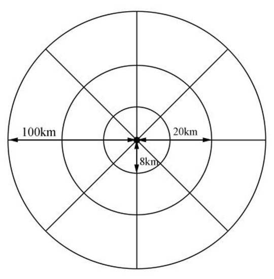
Figure 3.
Data conversion module of AODs.
The following three aspects are mainly considered in the design of the above conversion. Firstly, considering the diffusion of air pollution, the air quality data recorded by air quality monitoring points can be regarded as second-hand pollution sources due to the continuous diffusion of aerosols in geospatial space. Using these signals from spatial neighbors, the subsequent model can obtain more information. Secondly, considering the spatial correlation, the spatial division transforms the spatially scattered aerosol data into regional-level data, and the closer region has finer spatial granularity than the farther region. In addition, the influences of regions with different distances from the target are related to the distances, which follows the first law of geography [46]. Thirdly, considering the scalability of the model, spatial aggregation reduces the complexity of the model, because its input data have an upper limit to their number of regions. Moreover, spatial interpolation can generate consistent input for all regions by filling in missing values to overcome spatial sparsity. That enabled us to use the data from different sites for model training and enhance the data of the deep learning model.
(3) NDVI: Take the longitude and latitude coordinates of 152 monitoring points as the center, take the mean values of NDVI within 8 km as the results of aqua and Terra, and then take the mean value of the results of aqua and Terra as the NDVI value of the monitoring point. It should be noted that 8 km was the first to avoid data loss due to the bow effect. Secondly, NDVI data are 16-day products. If the product data are missing within the selected date, they will have a serious impact on the subsequent time matching and missing value interpolation. Therefore, expand the extraction range to improve the utilization of NDVI data.
(4) Meteorological data: Centered on the longitude and latitude coordinates of 152 monitoring points, since the precision of the coordinates that can be called by the meteorological data source is consistent with that of the longitude and latitude coordinates of the monitoring points published by the national urban air quality real-time publishing platform. The meteorological data named according to the longitude and latitude coordinates of the monitoring points can be used directly.
2.2. Missing Value Interpolation Strategy—Spatiotemporal and Multiview
2.2.1. Spatiotemporal Multiview Interpolation Strategy
The lack of data caused by monitoring sensor failure will not only affect the continuity of real-time monitoring data and the analyzability of subsequent data but also increase the complexity of model construction, which greatly interferes with the qualitative and decision-making of results. The filling of missing data is the basis of all subsequent related tasks. There are several difficulties in filling in these time-series data with geographical coordinates:
(1) The absence is basically random. In extreme cases, the loss of points will evolve into a segmental and strip-shaped loss. When the whole row and block are missing, the non-negative matrix decomposition method finds it difficult to obtain effective processing results.
(2) Spatially, the spatial weight matrix based on different types of distances will get different interpolation results. No matter which distance is used alone, the data information contained in other distances will be lost. In terms of time, the characteristics change periodically with time [37,38,39,40,41,42], and severe rain and snow will lead to large fluctuations in time series data. This special change plays a key role in subsequent data analysis, but the existing classical time series interpolation methods will smooth and distort the situation of special weather. As common interpolation methods in the field of pure space and time, although they can achieve more effective results, they will inevitably cause information loss. Therefore, it is necessary to further combine the interpolation method integrating time and space to supplement and improve the information utilization and reduce the error.
In order to solve the above problems, this paper proposes two interpolation modules: hourly mean module and spatiotemporal multiview module. When dealing with the missing data of daily observation data, first try to use the complete hourly data for interpolation, and take the 24 h data mean of the current day as the interpolation value of the missing daily observation data. If the hourly data are also missing, the spatiotemporal multi view interpolation module is used for interpolation. Next, as for the solution of spatial problems, the module includes KNN and iterative interpolation method. KNN and iterative interpolation methods obtain spatial bad weather information according to the similarity and correlation between data. Therefore, it can overcome the smooth distortion of bad weather data information caused by the linear interpolation method. Finally, the entropy weight method is used to fuse the results of the spatiotemporal multiview interpolation module.
The specific algorithms and steps of the spatiotemporal multiview interpolation module will be described in the next section.
2.2.2. Interpolation Algorithm
For each feature, the monitoring point data matrix is shown in Figure 4: m monitoring points and n continuous time points. Each row represents a monitoring point and each column represents a time point. The data of S monitoring point is missing at T time point, and the missing point is recorded as V. Similarly, we can see the missing point v.
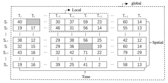
Figure 4.
Multiview interpolation module.
For the interpolation of missing point V, consider using the numerical interpolation of different adjacent monitoring points at the same time point, such as S–S, which is called spatial view in this paper. Consider using numerical interpolation at different time points of the same monitoring point, such as T–T, which is called time view in this paper. Secondly, the local and global views can be obtained for different adjacent ranges of adjacent monitoring points and different lengths of adjacent time periods: for some continuous time points, the values of some adjacent monitoring points are used for interpolation, which is called local view in this paper; if the values of all monitoring points and time points are used for interpolation, it is called global view.
This paper selects appropriate interpolation methods for different interpolation views:
(1) The time view uses exponential weighted moving average (EWMA) and polynomial interpolation to capture the time characteristics: the final prediction result is the average prediction value of EWMA and polynomial interpolation.
(2) Spatial views use inverse distance weighted (IDW) interpolation to capture spatial properties: IDW finds spatial adjacent monitoring points according to the distance between each monitoring point and the target monitoring point. Then it assigns weights to the observation data of each adjacent monitoring point according to the distance, and finally makes a weighted average of the observation data and corresponding weights of each spatial adjacent monitoring point.
(3) The local view uses the k-nearest neighbor (KNN) method to capture the proximity correlation of spatiotemporal interaction: When certain data are missing, select the same feature of spatially adjacent monitoring points (within 100 km in this paper), and select the observation data of 30 spatially adjacent time points at the same time. Calculate the mean square error between the observation data of the 30 time points of the adjacent monitoring points and the observation data of the time points with missing values, assign weights to the 30 time points based on the reciprocal of the sum of the mean square errors of the adjacent monitoring points, and make a weighted average of the data of the 30 time points of the target monitoring points.
(4) The global view uses iterative interpolation to capture the long-term regularity of spatiotemporal interaction: when a feature interpolation is performed, the features of the target monitoring points are taken as the interpreted features, the same features of the other 151 monitoring points are taken as the interpreted features, and different time points are equivalent to different samples for Iterative Regression. Among the 151 monitoring points, the higher the similarity with the target monitoring point, the greater the weight. The results of the above four methods are recorded as , , , and respectively. After the spatiotemporal multiview interpolation of all data is completed, the weight of each view is obtained by entropy weight method for the complete data of the four views, and recorded as , , , and , then the final interpolation result corresponding to each missing value is:
2.2.3. Effect Test and Results of Interpolation Algorithm
The effect of the interpolation algorithm was verified in terms of accuracy and level of completion. The results are shown in Table 2 and Table 3.
Table 2.
Interpolation accuracy test.
Table 3.
The degree of interpolation completion.
(1) Accuracy: For each feature of each monitoring point, 25% of the non-empty observation data were randomly extracted and the observation data at the corresponding position are erased to generate missing data. Then, the missing data of the erased position were interpolated, and 20 repeated experiments were carried out. The interpolation results are compared with 25% of the observed data. During the operation, the situation wherein the interpolation results cannot be generated was not counted. The evaluation indexes were relative error (RE) and mean absolute error (MAE). The units of MAE, MSE, and RMSE are g/m, g/m, and g/m, respectively.
(2) Level of completion: We used each view for interpolation, generated modeling data in 2018, and counted the deficiencies of each view before and after interpolation.
From Table 2, except for meteorological features, higher prediction accuracy can be obtained when using local and global views alone. Among them, local views are more adaptive and suitable for different feature fields. Although the error of the time view is slightly higher, the local view can not effectively interpolate the block data loss, the spatial view and global view can not effectively interpolate the strip loss, the prediction error increases, and even the interpolation results can not be generated. Therefore, this paper still retains the time view in multiple views, so as to improve the interpolation level of completion; The results in Table 2 and Table 3 confirm that multiview interpolation with a weighted combination of four views can effectively improve the accuracy and level of completion of interpolation.
Finally, 42,660 valid data were obtained, accounting for 76.9% of the sample size without deletion.
2.3. DP-DNN
2.3.1. DP-DNN Model Architecture
The main features and auxiliary features will have different effects on future air quality. In most cases, all auxiliary features will determine the development environment and space of the main features at the same time. Secondly, each auxiliary feature will act on the main feature separately to affect the future air quality. At the same time, considering the lag effect of features and the inconsistency of correlations and partial correlation between features in different fields, the conventional depth neural network model finds it difficult to effectively predict the concentration of PM. In order to capture the individual and overall impact (collectively referred to as high-order characteristics), DP-DNN architecture includes seven neural network modules, so that the main features are fused in parallel, and each auxiliary feature is fused to capture high-order characteristics, and the final result is obtained by linear fusion of output. The reason for distinguishing features is that the main features and prediction targets come from the same field, and the auxiliary features and prediction targets come from different fields. DP-DNN emphasizes the main features and captures the influence of each auxiliary feature on the main features, so as to learn the high-order characteristics between various features.
This paper specifies AOD as the main input feature; and AODs, NDVI, meteorology, time lag, time node, and spatial identification as the auxiliary input features. The seven modules are:
(1) Spatial pollution linkage module: Used to capture the spatial diffusion and spatial correlation of pollution. After AOD and AODs are input into the module, the space pollution linkage module can be obtained.
(2) Vegetation index module: Used to capture the background impacts of plants, such as soil, vegetation cover, etc. It can not only reflect the light radiation intensity and plant growth state but also serve as the characteristics of the geographical environment structure of the monitoring point.
(3) Time delay meteorological module, meteorological module: Used to capture the impacts of historical and current meteorological conditions on direct characteristics. The reason why this paper establishes two modules is that there are historical weather data and current day data. This paper believes that the impacts of historical and current-day data are different and complex, and the weather conditions of the previous day will affect the weather conditions of the next day. The weather, wind speed, wind direction, humidity, and air pressure are regarded as the characteristics of historical and current meteorological condition data. After inputting the historical and current weather conditions into the module together with AOD, two modules can be obtained, namely, the meteorological module and the time-delay meteorological module.
(4) Time node module and space identification module: Used to simulate the impact of time and space terrain on air quality. Specifically, time characteristics (current month) are used to simulate the law of air quality in the time dimension. For example, due to heating, winter always has higher AOD and PM concentrations than summer. In addition, this paper uses station longitude and latitude to simulate the impact of terrain and air quality. For example, the air quality of artificial gathering areas and commercial areas is generally worse than that of park and forest land. By fusing aerosol data with time and space identification respectively, the time node module and space identification module can be obtained.
(5) All feature fusion modules: Except for individual influence, all indirect features will act on direct features at the same time, thereby affecting the development environment of air quality. In order to capture the impact of this integrity, we designed an all-feature fusion module, which inputs all direct and indirect features into the module.
Finally, the seven captured high-order characteristics are connected through the splicing layer, and the weighted combination based on leakyrelu activation function is used to simulate these dynamic effects and produce the final prediction. The model flow is shown in Figure 5.
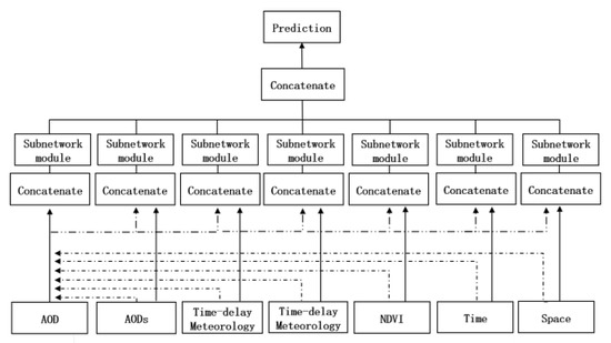
Figure 5.
Flow diagram of DP-DNN algorithm.
2.3.2. DP-DNN Model Algorithm Architecture
As the input of each fusion is more than two, and it is impossible to perform operations such as point multiplication and addition, DP-DNN combines the input features by using a splicing layer, so as to fuse all different features. Then, multiple fully connected layers are used to learn the high-order characteristics between features in a nonlinear way. In order to better train the neural network, some residual full connection layers are added between the full connection layers. By connecting the full connection layer and the residual, the residual full connection layer can easily transfer the previous information to the later network through a jump transmission mode, which can effectively solve the problems of gradient disappearance, network degradation, and so on. Add a dropout layer in the module to prevent the model from overfitting (a. linear part: . b. nonlinear part: ). The module architecture is shown in Figure 6.
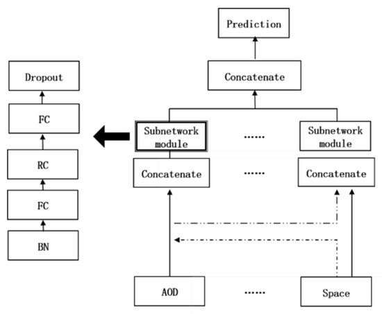
Figure 6.
Module architecture. of DP-DNN.
2.3.3. Feature Transformation and Standardization
The classification features and string features are processed by feature engineering, and the features are extracted from the original data to the greatest extent for the use of algorithms and models, so as to capture the dependencies between features and learn the internal dynamics of each influencing feature. Feature engineering can transform classification features and string features into vectors of real values, and capture the similarity between different categories. In this paper, time node features and spatial identification features are processed by feature engineering, respectively, in order to capture the interaction with AOD in DP-DNN.
Before feature fusion learning, the original numerical data are standardized [47]. This paper adopts the method of adjusting the distribution of input features to the standard normal distribution with a mean value of 0 and a variance of 1 to standardize the input features, which can enhance the robustness of input features, avoid the problem of gradient disappearance and speed up the training speed.
2.3.4. DP-DNN Model Parameter Setting
The appropriate number of layers and neurons is the basis for the excellent performance of DP-DNN. After tuning, for each module, we started with a full connection layer with a size of 24, connected a residual connection layer with a size of 24, added a full connection layer with a size of 12 and a dropout layer with a rate = 0.01, and finally added two full connection layers with sizes of 8 and 4, respectively. For the high-order feature fusion layer, it was composed of a full connection layer with a size of 8 and a residual connection layer, a dropout layer with a rate = 0.01, and a full connection layer with a size of 4. Finally, the result is output through the activation function leakyrelu. The activation functions used in the full connection layer are leakyrelu; In order to prevent overfitting of the model, the L2 regularization standard with the weight of 0.01 was used. The optimization function compiled by the model used the Adam function with a learning rate of 0.01, the batch size was 5120, and the number of epochs was set to 20.
3. Research Results
Using the effective data of 152 monitoring points in the four regions of Beijing, Tianjin, Hebei, and Shandong in 2018 as the experimental data, the DP-DNN was trained with the help of the backpropagation training method to minimize the average absolute error between the predicted values and the ground values. In order to verify the prediction accuracy, the samples were randomly divided 100 times, and the error mean was used for model evaluation. In order to test the ability of time prediction and spatial migration of the model, the training set and test set were divided as follows:
(1) Time prediction: We use the data of all monitoring points to randomly divide the data by month so that the sample ratio of the training set to test set was 3:1;
(2) Regional migration: Using the data of 2018, 152 monitoring points were randomly sampled to make the sample ratio of the training set to test set 3:1;
(3) Evaluation index: The mean values of the mean absolute error (MAE), relative error (RE), mean square error (MSE), and root mean square error (RMSE) of 100 experiments were used to evaluate the simulation results of the model:
where is the true value of the i-th sample in the j-th experimental verification set, is the predicted value of the i-th sample in the j-th experimental verification set, and N is the sample size of the verification set. For a more intuitive comparison model, the following common models are selected for comparison with the models used in this paper.
(1) MLP (multilayer perceptron): Follows DP-DNN “all feature modules”, and the model details were set with reference to DP-NN. The (1 and 2) model was introduced to verify the necessity of DP-DNN multi-module architecture through error comparison.
(2) Multiple input neural network (MI-NN): It imitates DP-DNN, but does not distinguish between main features and auxiliary features. Each module captures the individual characteristics of each type of feature, rather than the interaction characteristics with AOD. Finally, the results were output through the activation function leakyrelu, and other model details were set with reference to DP-NN.
(3) Long short term memory (LSTM): Improved from the cyclic neural network (RNN) model, it is a special recursive neural network, which uses a gating mechanism to capture long-term dependence. As LSTM has strict requirements on data integrity, the input features here were PM concentration, AOD, AODs, time node, and spatial identification.
(4) Geographically weighted region (GWR): A geographically weighted model combined with the automatic search of the optimal bandwidth was adopted. When GWR processes more input features, huge time overheads are incurred in the selection of the optimal bandwidth and model fitting. Therefore, the features used were AOD, time node, and spatial identification.
(5) Boosting orthogonal least squares regression (B-olsr): The least-squares linear regression model combined with boosting was adopted [48]. As it is difficult to deal with a large number of discrete characteristics, the monitoring points were divided and classified according to their provinces when using the model. We classified the months by quarter for dimensionality reduction.
(6) Elastic network (EN): Improved from the lasso model and ridge regression model; it is a continuous iterative regression analysis method.
Figure 7 and Figure 8 are, respectively, the error line graphs of the space-migration test and the time prediction test. The detailed error results are shown in the Table 4.
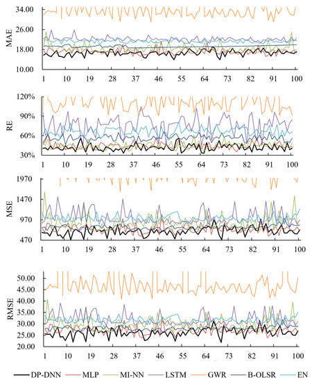
Figure 7.
Error line charts of PM concentration—regional migratory prediction based the Beijing–Tianjin–Hebei–Shandong Region in 2018.
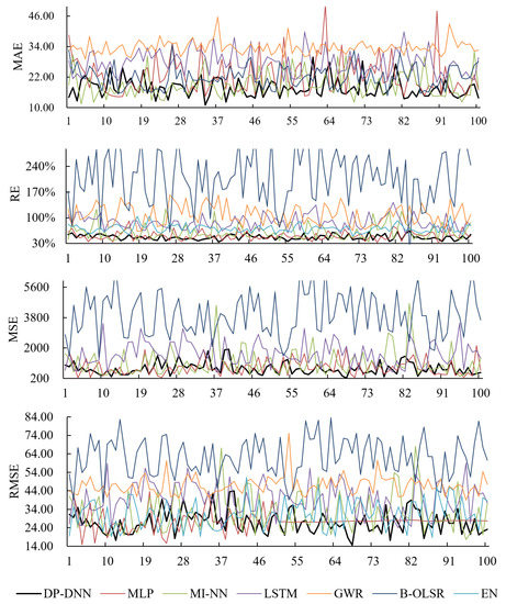
Figure 8.
Error line charts of PM concentration—regional time prediction based on the Beijing–Tianjin–Hebei–Shandong region in 2018.
Table 4.
Error and time cost of PM concentration prediction based the Beijing–Tianjin–Hebei–Shandong region in 2018.
The B-olsr model finds it difficult to deal with a sparse matrix with many discrete characteristics. Although the prediction stability was good in the random monitoring point experiment, the error fluctuates greatly in the time prediction test; EN could effectively deal with the expansion of dimension through penalty term, but the prediction accuracy was poor. The generalization ability of GWR was lower than that of neural network model, and the error fluctuation in regional migration prediction increased significantly. From the perspective of GWR calculation speed, the calculation process for large-scale samples is cumbersome, and it takes a long time to find the optimal bandwidth and model fitting. From the error results of many experiments, the LSTM model has strong stability, but compared with DP-DNN, the error is large and the model takes too long. Although MI-NN and MLP models are slightly ahead of DP-DNN in speed, the accuracies of MAE, RE, MSE, and RMSE are lower than that of DP-DNN. From the chart, DP-DNN also has good stability and short-term prediction ability. At the same time, it also proves that the DP-DNN model can indeed capture more data information through multi-module structure.
DP-DNN can effectively deal with high-dimensional features and capture the complex relationship between features. It shows good universality and robustness in the research of dealing with complex atmospheric environmental pollution. Compared with the benchmark model, DP-DNN has finer feature granularity, higher-order feature characteristics, more reasonable network architecture, and faster update frequency. DP-DNN has excellent short-term spatiotemporal migration prediction accuracy and stability, and good computing speed to meet the needs of practical applications. DP-DNN is an effective means for completing historical pollutant data and predicting future pollutant concentration and current pollutant concentration in areas without monitoring points.
4. Conclusions and Prospect
Aiming at the problems of missing historical data of PM concentration and small coverage of monitoring points, we integrated multi-source data such as NASA aerosol optical thickness and constructed and interpolated the missing values using a spatiotemporal multiview interpolation model, which made up for the information loss caused by a single interpolation method. Among them, AOD and AODs complete the interpolation of all missing values. Finally, the established DP-DNN improved the data utilization and PM concentration prediction accuracy. While the calculation speed is excellent, the short-term prediction results of the model are the most stable. The constructed DP-DNN model can return a 3 km resolution to the given latitude and longitude. The predicted PM concentration with a 3 km high spatial resolution has a good application potential. The PM concentration data estimated based on this method can be further applied to the fields of medicine, public health, economics, and sociology. For example, we estimated the historical long term PM concentration time series data of a place where patients were to be studied and combined the data with health effects indicators such as the incidence rates, mortality rates, and outpatient rates of specific diseases to study the chronic health effects, which provided evidence for the long-term relationship between PM exposure and disease. We estimated the annual average concentration of historical PM in the province and established an econometric model in combination with the data in the Statistical Yearbook, which can be used to analyze the promotion of urbanization, the development of urban agglomeration, the effectiveness of changing the mode of economic development, and other issues.
Author Contributions
J.L. and Y.S. set up the problem and computed the details. Q.L. polished the draft. All authors have read and agreed to the published version of the manuscript.
Funding
National Social Science Foundation of China (21ZD081 and 21ZDA014).
Institutional Review Board Statement
Not applicable.
Informed Consent Statement
Not applicable.
Data Availability Statement
Not applicable.
Conflicts of Interest
The authors declare no conflict of interest.
References
- Geng, G.; Zhang, Q.; Martin, R.V.; van Donkelaar, A.; Huo, H.; Che, H.; Lin, J.; He, K. Estimating long-term PM2.5, concentrations in China using satellite-based aerosol optical depth and a chemical transport model. Remote Sens. Environ. 2015, 166, 262–270. [Google Scholar] [CrossRef]
- Lee, D.; Mukhopadhyay, S.; Rushworth, A.; Sahu, S.K. A rigorous statistical framework for spatio-temporal pollution prediction and estimation of its long-term impact on health. Biostatistics 2017, 18, 370–385. [Google Scholar] [CrossRef] [PubMed][Green Version]
- Mukhopadhyay, S.; Sahu, S.K. A Bayesian spatiotemporal model to estimate long-term exposure to outdoor air pollution at coarser administrative geographies in England and Wales. J. R. Stat. Soc. Ser. A Stat. Soc. 2018, 181, 465–486. [Google Scholar] [CrossRef]
- Fang, X.; Zou, B.; Liu, X.; Sternberg, T.; Zhai, L. Satellite-based ground PM2.5 estimation using timely structure adaptive modeling. Remote Sens. Environ. 2016, 186, 152–163. [Google Scholar] [CrossRef]
- Van Donkelaar, A.; Martin, R.V.; Brauer, M.; Hsu, N.C.; Kahn, R.A.; Levy, R.C.; Lyapustin, A.; Sayer, A.M.; Winker, D.M. Global Estimates of Fine Particulate Matter using a Combined Geophysical-Statistical Method with Information from Satellites, Models, and Monitors. Environ. Sci. Technol. 2016, 50, 3762–3772. [Google Scholar] [CrossRef]
- He, Q.Q.; Huang, B. Satellite-based mapping of daily high-resolution ground PM2.5 in China via space-time regression modeling. Remote Sens. Environ. 2018, 206, 72–83. [Google Scholar] [CrossRef]
- Wang, Z.; Chen, L.; Tao, J.; Zhang, Y.; Su, L. Satellite-based estimation of regional particulate matter (PM) in Beijing using vertical-and-RH correcting method. Remote Sens. Environ. 2010, 114, 50–63. [Google Scholar] [CrossRef]
- Fu, D.; Xia, X.; Wang, J.; Zhang, X.; Li, X.; Liu, J. Synergy of AERONET and MODIS AOD products in the estimation of PM2.5 concentrations in Beijing. Sci. Rep. 2018, 8, 10174. [Google Scholar] [CrossRef]
- Wang, J.; Christopher, S.A. Intercomparison between satellite-derived aerosol optical thickness and PM2.5 mass: Implications for air quality studies. Geophys. Res. Lett. 2003, 30, 2095–2098. [Google Scholar] [CrossRef]
- Engel-Cox, J.A.; Holloman, C.H.; Coutant, B.W.; Hoff, R.M. Qualitative and quantitative evaluation of MODIS satellite sensor data for regional and urban scale air quality. Atmos. Environ. 2004, 38, 2495–2509. [Google Scholar] [CrossRef]
- Jia, S.; Su, L.; Tao, J.; Wang, Z.; Chen, L.; Shang, H. A study of multiple regression method for estimating concentration of fine particulate matter using satellite remote sensing. China Environ. Sci. 2014, 34, 565–573. [Google Scholar]
- Zang, Z.; Wang, W.; Cheng, X.; Yang, B.; Pan, X.; You, W. Effects of Boundary Layer Height on the Model of Ground-Level PM2.5 Concentrations from AOD: Comparison of Stable and Convective Boundary Layer Heights from Different Methods. Atmosphere 2017, 8, 104. [Google Scholar] [CrossRef]
- Gupta, P.; Christopher, S.A. Particulate matter air quality assessment using integrated surface, satellite, and meteorological products: Multiple regression approach. J. Geophys. Res. Atmos. 2009, 114, 1–13. [Google Scholar] [CrossRef]
- Koelemeijer, R.B.A.; Homan, C.D.; Matthijsen, J. Comparison of spatial and temporal variations of aerosol optical thickness and particulate matter over Europe. Atmos. Environ. 2006, 40, 5304–5315. [Google Scholar] [CrossRef]
- Chen, H.; Li, Q.; Zhang, Y.H.; Zhou, C.Y.; Wang, Z. Estimations of PM2.5 concentrations based on the method of geographical weighted regression. Acta Sci. Circumstantiae 2016, 36, 2142–2151. [Google Scholar]
- He, Q.Q.; Huang, B. Satellite-based high-resolution PM2.5, estimation over the Beijing-Tianjin-Hebei region of China using an improved geographically and temporally weighted regression model. Environ. Pollut. 2018, 236, 1027–1037. [Google Scholar] [CrossRef] [PubMed]
- Chen, H.; Li, Q.; Wang, Z.; Sun, Y.; Mao, H.; Cheng, B. Utilization of MERSI and MODIS data to monitor PM2.5 concentration in Beijing–Tianjin–Hebei and its surrounding areas. J. Remote Sens. 2018, 22, 114–124. [Google Scholar]
- Jiang, M.; Sun, W.; Yang, G.; Zhang, D. Modelling Seasonal GWR of Daily PM2.5 with Proper Auxiliary Variables for the Yangtze River Delta. Remote Sens. 2017, 9, 346. [Google Scholar] [CrossRef]
- Wu, J.S.; Yao, F.; Li, W.F.; Si, M. VIIRS-based remote sensing estimation of ground-level PM2.5 concentrations in Beijing–Tianjin–Hebei: A spatiotemporal statistical model. Romote Sens. Environ. 2016, 184, 316–328. [Google Scholar] [CrossRef]
- Wu, Y.; Guo, J.; Zhang, X.; Tian, X.; Zhang, J.; Wang, Y.; Duan, J.; Li, X. Synergy of satellite and ground based observations in estimation of particulate matter in eastern China. Sci. Total Environ. 2012, 433, 20–30. [Google Scholar] [CrossRef]
- Yao, L.; Lu, N. Spatiotemporal distribution and short-term trends of particulate matter concentration over China, 2006–2010. Environ. Sci. Pollut. Res. 2014, 21, 9665–9675. [Google Scholar] [CrossRef] [PubMed]
- Shao, Q.; Chen, Y.; Li, J. Inversion of PM2.5 Concentration in Beijing Based on Satellite Remote Sensing and Meteorological Reanalysis Data. Geogr. Geo-Inf. Sci. 2018, 34, 38–44. [Google Scholar]
- Zou, B.; Chen, J.; Zhai, L.; Fang, X.; Zheng, Z. Satellite Based Mapping of Ground PM2.5 Concentration Using Generalized Additive Modeling. Remote Sens. 2016, 9, 1. [Google Scholar] [CrossRef]
- Kloog, I.; Koutrakis, P.; Coull, B.A.; Lee, H.J.; Schwartz, J. Assessing temporally and spatially resolved PM2.5 exposures for epidemiological studies using satellite aerosol optical depth measurements. Atmos. Environ. 2011, 45, 6267–6275. [Google Scholar] [CrossRef]
- Sorek-Hamer, M.; Strawa, A.W.; Chatfield, R.B.; Esswein, R.; Cohen, A.; Broday, D.M. Improved retrieval of PM2.5 from satellite data products using non-linear methods. Environ. Pollut. 2013, 182, 417–423. [Google Scholar] [CrossRef]
- Li, T.; Shen, H.; Zeng, C.; Yuan, Q.; Zhang, L. Point-surface fusion of station measurements and satellite observations for mapping PM2.5 distribution in China: Methods and assessment. Atmos. Environ. 2017, 152, 477–489. [Google Scholar] [CrossRef]
- Lyu, H.; Dai, T.; Zheng, Y.; Shi, G.; Nakajima, T. Estimation of PM2.5 Concentrations over Beijing with MODIS AODs Using an Artificial Neural Network. Sci. Online Lett. Atmos. 2018, 14, 14–18. [Google Scholar]
- Zou, B.; Wang, M.; Wan, N.; Wilson, J.G.; Fang, X.; Tang, Y. Spatial modeling of PM2.5 concentrations with a multifactoral radial basis function neural network. Environ. Sci. Pollut. Res. Int. 2015, 22, 395–404. [Google Scholar] [CrossRef]
- Yao, L.; Lu, N.; Jiang, S. Artificial Neural Network (ANN) for Multi-source PM2.5 Estimation Using Surface, MODIS, and Meteorological Data. In Proceedings of the 2012 International Conference on Biomedical Engineering and Biotechnology, Macau, Macao, 28–30 May 2012; pp. 1228–1231. [Google Scholar]
- Mei, B.; Tian, M. Analysis of Influential Factors on PM2.5 in Beijing Based on Spatio-Temporal Model. J. Appl. Stat. Manag. 2018, 37, 571–586. [Google Scholar]
- Ellett, F.S.; Ericson, D. Correlation, partial correlation, and causation. Synthese 1986, 67, 157–173. [Google Scholar] [CrossRef]
- Wang, W.; Zhao, S.; Jiao, L.; Taylor, M.; Zhang, B.; Xu, G.; Hou, H. Estimation of PM2.5 Concentrations in China Using a Spatial Back Propagation Neural Network. Sci. Rep. 2019, 9, 13788. [Google Scholar] [CrossRef]
- Wang, X.Q.; Wang, F.; Jia, L.L.; Ding, Y. Retrieval and Validation of Aerosol Optical Depth by using GF-1 WFV Cameras Data. Adv. Space Res. 2020, 65, 997–1007. [Google Scholar] [CrossRef]
- Yu, W.; Nan, Z.; Wang, Z.; Chen, H.; Wu, T.; Zhao, L. An Effective Interpolation Method for MODIS Land Surface Temperature on the Qinghai–Tibet Plateau. IEEE J. Sel. Top. Appl. Earth Obs. Remote Sens. 2015, 8, 4539–4550. [Google Scholar] [CrossRef]
- Safarpour, S.; Abdullahb, K.; Limb, H.S.; Dadrasa, M. Spatial Interpolation of Aerosol Optical Depth Pollution: Comparison of Methods for the Development of Aerosol Distribution. ISPRS Int. Arch. Photogramm. Remote Sens. Spat. Inf. Sci. 2017, 4, 237–244. [Google Scholar] [CrossRef]
- Sathe, Y.; Kulkarni, S.; Gupta, P.; Kaginalkar, A.; Islam, S.; Gargava, P. Application of Moderate Resolution Imaging Spectroradiometer (MODIS) Aerosol Optical Depth (AOD) and Weather Research Forecasting (WRF) model meteorological data for assessment of fine particulate matter (PM2.5) over India. Atmos. Pollut. Res. 2019, 10, 418–434. [Google Scholar] [CrossRef]
- Beckerman, B.S.; Jerrett, M.; Serre, M.; Martin, R.V.; Lee, S.J.; Van Donkelaar, A.; Ross, Z.; Su, J.; Burnett, R.T. A hybrid approach to estimating national scale spatiotemporal variability of PM2.5 in the contiguous United States. Environ. Sci. Technol. 2013, 47, 7233–7241. [Google Scholar] [CrossRef] [PubMed]
- Chow, J.C.; Chen, L.W.; Watson, J.G.; Lowenthal, D.H.; Magliano, K.A.; Turkiewicz, K.; Lehrman, D.E. PM2.5 chemical composition and spatiotemporal variability during the California Regional PM10/PM2.5 Air Quality Study (CRPAQS). J. Geophys. Res. Atmos. 2006, 111, 1–17. [Google Scholar] [CrossRef]
- Lin, G.; Fu, J.; Jiang, D.; Hu, W.; Dong, D.; Huang, Y.; Zhao, M. Spatio-temporal variation of PM2.5 concentrations and their relationship with geographic and socioeconomic factors in China. Int. J. Environ. Res. Public Health 2013, 11, 173–186. [Google Scholar] [CrossRef]
- Gelencsér, A.; May, B.; Simpson, D.; Sánchez-Ochoa, A.; Kasper-Giebl, A.; Puxbaum, H.; Caseiro, A.; Pio, C.; Legrand, M. Source apportionment of PM2.5 organic aerosol over Europe: Primary/secondary, natural/anthropogenic, and fossil/biogenic origin. J. Geophys. Res. Atmos. 2007, 112, 1–12. [Google Scholar] [CrossRef]
- Liu, Y.; Paciorek, C.J.; Koutrakis, P. Estimating regional spatial and temporal variability of PM2.5 Concentrations using satellite data, meteorology, and land use information. Environ. Health Perspect. 2009, 117, 886–892. [Google Scholar] [CrossRef]
- Kloog, I.; Nordio, F.; Coull, B.A.; Schwartz, J. Incorporating local land use regression and satellite aerosol optical depth in a hybrid model of spatiotemporal PM2.5 exposures in the Mid-Atlantic states. Environ. Sci. Technol. 2012, 46, 11913–11921. [Google Scholar] [CrossRef] [PubMed]
- National Oceanic and Atmospheric Administration Weather Prediction Center. The Heat Index Equation. Available online: http://www.wpc.ncep.noaa.gov/html/heatindex_equation.shtml (accessed on 28 May 2014).
- National Aeronautics and Space Administration. MODIS Standard Collection 6.1 Update Executive Summary. Available online: https://atmosphere-imager.gsfc.nasa.gov/documentation/collection-61 (accessed on 9 August 2017).
- Dark Sky Docs: Data Sources. Available online: https://darksky.net/dev/docs/sources (accessed on 4 September 2019).
- Tobler, W.R. A Computer Movie Simulating Urban Growth in the Detroit Region. Econ. Geogr. 1970, 46, 234–240. [Google Scholar] [CrossRef]
- Swami, A.; Jain, R. Scikit-learn: Machine Learning in Python. J. Mach. Learn. Res. 2012, 12, 2825–2830. [Google Scholar]
- Wang, X.X.; Brown, D.J. Boosting Orthogonal Least Squares Regression. Lect. Notes Comput. Sci. 2004, 3177, 678–683. [Google Scholar]
Publisher’s Note: MDPI stays neutral with regard to jurisdictional claims in published maps and institutional affiliations. |
© 2021 by the authors. Licensee MDPI, Basel, Switzerland. This article is an open access article distributed under the terms and conditions of the Creative Commons Attribution (CC BY) license (https://creativecommons.org/licenses/by/4.0/).