Article

Determining Hydrological Variability Using a Multi-Catchment Model Approach for the Western Cape, South Africa

1
Stellenbosch University Water Institute, Stellenbosch University, Private Bag X1, Matieland 7602, South Africa
2
School for Climate Studies, Stellenbosch University, Private Bag X1, Matieland 7602, South Africa
3
Global Change Biology Group, Department of Botany and Zoology, Stellenbosch University, Private Bag X1, Matieland 7602, South Africa
4
Department of Geoinformation Science, Friedrich Schiller University Jena, Loebdergraben 32, 07743 Jena, Germany
5
Southern African Science Service Centre for Climate Change and Adaptive Land Management (SASSCAL), Windhoek 10005, Namibia
*
Author to whom correspondence should be addressed.
Sustainability 2021, 13(24), 14058; https://doi.org/10.3390/su132414058
Submission received: 19 November 2021 / Revised: 10 December 2021 / Accepted: 14 December 2021 / Published: 20 December 2021

Abstract

:
Understanding the impacts of climate change requires the development of hydrological modelling tools. However, data scarcity hinders model application, performance, process simulation and uncertainty, especially for Sub-Saharan Africa. In this study, a multi-catchment approach was used to assess hydrological process variability in the Western Cape (WC) of South Africa using the JAMS/J2000 rainfall–runoff model and a Monte Carlo analysis (MCA). Due to much steeper slopes and lower evapotranspiration, the models suggest that WC is dominated by surface runoff from mountainous regions and regional groundwater flow. The results highlight the impact of the catchment size, availability and position of hydroclimatic and anthropogenic factors and the frequency of the signal-to-noise ratio (water balance). For large catchments (>5000 km2), the calibration was able to achieve a Nash–Sutcliffe efficiency (NSE) of 0.61 to 0.88. For small catchments (<2000 km2), NSE was between 0.23 to 0.39. The large catchments had an overall surface runoff, interflow and baseflow contribution of 44, 19 and 37%, respectively, and lower overall uncertainty. The simulated flow components for the small catchments were variable and these results are less certain. The use of a multi-catchment approach allows for identifying the specific factors impacting parameter sensitivities and in turn provides a means to improve hydrological process simulation.

1. Introduction

Climate change is altering the distribution and nature of precipitation patterns around the world, driving hydrological change and exacerbating the loss of natural ecosystems [1]. As a consequence, hydrological flows are projected to change on a global scale [2,3], with changes in streamflow patterns and expected alterations to the flow components thereof (surface runoff, interflow and baseflow). Naturally, these flow components are subject to seasonal variations, but during periods of peak or high flow, surface runoff and interflow are often more significant [4], while during periods of low flow, baseflow is more dominant [5]. The proportion of these flow components additionally depends on climate, land use, surface terrain, subsurface conditions and drainage characteristics [6], as well as anthropogenic water use [7]. Together, these factors control streamflow characteristics, which are spatially variable and dependent on the storage dynamics between the saturated and unsaturated zones, as well as feedback loops and dependencies within different hydrological processes and features [8]. As a result, determining hydrological component variability is necessary in climate change-related assessments and to consider dominant flow generation mechanisms.
Mountainous regions often receive the bulk of precipitation due to orographic effects and experience lower evapotranspiration [9,10]. In addition, they are often characterized by shallow soils and fractured bedrock and, as a result, are critical for groundwater recharge and river baseflow generation, as well as surface runoff contributions [11,12]. In contrast, and depending on the microtopography, the runoff response in catchment valleys is often dampened by evapotranspiration, thick unsaturated zones, river seepage and interactions with the alluvial aquifer system, and, as a result, they are sources of interflow or sub-surface runoff [13,14,15]. While spatial differences in climate directly affect rainfall–runoff response and hydrological processes, they also contribute further to changes in biophysical characteristics, such as vegetation growth and dominant groundwater flow paths, as well as geomorphological processes, such as soil formation and weathering [16], impacting streamflow dynamics. These variations can be more pronounced in semi-arid environments, where the climate is heterogenous, generating microclimates [17] in which streamflow can be spatially variable [18]. Due to these complexities, constraining hydrological component variability using models is difficult and dependent on a number of factors. Relevant hydroclimatic and biophysical data, system and process understanding that include the impact of human activities on the landscape, as well as internal model structure and variables, are needed in hydrological model applications.
The Western Cape (WC) province of South Africa, located within mediterranean southern Africa, has recently experienced a drought (2015–2018), which resulted in reservoir levels dropping to a low of 17% of their full capacity [19]. The drought has highlighted the vulnerability of the centralized water supply systems currently in use in the WC and the need for a consensus on the impact of future climate change [20]. The area lacks the hydrological modelling tools required for climate change-based assessments, as the availability of gauging meteorological and streamflow networks hinders model applications in the WC, as well as in much of southern Africa. With the improvement in remote sensing, scientific data portals [21,22] and the accessibility of data from the World Meteorological Organisation [23], rainfall–runoff models that simulate hydrological processes and flow components can be applied. However, simulations are influenced by catchment size and the availability of relevant streamflow and meteorological data, as well as streamflow characteristics and anthropogenic factors.
In this study, the distributed, process-based J2000 rainfall–runoff model was used to determine hydrological variability in the Western Cape using a multi-catchment approach that included five adjacent catchments (Verlorenvlei, Berg, Eerste, Breede and Bot River) in the WC. The climate in mediterranean South Africa is heterogenous where the flow is mainly controlled by headwater processes, resulting in different streamflow characteristics across these catchments. Although physical inputs (e.g., climate, topography, soil, hydrogeology and land use) are included as spatial inputs for distributed rainfall–runoff models (e.g., SWAT [24] and J2000 [25]), the availability of relevant data varies between each catchment. Furthermore, conceptual and empirical parameters still require calibration within rainfall–runoff models to simulate hydrological processes. To understand the impact of different parameters on the simulated hydrological processes for each catchment, a Monte Carlo analysis (MCA) was performed. With the necessity of using rainfall–runoff models for predictions of water availability in the perspective of climate change, understanding hydrological variability is required for the development of regional hydrological modelling tools. These tools are further required in early warning forecasting systems and for water management, as well as in riverine and ecosystem assessments.

2. Materials and Methods

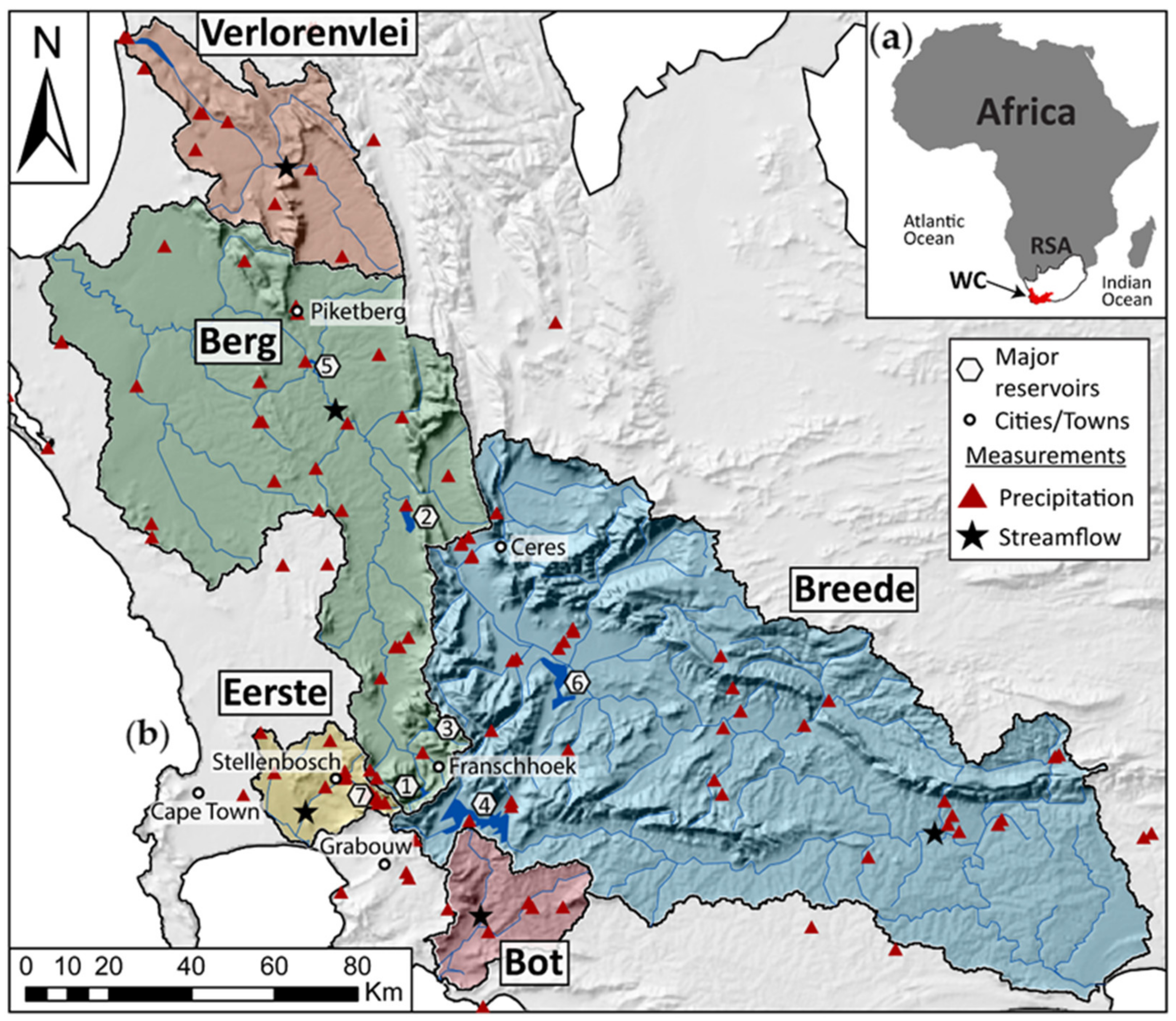
2.1. Environmental Setting

Verlorenvlei, Berg, Eerste, Bot and Breede are catchments located in the Western Cape province, covering the southernmost tip of Africa (Figure 1). These catchments range in size from relatively small, such as Eerste, Bot and Verlorenvlei (620, 864 and 1832 km2) and moderate to relatively large, such as Berg and Breede (7704 and 12,526 km2) (Table 1). Mountainous areas near the towns of Piketberg, Franshhoek, Stellenbosch, Grabouw and Ceres form the catchment headwaters, after which the catchments grade into relatively low-lying flat regions before the river systems flow into the ocean (Figure 1b).

2.1.1. Climate

The catchments under study experience mediterranean climate conditions, where the catchments have been categorized as winter rainfall zones (WRZ) [29] (Table 1). Together, the catchments comprise 31% of the parts of the Western Cape that predominately receive winter precipitation. The maximum elevation in each catchment is 2232, 2062, 1511, 1446 and 1187 m a.s.l. and the maximum yearly precipitation is on average 3198, 3053, 2067, 1143 and 556 mm as a result (Figure 2) [30]. Mean annual precipitation (MAP) for each of the study catchments is 694, 552, 487, 429 and 334 mm for Eerste, Bot, Berg, Breede and Verlorenvlei, respectively [30].
The mean daily temperature for these catchments combined is 19–21 °C for summer (DJF), 16–20 °C for autumn (MAM), 10–12 °C for winter (JJA) and 13–18 °C for spring (SON) [26]. Potential evaporation (PET) is spatially variable and ranges from 1806 to 2313 mm/yr. across the catchments (Table 1). For Berg and Verlorenvlei, mean PET exceeds 2000 mm/yr., while for Breede, Berg and Eerste, it is between 1800 and 1915 mm/yr.) [26].

2.1.2. Hydrology and Water Management

While the Verlorenvlei and Berg catchments drain towards the west into the Atlantic Ocean, Eerste, Bot and Breede drain towards the east into the Indian Ocean. Estuaries are present at each of the catchment outlets, which include (1) Velorenvlei, (2) Berg River Estuary, (3) Eerste River Estuary, (4) Botrivervlei and (5) Breede River Estuary. Verlorenvlei and Botrivervlei are of global importance (Ramsar no. 525 and 2291), but all of these estuaries have both local and national importance [31]. While these catchments support ecologically significant regions, small farm dams and water supply holding dams, as well as major reservoirs, impact downstream river flows. Reservoirs in the Berg and Breede catchments account for 58% of the total surface water supply for the City of Cape Town (COCT), which includes (1) the Berg River dam (130 Mm3), (2) Voëlvlei (164 Mm3), (3) Wemmershoek (58 Mm3) in the Berg River and (4) Theewaterskloof (480 Mm3) in the Breede. Other major reservoirs, such as (5) Miverstand (8 Mm3) and (6) Greater Brandvlei (459 Mm3), are not included in the COCT water supply, but are required for nearby towns and irrigation.

2.1.3. Geology and Hydrogeology

The study catchments fall within the Cape Fold Belt, a thrust belt which impacted the formation of a sequence of sedimentary rock layers known as the Cape Supergroup [32]. The study catchments host three major rock units. In order of ascending ages, the oldest of these formations is the Neoproterozoic Malmesbury Group (MG), which is composed of greywacke, sercitic schist, quartzite, conglomerate and limestone [33]. These rocks form a secondary fractured rock aquifer with limited primary porosity and have significant outcrops in Verlorenvlei and Berg. The MG rocks have been intruded upon by the Cambrian Cape Granite Suite, which are composed of several late-Precambrian granitoids. Although drilling indicates their presence at depth in all of the study catchments, outcrops in the Eerste are common. The Cambrian Table Mountain Group (TMG) overlies both the Malmesbury Group and the Cape Granite Suite and is only superseded in age by the Bokkeveld Group (CSG). The TMG is composed mostly of Peninsula, Graafwater and Piekenierskloof formations, which vary in thickness, but dominate the mountainous regions in the study catchments [33]. While the TMG forms a secondary fractured rock aquifer unit, it also plays host to a number of springs at formation contact points. An alluvial aquifer system, which has primary porosity, is also a common feature in all these study catchments. It varies in thickness, but is generally between 10 and 15 m thick [34].

2.1.4. Vegetation and Land Use

The Greater Cape Floristic Region, composed primarily of Fynbos, Renosterveld and Succulent Karoo shrublands are the major natural vegetation types found in the study catchments. All of these shrubland types are endemic to the mediterranean regions of the Western and Eastern Cape. While comprising several endemic plant families, common genera include Protea and Leucospermum, which are more frequently known as ‘pincushions’ and ‘Leucadendron’ (‘cone bushes’). Although these catchments are biodiversity hotspots [35,36], significant areas of land (including almost all Renosterveld) have been cleared for agricultural production since the early 2000s, with large areas of cultivated fields and viticulture common in the Berg and Eerste. The transformation of land into agricultural areas has influenced flow dynamics and water quality, and gully erosion [37] and dryland salinization (e.g., [38]) are common landscape impacts in the area.
The cultivated area average for these five catchments is 40% of the total land use, with Berg, Velorenvlei and Breede having more than 40% cultivated area [27]. While only 6.4% of the catchment areas are under irrigation, the study catchments together make up 56% of the irrigated Western Cape [28]. Common rain-fed crops include wheat, rooibos tea and pastures, with potatoes and onions the most common vegetables under irrigation. Irrigated fruits include wine grapes, apples, table grapes, citrus, blueberries and a host of different stone fruits. While limited information is available regarding the source of irrigated water used by the farmers, irrigation channels are used in the Breede and Eerste to provide water from major reservoirs. In addition to this, farmers commonly abstract water directly from the major river systems to small farm dams, but are also reliant on groundwater during dry periods.

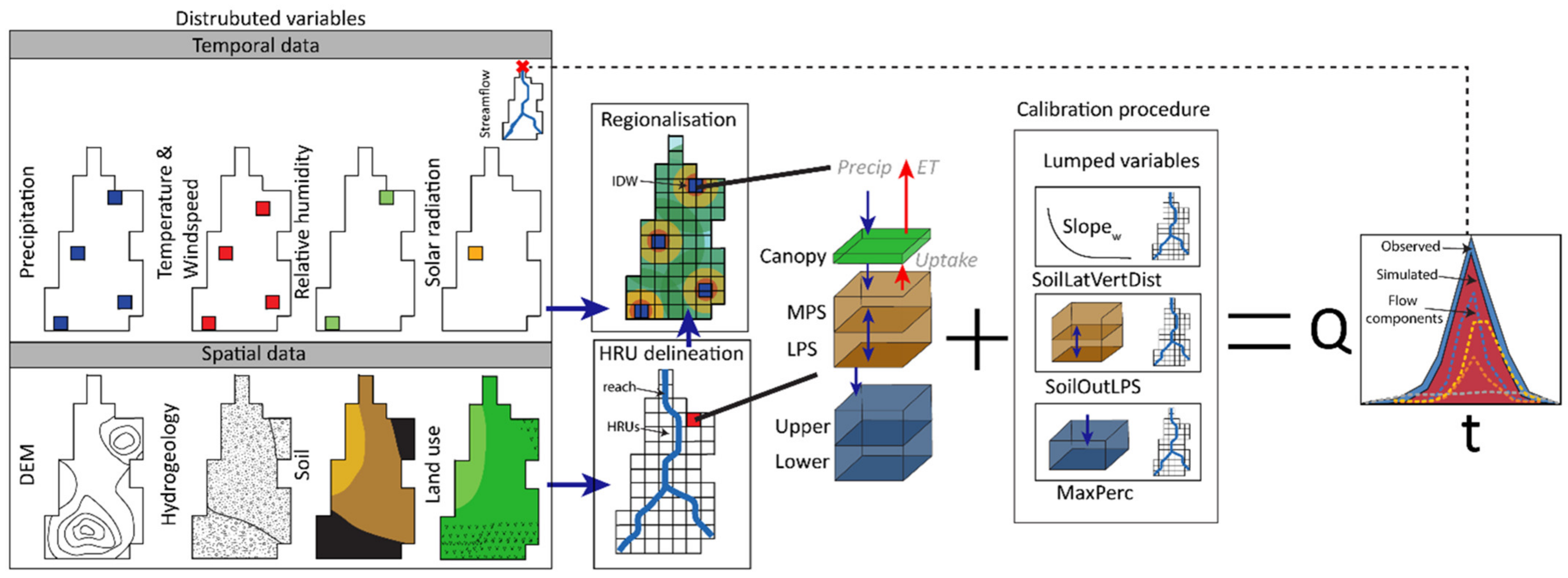
2.2. The JAMS/J2000 Rainfall–Runoff Model

The hydrological conditions of the study catchments (Verlorenvlei, Berg, Eerste, Bot and Breede) were modelled using the fully distributed, process-based JAMS/J2000 rainfall-runoff model [25,39]. The JAMS/J2000 uses two data types, namely spatial and temporal data (Figure 3).
Spatial data, which includes a digital elevation model (DEM) and maps of hydrogeology, soil and land use, form the inputs in a hydrological response unit (HRU) and reach delineation, which are the spatial model constraints [41,42] (Figure 4). Temporal data, which comprise the climate forcings (including all climate variables), were regionalized using inverse distance weighting (IDW) with the spatial position of each of the datasets. IDW is one of the most common interpolation techniques [43], and it performs well for dense precipitation networks [44] and is more suited for discontinuous climate records. Streamflow was likewise temporal data, but was used in the model calibration and validation (except when including reservoir releases; refer to [20]) and was not regionalized. Below, an overview is provided of the climate and streamflow data used for the simulations from 1990 to 2002, as well as the maps of hydrogeology, soil and land use with the model parameters applied to each datatype. Each model’s spatial constraints and the relative size of each HRU (0.4 km2) and sub-basin (7.2 km2) were standardized using the HRU delineation methodology in [18]. The methodology includes a description of the conceptual layout of the simulated hydrological processes and their variables, the subsequent calibration of each model and the sensitivity of the various parameters for each study catchment.

2.2.1. Climate Inputs

Daily totals of precipitation and solar radiation, mean daily relative humidity, temperature, windspeed and maximum and minimum daily temperature were collected for the period 1988–2002 (including a 2-year initialization period). The data were attained from the World Meteorological Organisation (WMO) as global surface summary of the day (GSOD) data [23], as well as the Agricultural Research Council (ARC), the South African Weather Services (SAWS), the Department of Water Affairs and Sanitation, South Africa (DWS), the South African Earth Observation Network [45] and previous JAMS/J2000 model data [18,46,47,48,49,50]. In total, 97 precipitation, 24 temperature, 12 relative humidity, 15 windspeed and seven solar radiation stations were used (Table 2). While the number of available stations varies within each catchment, stations are also shared across catchment boundaries. The average HRU distance to the precipitation stations in each catchment was used to understand the spatial climatic variability across the climate inputs for each catchment (precipitation is regarded as the main climate force for information) (Figure 5). While the climate data provides the hydrological modelling inputs, the data were also analyzed separately according to catchment and mountainous regions in Section 3.1.

2.2.2. Streamflow Gauges

Average daily streamflow (m3 s−1) was collected from the Department of Water Affairs and Sanitation (DWS) for each catchment nearest to the catchment outlet for the period 1990–2002 [19]. Additionally, reservoir outflow data from Kleinplaas (Eerste) and Theewaterskloof (Breede) were collected from the DWS for the modelling period (Berg River dam and Wemmershoek dam outflow only available after 2004). While the catchments, such as Berg (seven reliable stations) [18], Eerste (four stations; two decommissioned after 2000) [19] and Breede (five stations) [51], contain multiple gauges for different sub-basins, the bulk streamflow signature was the only data considered in this approach. In total, the percentage gauged area considered varied between the different catchments, but was between 12 and 79% (Supplementary Materials, Table S1).

2.2.3. Hydrogeology Data

A 1:250,000 geological map of the Western Cape, obtained from the Council of Geosciences (CGS [52,53,54]), formed the input spatial hydrogeological map that was used in the HRU delineation. Hydrogeological properties, including (1) maximum storage capacity (RG1 and RG2max) and (2) storage coefficient (RG1 and RG2_k) for the upper (RG1) and lower aquifer (RG2), were assigned to each spatial hydrogeological unit using regional literature [34,55] and bulk aquifer properties [56,57] (Table 3).

2.2.4. Soil Data

The soil input parameters for the JAMS/J2000 model were determined using the Harmonized World Soil Database (HWSD) (Version 1.2) (30 arc seconds) [58] and the Rosetta lite pedotransfer function within the HYDRUS model [59]. The soil textural characteristics from the HSWD for the top and sub-soil include depth, %sand, silt and clay (SSC) which through a pedotransfer function and a constant upper and lower head boundary are used to generate a soil water retention curve (theta vs. depth). Middle pore storage (MPS: 0.2–50 µm) and large pore storage (LPS: >50 µm), which represent soil water holding capacities at field capacity and the amount of water held against gravity, were determined from three pressure ratings, namely, 0 mbar, 60 mbar and 15,000 mbar, using the derived soil water retention curve. By subtracting the water content between 15,000 mbar and 60 mbar, MPS was determined. LPS was determined by subtracting the water holding capacities between 0 mbar and 60 mbar. The total MPS and LPS volumes are then multiplied by their respective depths and assigned to each of the HSWD soil type values. Finally, two calibration parameters, AC adaption (aircap) and FC (field cap) adaption, were used to scale MPS and LPS, respectively, for each of the study catchments.

2.2.5. Land Use Data

The 2013–2014 South African National Land-Cover dataset [27] was used as the input map, which formed the basis for the land use parameters for the JAMS/J2000. While a landcover map existed in 2000 for the study catchments (and the entire country), the 2013–2014 version includes a more detailed separation of the different management and landcover classes.
The land use model parameters include: (1) albedo (%), (2) monthly surface resistances assuming sufficient water supply, (3) leaf area index (LAI) for vegetational growth periods, (4) effective vegetation heights for growth periods, (5) root depth and (6) sealed grade value (impervious areas). To constrain these respective values for each land use class within the dataset, the literature [60,61,62,63], together with model expertise, was used. While these parameters were mainly used to determine the daily potential evapotranspiration for each HRU, a vegetation interception (a_rain) and linear reduction of potential evapotranspiration according to soil moisture (soilLinRed) were included as model calibration parameters.

2.3. Model Structure and Process Simulation

A simplified water balance equation can be used to describe the process simulation of the JAMS/J2000 model (based on [25,39]) as:
P = Q s + E T + Δ S
where P is the net precipitation, Q s is streamflow, E T is evapotranspiration and Δ S is the change in storage (soil water, groundwater storage, reservoir storage). Furthermore, the separation of streamflow Q s can be written as:
Q s = R D 1 + R D 2 + R G 1 + R G 2
where R D 1 is fast direct runoff and has the highest temporal dynamics and consists of runoff from sealed areas and surface runoff under saturated soil conditions (excluding snow processes), R D 2 is slow direct runoff, which is generated from lateral flow in the soil zone, R G 1 is fast groundwater flow, which is generated conceptually from joint aquifer and loose rock, and is indicative of properties of quaternary sediments, weathered material and fractured rock aquifers and R G 2 is slow groundwater, which relates to regional groundwater flow, including baseflow from shale and basement aquifers. The above-mentioned simplified equations describe the basis for hydrological process simulation and the flow component separation used in this study. The parameters of the JAMS/J2000 model can be grouped into: evapotranspiration, soil water, groundwater and flow routing processes (Table 4). For further descriptions of each of the model parameters and the processes that they were involved in, refer to [25,64].

2.4. Model Calibration and Validation

The model calibration was performed using a semi-automated procedure (e.g., [66]), which utilized the non-dominated sorting genetic algorithm (NSGA-II) [67] to explore the ‘optimal’ parameter space and model expertise from other applications [18,46,48,49,68,69] to finally select quantifiable model parameters for the region. For the calibration and validation of the Velorenvlei, Berg, Bot and Breede catchments, the time series was split into two (e.g., [70]), with (1) calibration from 01-01-1990 to 31-12-1995 and (2) validation from 01-01-1996 to 01-01-2002. As streamflow data for the Eerste catchment (Klein Welmoed-G2H040) was only available post 1995, the model calibration was performed from 01-01-1999 to 31-12-2005. Missing streamflow observations were not considered as part of the calibration and validation for each catchment, and a subsequent validation for Eerste was not possible with the available climate records.
The evaluation of the model’s performance utilized various efficiency criteria that aim to assess different aspects of the simulated hydrograph [71,72,73,74]. The selected efficiency criteria include the Nash–Sutcliffe efficiency (NSE) [65] in standard squared form (E2), logarithmic form (logE2), the relative volume error (pBias) and the Kling-Gupta efficiency (KGE) measure [75]. The NSE criteria used to evaluate each model performance were split into: very good/excellent E > 075; good 0.65 < E ≤ 0.75; satisfactory 0.5 < E ≤ 0.65; unsatisfactory/poor E ≤ 0.5, according to [76]. Visualizations, calculations of the water balance, as well as the relative similarity of each catchment (geology, soil, land use and climate) was used to assess the selected set of model parameters.

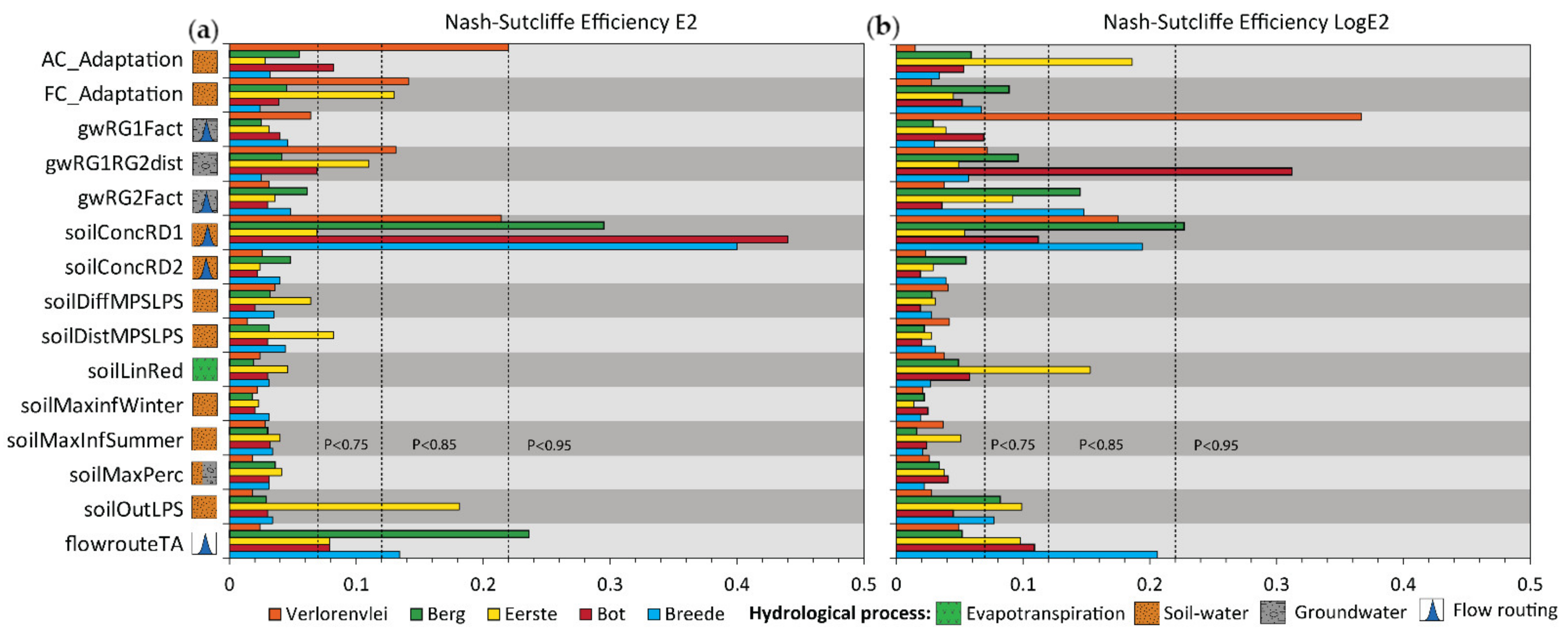
2.5. Sensitivity Analysis

A regional sensitivity analysis (RSA), or what is commonly called a Monte Carlo analysis (MCA) [77], was used to understand the relative importance of the different parameters in the hydrological process simulation of the study catchments using the J2000/JAMS model [78]. In order to understand the relative sensitivities of each of the model parameters, a met model approach was applied whereby a set of scaling factors p was increased/decreased by up to 10% (0.9 p_cal,1.1 p_cal) during the calibration period using the selected optimal parameter value (Table 4). The results from the MCA were used in a simplified regression model to predict the model’s efficiency using a set of scaling factors. The regression model was created using an artificial neural network (ANN), which was trained with the MCA results [79].

3. Results

The results include the analysis of the precipitation amount and characteristics and the resulting observed streamflow (hydrological signatures) of each catchment, as well as the simulated streamflow, simulated hydrological flow components (surface runoff, interflow and baseflow), the simulated water balance and the sensitivity of each parameter for the selected study catchments. While JAMS/J2000 is a daily rainfall–runoff model, monthly outputs were also used to assess the model’s ability to represent seasonal conditions. The simulated results were split into small catchments (Verlorenvlei, Bot and Eerste at <2000 km2) and large catchments (Berg and Breede at >5000 km2).

3.1. Observed Precipitation

For the periods 01-01-1990 to 31-12-1995, Verlorenvlei, Berg, Eerste, Bot and Breede had an average HRU to precipitation station distance of between 10 and 20 km (Figure 5a,b). For the periods 01-01-1996 to 12-31-2002, Berg and Bot maintained relatively the same distance (10–20 km), but for Verlorenvlei, the distance increased to 28 km, while for Eerste, it increased to 50 km and Breede to 28 km. Overall, Bot and Eerste had the highest average yearly precipitation, with between 680 and 790 mm/yr., while Berg and Breede had between 500 and 530 mm/yr. The average yearly precipitation for Verlorenvlei was lowest at 390 mm/yr. The maximum regionalized daily precipitation for Verlorenvlei was 50.4 mm in 1997, while 48.6 mm was received in 1990. For the Berg, Eerste, Bot and Breede, the maximum regionalized daily precipitation was 37.8 mm, 113.5 mm, 99.3 mm and 58 mm in the years 1990, 1993, 1998 and 1993, respectively. Other significant precipitation events for Berg, Eerste, Bot and Breede include 34.8 mm, 48.2 mm, 86 mm and 58 mm in the years 1992, 1991, 1993 and 1998, respectively. On average, Verlorenvlei had 90 precipitation events per year for the period 1990–2002, compared with 117, 137, 140 and 145 events for Berg, Eerste and Breede, respectively. The precipitation data show two dry periods between 1994 and 1995 and 1997–2000 where precipitation was 10% and 20% less, respectively, from the median (Figure 6a). Seasonally, precipitation was mainly received in winter, with 38–49% over the June, July and August (JJA) months for the study catchments (Figure 6b). Breede and Bot had more all-year-round precipitation, with 20% of precipitation received for September, October and November (SON). Berg and Verlorenvlei had the least precipitation in December, January and February (DJF) of the study catchments, with 7–9% of the yearly total.

3.2. Observed Streamflow

The maximum daily streamflow for Verlorenvlei, Eerste and Bot was 8.55 m3/s (although the gauge had a DT of 3657 m3/s), 25.85 m3/s and 61.59 m3/s, respectively, compared with 645.39 m3/s and 1108.14 m3/s for Berg and Breede for the period 01-01-1990 to 31-12-2002 (Figure 7). On average, daily streamflow was 0.35 m3/s, 1.88 m3/s and 0.74 m3/s for Verlorenvlei, Eerste and Bot, respectively, compared with 20.64 m3/s and 37.25 m3/s for Berg and Breede for the same period (Figure 7 and Supplementary Materials, Figure S1). The monthly streamflow hydrograph for Verlorenvlei and Berg was characterized mainly by flows in June, July and August (JJA), which had between 63 and 64% of the total flow between 1990 and 2002 (Figure 7). Eerste, Bot and Breede had more streamflow in September, October and November than Velorenvlei and Berg (26–30%), but monthly streamflow still exceeded 55% of the total during JJA. Streamflow for March, April and May was between 4.5 and 7% for Verlorenvlei, Berg and Eerste, but exceeded 10% for Bot and Breede. The 30th percentile (baseflow component) of the flow duration curve (FDC) for Berg and Breede was 2.70 m3/s and 4.18 m3/s, compared with 0.30 m3/s, 0.10 m3/s and 0 m3/s for Eerste, Bot and Verlorenvlei for the period 1990–2002 (Supplementary Materials, Figure S1). The log FDC curves show three hydrograph groups: (1) Berg and Breede, (2) Eerste and Bot and (3) Verlorenvlei. The Berg and Breede hydrographs were similar for the 30th percentiles, and both were greater, but both deviated between the 10th and 20th percentiles for the period 1990–2002. The Bot and Eerste hydrographs were similar across the different percentiles, only deviating between the 50th and 65th percentiles. For Verlorenvlei, streamflow occurred for the 30th percentile and the curve was dissimilar to the Berg/Breede as well as Eerste/Bot groups. The coefficient of variation (CV) for Berg and Breede was 2.11 and 2.13, while Eerste and Bot had a CV of 78 and 2.44, respectively (Supplementary Materials, Figure S1). Verlorenvlei had the largest CV of 64.33, with 118 days on average of zero flow (ZDF) for the period 1990–2002.

3.3. Simulated Streamflow

For the calibration period, the Berg River model showed the best performance, with a combined peak flow (E2) and low flow (logE2) efficiency of >0.78 and a bias of <0.03 (Figure 7). On average, daily simulated streamflow was 22.37 m3/s, compared with the observed streamflow of 23.13 m3/s. The Breede model performed well during the calibration, especially at representing low flows (logE2) with an efficiency of 0.79, although peak flow was less well simulated, with the E2 at 0.60. On average, the daily simulated streamflow was 37.26 m3/s, compared with an observed streamflow of 41.65 m3/s, with the most noticeable deviations occurring with the monthly hydrograph’s falling limb. The Eerste model performed very well when simulating peak flow during the calibration period (it had a different period to the other catchments: 1999–2006) with an efficiency of 0.81. Low flows were less well simulated, with an efficiency of 0.67. The average daily streamflow simulated for Eerste was 1.71 m3/s, compared with the observed streamflow of 1.77 m3/s, with noticeable deviations in the monthly hydrograph during the months of August to November. The Verlorenvlei and Bot models had a satisfactory (logE2) simulation with an efficiency of >0.54, but peak flows (E2) were poorly simulated, with an efficiency of 0.22 during the calibration period. On average, the daily streamflow simulation for Verlorenvlei was 0.43 m3/s, compared with an observed streamflow of 0.36 m3/s. In contrast, the daily average simulated streamflow for Bot was 1.06 m3/s, compared with an observed streamflow of 0.89 m3/s. For the monthly hydrograph, both models tended to over-simulate streamflow from February to July, with a monthly simulated streamflow of 1.00 m3/s for Bot and 0.62 m3/s for Verlorenvlei, compared to the monthly observed streamflow of 0.78 m3/s and 0.31 m3/s, respectively.
For the validation period, the Berg River model performed similarly, albeit with a slightly lower efficiency of 0.76 for peak flow (E2) and 0.72 for low flow (logE2), which was lower than during the calibration period (Figure 7). The Breede model performed poorly for the simulation of peak flow (E2) during the validation period, with the efficiency dropping to 0.39, although low flow simulations (logE2) were satisfactory, with an efficiency of 0.63. The Bot model performed satisfactorily during the validation, with peak flow efficiency (E2) increasing to 0.52, while low flow (logE2) simulation efficiency remained between 0.65 and 0.68. For Verlorenvlei, the model performed poorly during the calibration and prior to the gauge closure in 2006, where the peak flow (E2) simulation dropped to an efficiency of –0.03, while low flow (logE2) simulation lowered to an efficiency of 0.48. While the validation of Eerste was not possible within the analysis period, the model performed satisfactorily for the period 2006–2012, though less credibly than other models, but with an efficiency of 0.6 for peak flow (E2) and 0.63 for low flow (logE2).

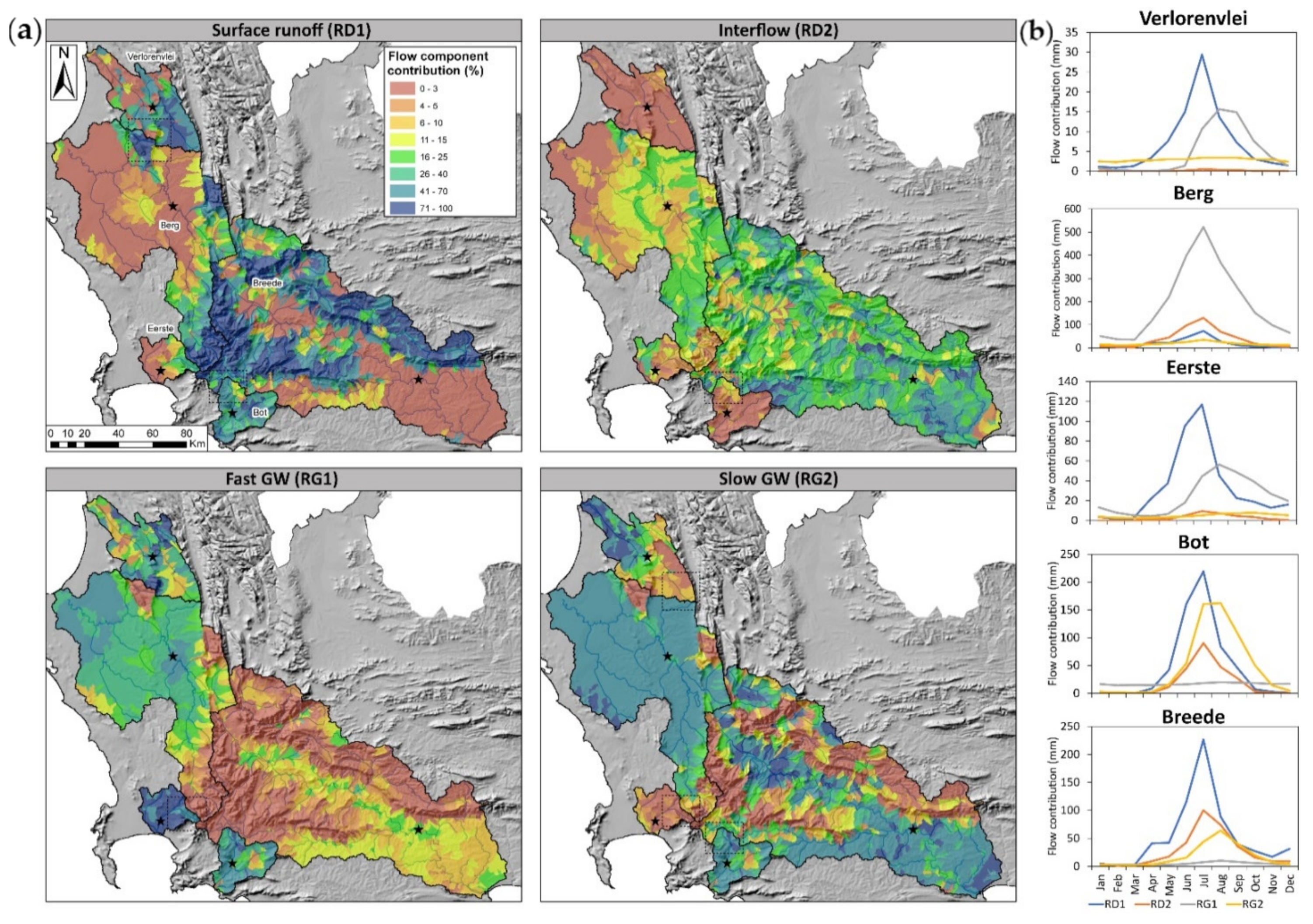
3.4. Simulated Flow Components and Water Balances

The simulated streamflow was made up of the flow components that include RD1 as the surface runoff, RD2 as the interflow, RG1 as the fast groundwater flow and RG2 as the slow groundwater flow (Figure 8). Furthermore, the collective hydrological representation of each model was visualized according to the catchment water balance, which is the simulated streamflow as a percentage of evapotranspiration (Figure 8b), as well as the flow components, which are represented as the combined total streamflow across all the catchments. The optimized parameters (based off the ‘best’ NSGA-II efficiencies) result in Verlorenvlei and Bot having a streamflow composition of less than 10%, with Verlorenvlei having a streamflow composition of less than 5% (Figure 8). The time of concentration (Tc) of the streamflow was 6, 4, 3 and 2 days for Berg, Verlorenvlei, Breede and Bot, respectively, while for Eerste, streamflow reached the outlet in 1 day. Overall, Eerste, Berg and Breede had a streamflow contribution of more than 20%, with as much as 38% streamflow for Eerste (Figure 8).
The results show the general dominance of surface runoff (except for Eerste) in the simulated hydrograph during the wet period (May to July), with between 51 and 36% of the total flow (Figure 9), as well as in the combined total flow with contributions of between 0.28 and 1% (Figure 8). For Eerste, simulated interflow controls the hydrograph during the wet period (May to July), with 55% of the total flow, due to a large sub-surface water storage, while surface runoff was the next most dominant with 22% (Figure 9). The maximum interflow simulated for Berg, Eerste and Breede was 0.08–0.27% of the combined total flow (Figure 8). Simulated fast groundwater flow for Verlorenvlei and Bot control the hydrograph from August to December, with between 31 and 37%, while for Berg, simulated slow groundwater was more dominant, with 36% of the total flow (Figure 9). Simulated slow groundwater (RG2) reached a maximum of 0.27% of the combined total flow for Berg compared with 0.17% for Breede (Figure 8). Verlorenvlei, and in particular the Piketberg mountains, was simulated as 0–0.02% of the combined total flow using the Verlorenvlei model, while the Berg model simulated between 0.18 and 0.27% for the area the within the Berg River catchment (Figure 8). The surface runoff from the headwaters of the Bot was simulated as 0–0.02% of the combined total flow compared with 0.08–0.11%, which falls within the Breede model (Figure 9).

3.5. Model Parameter Sensitivity

The model parameter sensitivity was grouped according to parameters that were not sensitive (percentile < 0.75), moderately sensitive (percentile 0.75–0.85) and highly sensitive (percentile > 0.95) (Figure 10). For the smaller catchments, the scaling factors used to increase/decrease soil water storages (AC_Adaptation and FC_Adaptation) were moderately sensitive, with values of between 0.07 and 0.8 for Bot, Verlorenvlei and Eerste, collectively for the efficiencies E2 and logE2 (Figure 10). Likewise, Berg was sensitive to the scaling of the soil field capacity (FC_Adaptation) during low flow (logE2) simulation, with a value of 0.07. The fast groundwater flow delay parameter (gwRG1Fact) was highly sensitive for Verlorenvlei, with a value of 0.37 (logE2). The distribution parameter for slow and fast groundwater runoff (gwRG1RG2dist) was sensitive for Eerste, Verlorenvlei and Berg, with values of 0.11 (E2), 0.13 (E2) and 0.096 (logE2), respectively. The baseflow delay parameter (gwRG2Fact) was moderately sensitive for Berg and Breede in simulating low flows, with values of 0.145 and 0.148 (logE2), and sensitive for Eerste, with values of 0.092 (logE2). The surface runoff delay parameter (soilConcRD1) was highly sensitive for Berg, Bot and Breede, with values of 0.29, 0.44 and 0.4 (E2). Verlorenvlei showed moderate sensitivity for the soilConcRD1 metric, with a value of 0.2 (E2). The MPS/LPS distribution coefficient for inflow parameter (SoilDistMPSLPS) was sensitive for Eerste, with a value of 0.082 (E2), as well as for the parameter that governed the reduction of potential evapotranspiration according to soil moisture (soilLinRed), with a value of 0.15 (logE2). The outflow parameter of the large pore storage (soilOutLPS) was moderately sensitive for Eerste, with a value of 0.18. The stream routing parameter (overall dampening of the hydrograph) (flowrouteTA) was highly sensitive for Berg, with a value of 0.23 (E2), while for Breede, Eerste and Bot, it was moderately sensitive, with values of 0.13 (E2), 0.08 (E2) and 0.1 (logE2), respectively.

4. Discussion

The broad aim of this study was to develop an understanding of the hydrological variability in mediterranean South Africa using the JAMS/J2000 rainfall–runoff model. The specific objective was to develop a set of model parameter combinations which were able to simulate these regional conditions to better understand runoff generation and storage mechanisms in the WC, but also for further climate change-related assessments. However, a number of factors influence the ability to develop a regional consensus, which can be grouped into: (1) model-related limitations (catchment size, periods of zero flow, parameter equifinality), (2) observed data limitations (streamflow gauge locations, observed rainfall–runoff behavior, low climate station density, anthropogenic impacts) and (3) model input accuracy (soil information, effects of scale) (refer to Section 4.2).

4.1. Hydrological Heterogeneity in WC and Implications for Sustainability

Orographic lifting is an important process that controls precipitation characteristics in mountainous regions around the world, as well as the WC, where elevation and yearly precipitation have a good correlation (R2 = 0.64). As a result, hydrological flows in the WC, and particularly for the Berg and Breede simulation, were dominated by mountainous regions where surface runoff is generated from higher average precipitation (compared to valley regions) and the steep slopes of the TMG (Figure 8). These fractured rock aquifers are likewise an important source of baseflow, with groundwater recharge rates of between 13 and 27% of MAP [80,81], illustrated by the dominance of slow groundwater flow in these models. Interflow, by contrast, occurs in valley regions, but is less significant in the context of the Berg and Breede and is only significant for the Eerste, where sub-surface water storage was more prevalent (Figure 8). The dominance of interflow for the Eerste river was supported by significant bank storage (or transmission loss) which occurs between the upper and lower sub-basins.
Centralized water supply systems, such as the reservoirs used by water management agencies in the Western Cape, rely on streamflow contributions from mountainous regions as source water. The reservoirs that form part of this modelling approach were all located in the winter precipitation regions of the Western Cape, receiving around 38–49% of yearly precipitation over JJA. Concerns over the dominance of centralized water supply systems [82] have recently been borne out by dry periods between 2015 and 2018 in the WC. Recent applications of drought-related indices, such as the soil moisture deficit index (SMDI) [20] and the standardized precipitation index (SPI) [83] suggest that MAM precipitation has been the main period of meteorological shortfalls, with reductions of between 50 and 70%. Although reductions in JJA precipitation were between 20 and 35% for drought periods, shortfalls in MAM had knock-on effects on streamflow generations in JJA and SON. As a result, hydrological flows were mainly generated during these periods with ±60% of the total streamflow, with SON as the next most significant months with as much as 30%. For the remaining 6 months, streamflow, and in particular surface runoff, contributions were limited, due to fewer precipitation events, as well as a high daily evapotranspiration [13]. As a result, reservoirs in the Western Cape are particularly vulnerable to shortfalls in winter precipitation, as well as being subject to considerably high open water evaporation rates during dry summer months.

4.2. Effect of Streamflow Characteristics on Regional Hydrological Modelling

Climate change-related assessments generally utilize regional hydrological models [84] due to the coarse resolution and low pixel variability of Earth system models (ESMs) [85], such as outputs from CORDEX (+−25 kms). As a result, large catchments or a combination of different smaller catchments are more favorable for future climate change-related assessments. However, basic runoff generation mechanisms need to be understood and incorporated for realistic model simulation and assessment.
These impacts were evident in the hydrological model applications for the selected catchments in this study, which have a combined area of 23,500 Km2 (940 pixels for CORDEX outputs). These simulated hydrological processes, which utilize different gauged areal percentages (Supplementary Materials, Figure S2), show similarities for the large catchments, Berg and Breede (Figure 8). Smaller catchments have significantly different hydrological process simulation requirements (Figure 9). While surface runoff and fast groundwater still dominate the simulated hydrographs for Verlorenvlei and Bot, the model still aims to dampen the hydrological response through evapotranspiration, illustrated by a streamflow contribution of <10% (Figure 8b), as well as routing the bulk of water to soil water storage. The Verlorenvlei model, which has a gauge positioned in a sub-basin with a low TMG area (Supplementary Materials, Figure S2 and Table S3), was influenced by the need to simulate days of zero flow, as baseflow contributions from the MG aquifer were limited. These conditions result in the model showing anomalously high sensitivity to the upper groundwater delay (gwRG1Fact) and groundwater distribution (gwRG1RG2dist). The Bot model includes baseflow contributions from the TMG aquifer, but, overall, the gauged area only includes 29% of the catchment (Supplementary Materials, Table S1) and therefore the effective modelling area was small (252 km2). The Bot model likewise showed high sensitivity to groundwater distribution (gwRG1RG2dist). The Eerste model also includes a small effective gauged area (328 km2), but in addition was influenced by wastewater outflows, irrigation and reservoir releases. While reservoir releases were simulated, there were no data available to include the impacts of wastewater outflows and irrigation. As a result, sensitivities in scaling soil water storage (AC and FC adaption) which can be used to compensate for a higher/lower streamflow dynamic, show the impact of anthropogenic factors for Eerste and Berg (Wemmershoek reservoir releases were not included as there were no available outflow data), as well as the effects of the small overall catchment size for Eerste and Bot.
Commonly, sensitivity analyses accompany most current hydrological model applications. However, often it is difficult to identify whether these sensitivities can be caused by anthropogenic factors, whether the noise-to-frequency (water balance) ratio causes anomalously high parameter sensitivity and where distinct streamflow characteristics are responsible for parameter uncertainty. As a result of the observed streamflow characteristics, the effective modelling area and anthropogenic factors, the model parameters selected from the automated calibration for Verlorenvlei, Eerste and Bot were ‘unrealistic’ in a regional context (Figure 8) and impact the uncertainty of previous studies [47,48,49]. While in general the selection of large catchments for regional hydrologically related assessment within a specified region provide lower uncertainty [86], multiple adjacent model applications are still required for catchments affected by anthropogenic factors and regionally unrepresentative streamflow characteristics.

4.3. Uncertainties in Modelling Hydrological Change

Distributed rainfall–runoff models have been used in numerous studies as predictive tools to assess the impact of different climate change projections on future water resource availability around the world [87,88,89]. In South Africa, the most comprehensive assessment includes the analysis of three different global circulation models (GCMs) (CNRM-CM3, ECHAM5/MPI-OM, IPSL-CM4), which, in combination with the A2 emission scenario, projected severe hydrological droughts for much of the Western Cape when comparing present and future conditions (1971–1990 and 2081–2100) [90]. While there have been numerous improvements to GCMs and Earth system models (ESMs), recent studies also aim to use different representative concentration pathways (RCPs) (which replaced emission scenarios), as well as multiple rainfall–runoff model parameter combinations, to constrain future hydrological uncertainties [91]. However, concerns have been raised about the ability of conceptual ‘bucket’ type rainfall–runoff models to simulate multi-year droughts and slow declines in groundwater storage [92], which has reduced model confidence under specific climate change scenarios.
The recent Western Cape drought showed signs of hydrological change (2015–2018), where rainfall–runoff modelling was unable to represent these recent conditions [20]. As groundwater levels showed rather abrupt changes as opposed to multi-year drought trends, and widespread groundwater overuse was postulated, the hydrological change thus far has been associated with hydroclimate shortfall and anthropogenic factors. However, the dynamic of abrupt water use (over days/months) and slow recharge (sometimes over years) still requires further research. A shift in seasonality could impact hydrological simulations and longer, drier summer conditions have already been detected in the region [20]. Furthermore, a shift in precipitation from mainly winter to all-year precipitation would significantly impact water management, water supply systems and natural vegetation, and also future hydrological simulations in the WC, especially seasonally based parameters (SoilMaxInfSummer and SoilMaxInfWinter).
While these impacts and the variations of these parameters have been tested in Bot where parts of the catchment receive all-year precipitation, the structural and component setups of the models require investigation, especially in a larger catchment with lower overall uncertainty. Furthermore, these seasonal changes would likely result in model development, requiring a more detailed breakdown of seasonal parameters, which can then both simulate past, as well as present climate conditions.
As climate change threatens to impact yearly precipitation amounts, climate seasonality and the adaptive strategies used to counteract these impacts, detailed monitoring and measurements are needed to develop sustainable water use practices. Data scarcity in much of Southern Africa limits model application and heightens uncertainty. The lack of high-altitude precipitation stations in the WC impacted the overall simulation of peak flows in this study. Without the improvement of streamflow and precipitation gauging networks in the region, the results of these models cannot be evaluated, nor can they be used to form tools for future flood forecasting. The use of isotopes to validate hydrological process simulation (such as [93]) has the potential to reduce model uncertainties and improve the application of hydrological modelling tools.

4.4. Importance of Sustainable Groundwater Use in the WC

While the introduction of groundwater into the Western Cape water supply network provides a means of improving water security in the region, the use of groundwater by the agricultural sector outside of drought periods could have long-term effects on the sustainability of aquifers in the WC. While improving water security in the context of climate change is important, the long-term sustainability of groundwater is potentially at risk if these aquifers are over utilized. Furthermore, baseflow reductions as a result of groundwater overuse and changes in reservoir releases, as a result of drought, are a major threat facing globally significant wetlands systems, such as Verlorenvlei and Botrivervlei (Ramsar no. 525 and 2291), and this study confirms the importance of regional groundwater flow in the WC. Such effects have already been evident in the recent 2015–2018 drought, where hydrological flow was reduced by as much as 47% during winter [20], as well as in other situations around the world [94]. Knock-on effects follow unsustainable groundwater use, especially affecting groundwater-dependent ecosystems, riparian vegetation and estuarine lakes, which are already pressurized by temperature change and global biodiversity loss.
As the Verlorenvlei is currently under a state of collapse due to prolonged dry conditions [95], other significant wetland systems in the region could also begin to feel the effects of climate change and anthropogenic water use impacts. While numerous studies have endeavored to determine the ecological reserve requirements for many river systems in South Africa (e.g., [96,97]), thereby ensuring more sustainable water use, reservoir releases currently favor agricultural requirements and do not consider the potential changes in the future climate. Similarly, climate change is not considered to be an input in water yield studies and assessments, which only look at human and economic demand. Ensuring detailed hydrogeological assessments and investigations to determine sustainable groundwater abstraction rates, from both large well fields and in the boreholes used by local farmers, is important in reducing streamflow reduction under climate change.

5. Conclusions

Hydrological flows are spatially and temporally complex, and are also dependent on a variety of feedback loops and dependencies within different processes and land features. Understanding hydrological process variability, which is needed for sustainable water management, requires sufficient biophysical, meteorological and hydrological data. Rainfall–runoff models can simulate these different processes and flow component dynamics (surface runoff, interflow and baseflow), but are influenced by catchment size, different anthropogenic factors (irrigation, reservoir release and wastewater outflows), the frequency of the signal-to-noise ratio (water balance) and model-related limitations. A multi-catchment approach provides a means to assess hydrological process variability in a region and determine factors which impact model uncertainty. In mediterranean South Africa, surface runoff was determined as the most significant for hydrological flow, with 44% of the total, followed by baseflow (fast and slow groundwater) with 37%. Large catchments have lower model uncertainties in JAMS/J2000, and the position of relevant gauging instruments was important for reducing model uncertainty and attaining regionally ‘realistic’ simulations. This occurs because the JAMS/J2000 model conceptualizes mesoscale catchments well, but is challenged by microscale catchments where processes are less generalized and data are often not available. Ensuring sustainable groundwater use within the Western Cape is important for reducing streamflow reduction, which is illustrated by the importance of regional groundwater in simulated streamflow. As the occurrence of droughts in many parts of the world is increasing and driving hydrological change, separating climate change-related impacts from anthropogenic factors, such as irrigation and reservoir releases, are important for reducing riverine ecosystem loss and declines in surface water resources.

Supplementary Materials

The following are available online at https://www.mdpi.com/article/10.3390/su132414058/s1, Supplementary Figure S1: (a) Flow duration curve and (b) log flow duration curve of measured streamflow data in each study catchment with statistics of Zero flow days (ZDF), daily average flow (m3/s); Figure S2: Total area of the Table Mountain Group (TMG), Malmesbury Shale (MG), Alluvial sediments and Cape Granite Suite for each catchment and the gauged sub-basin (transparent colours) where the MG shales group include other shales such as the Witteberg, Ecca, Dwyka, Bokkeveld and Uitenhage and the alluvium include quaternary sediments and unclassified units; Table S1: The total gauged area (streamflow) of each of the study catchments with the percentage of the catchment area; Table S2: A list of the parameters and the parameter ranges used in the Monte-Carlo Analysis which was used to generate the sensitivity analysis to understand the relative importance of different parameters for each catchment’s simulated streamflow; Table S3: Total area of the Table Mountain Group (TMG), Malmesbury Shale (MG), Alluvial sedi-ments and Cape Granite Suite for each catchment and the gauged sub-basin (transparent colours) where the MG shales group include other shales such as the Witteberg, Ecca, Dwyka, Bokkeveld and Uitenhage and the alluvium include quaternary sediments and unclassified units.

Author Contributions

Conceptualization, A.W., G.M., A.K. and J.H.; Data curation, A.W., A.K., S.K. and J.H.; Investigation, A.K. and J.H.; Methodology, A.W., A.K. and S.K.; Project administration, G.M., S.K. and J.H.; Resources, J.H.; Software, A.W., A.K. and S.K.; Validation, A.W., S.K. and J.H.; Visualization, A.W., G.M., A.K. and J.H.; Writing—original draft, A.W., A.K., S.K. and J.H.; Writing—review & editing, A.W. All authors have read and agreed to the published version of the manuscript.

Funding

The authors would like to thank DAAD (German Academic Exchange Service: sponsored by BMBF (The Federal Ministry of Education and Research)), the Division for Research Development (DRD) of Stellenbosch University and the Department of Water Affairs and Sanitation (DWS) for funding support. The publisher is fully responsible for the content.

Institutional Review Board Statement

Not applicable.

Informed Consent Statement

Not applicable.

Data Availability Statement

The data can be made available on request from the corresponding author.

Acknowledgments

The authors would like to thank the South Africa Earth Observation Network (SAEON), Department of Water Affairs and Sanitation (DWS), South Africa Weather Service (SAWS) and Agricultural Research Council (ARC) and Southern African Science Service Centre for Climate Change and Adaptive Land Management (SASSCAL) for access to climate and streamflow records. The authors would like to acknowledge the contributions of two anonymous reviewers and Jodie Miller for improving the quality of this paper.

Conflicts of Interest

The authors declare no conflict of interest.

References

  1. IPCC. Climate Change 2021: The Physical Science Basis; Contribution of Working Group I to the Sixth Assessment Report of the Intergovernmental Panel on Climate Change; Masson-Delmotte, V., Zhai, P., Pirani, A., Connors, S.L., Péan, C., Berger, S., Caud, N., Chen, Y., Eds.; Cambridge University Press: Cambridge, UK, 2021; in press. [Google Scholar]
  2. Döll, P.; Fiedler, K.; Zhang, J. Global-scale analysis of river flow alterations due to water withdrawals and reservoirs. Hydrol. Earth Syst. Sci. 2009, 13, 2413–2432. [Google Scholar] [CrossRef] [Green Version]
  3. Arnell, N.W.; Gosling, S.N. The impacts of climate change on river flow regimes at the global scale. J. Hydrol. 2013, 486, 351–364. [Google Scholar] [CrossRef]
  4. Beven, K. Interflow. In Unsaturated Flow in Hydrologic Modeling; Springer: Berlin/Heidelberg, Germany, 1989; pp. 191–219. [Google Scholar]
  5. Hall, F.R. Base-flow recessions—A review. Water Resour. Res. 1968, 4, 973–983. [Google Scholar] [CrossRef]
  6. Zeiringer, B.; Seliger, C.; Greimel, F.; Schmutz, S. River Hydrology, Flow Alteration, and Environmental Flow. In Riverine Ecosystem Management: Science for Governing Towards a Sustainable Future; Schmutz, S., Sendzimir, J., Eds.; Springer International Publishing: Cham, Switzerland, 2018; pp. 67–89. ISBN 978-3-319-73250-3. [Google Scholar]
  7. Haddeland, I.; Lettenmaier, D.P.; Skaugen, T. Effects of irrigation on the water and energy balances of the Colorado and Mekong river basins. J. Hydrol. 2006, 324, 210–223. [Google Scholar] [CrossRef]
  8. Marston, R.A. Geomorphology and vegetation on hillslopes: Interactions, dependencies, and feedback loops. Geomorphology 2010, 116, 206–217. [Google Scholar] [CrossRef]
  9. Markovich, K.H.; Manning, A.H.; Condon, L.E.; McIntosh, J.C. Mountain-block recharge: A review of current understanding. Water Resour. Res. 2019, 55, 8278–8304. [Google Scholar] [CrossRef] [Green Version]
  10. Wilson, J.L.; Guan, H. Mountain-Block Hydrology and Mountain-Front Recharge; Wiley: Hoboken, NJ, USA, 2004; Volume 9. [Google Scholar]
  11. Mokua, R.A.; Glenday, J.; Nel, J.; Butler, M. Combined use of stable isotopes and hydrochemical characteristics to determine streamflow sources in the Jonkershoek catchment, South Africa. Isot. Environ. Health Stud. 2020, 56, 238–259. [Google Scholar] [CrossRef] [PubMed]
  12. Tetzlaff, D.; Soulsby, C. Sources of baseflow in larger catchments—Using tracers to develop a holistic understanding of runoff generation. J. Hydrol. 2008, 359, 287–302. [Google Scholar] [CrossRef]
  13. Benito, G.; Thorndycraft, V.R.; Rico, M.T.; Sánchez-Moya, Y.; Sopeña, A.; Botero, B.A.; Machado, M.J.; Davis, M.; Pérez-González, A. Hydrological response of a dryland ephemeral river to southern African climatic variability during the last millennium. Quat. Res. 2011, 75, 471–482. [Google Scholar] [CrossRef] [Green Version]
  14. Flugel, W.A. Hierarchically structured hydrological process studies to regionalize interflow in a loess covered catchment near Heidelberg, Germany. Exchange Processes at the Land Surface for a Range Space and Time Scales. In Proceedings of the International Symposium, Yokohama, Japan, 20–23 July 1993; pp. 215–223. [Google Scholar]
  15. Lange, J. Dynamics of transmission losses in a large arid stream channel. J. Hydrol. 2005, 306, 112–126. [Google Scholar] [CrossRef]
  16. De Clercq, W.P.; Jovanovic, N.; Fey, M.V. Land Use Impacts on Salinity in Berg River Water: Research on Berg River Water Management; Water Research Commission: Gezina, South Africa, 2010; ISBN 9781770059719. [Google Scholar]
  17. Ujeneza, E.L.; Abiodun, B.J. Drought regimes in Southern Africa and how well GCMs simulate them. Clim. Dyn. 2015, 44, 1595–1609. [Google Scholar] [CrossRef]
  18. Watson, A.; Kralisch, S.; Künne, A.; Fink, M.; Miller, J. Impact of precipitation data density and duration on simulated flow dynamics and implications for ecohydrological modelling in semi-arid catchments in Southern Africa. J. Hydrol. 2020, 590, 125280. [Google Scholar] [CrossRef]
  19. DWS Department of Water and Sanitation. 2018. Available online: http://www.dwa.gov.za/Hydrology/Weekly/Province.aspx (accessed on 15 November 2021).
  20. Watson, A.; Miller, J.; Künne, A.; Kralisch, S. Using soil-moisture drought indices to evaluate key indicators of agricultural drought in semi-arid Mediterranean Southern Africa. Sci. Total Environ. 2021. [Google Scholar] [CrossRef]
  21. Zander, F.; Kralisch, S. River basin information system: Open environmental data management for research and decision making. ISPRS Int. J. Geo-Inf. 2016, 5, 123. [Google Scholar] [CrossRef]
  22. Helmschrot, J.; Thompson, S.; Kralisch, S.; Zander, F. The SASSCAL Data and Information Portal. Biodivers. Ecol. 2018, 6, 112–113. [Google Scholar] [CrossRef]
  23. NOA. Global Surface Summary of Day (GSOD); National Centers for Environmental Information: Asheville, NC, USA, 2016.
  24. Arnold, J.G.; Srinivasan, R.; Muttiah, R.S.; Williams, J.R. Large area hydrologic modeling and assessment part I: Model development 1. JAWRA J. Am. Water Resour. Assoc. 1998, 34, 73–89. [Google Scholar] [CrossRef]
  25. Krause, P. Das hydrologische Modellsystem J2000. Beschreibung und Anwendung in großen Flussgebieten. In Umwelt/Environment; Research Centre: Jülich, Germany, 2001; Volume 29. [Google Scholar]
  26. Schulze, R.E.; Maharaj, M.; Warburton, M.L.; Gers, C.J.; Horan, M.J.C.; Kunz, R.P.; Clark, D.J. South African Atlas of Climatology and Agrohydrology: WRC Report 1489/1/06; Water Research Commission: Pretoria, South Africa, 2007. [Google Scholar]
  27. GeoTerraImage. Carbon Sinks Atlas for South Africa; GTI 2013-14 SA Landcover Report; GeoTerraImage: Pretoria, South Africa, 2015. [Google Scholar]
  28. Van Niekerk, A.; Jarmain, C.; Goudriaan, R.; Muller, S.; Ferrerira, F.; Münch, Z.; Pauw, T.; Stephenson, G.; Gibson, L. An Earth Observation Approach Towards Mapping Irrigated Areas and Quantifying Water Use By Irrigated Crops in South Africa; Report No. TT 745/17; Water Research Commission: Pretoria, South Africa, 2018; ISBN 9781431209644. [Google Scholar]
  29. Roffe, S.J.; Fitchett, J.M.; Curtis, C.J. Classifying and mapping rainfall seasonality in South Africa: A review. S. Afr. Geogr. J. 2019, 101, 158–174. [Google Scholar] [CrossRef]
  30. Lynch, S. Development of a Raster Database of Annula, Monthly and Daily Rainfall for Southern Africa; WRC Report No. 1156/1/04; Water Research Commission: Pietermaritzburg, South Africa, 2004. [Google Scholar]
  31. Sinclair, S.A.; Lane, S.B.; Grindley, J.R. Estuaries of the Cape: Part II: Synopses of avaiable information on individual systems. In National Research Institue for Oceanology; Heydorn, A.E.F., Morant, P.D., Eds.; Printing & Publishing Co. (Pty): Cape Town, South Africa, 1986. [Google Scholar]
  32. Johnson, M.R.; Anhauesser, C.R.; Thomas, R.J. The Geology of South Africa; Geological Society of South Africa: Johannesburg, South Africa, 2006. [Google Scholar]
  33. Rozendaal, A.; Scheepers, R. Magmatic and related mineral deposits of the Pan-African Saldania belt in the Western Cape Province, South Africa. J. Afr. Earth Sci. 1995, 21, 107–126. [Google Scholar] [CrossRef]
  34. Conrad, J.; Nel, J.; Wentzel, J. The challenges and implications of assessing groundwater recharge: A case study-northern Sandveld, Western Cape, South Africa. Water SA 2004, 30, 75–81. [Google Scholar] [CrossRef] [Green Version]
  35. Goldblatt, P.; Manning, J.C. Plant diversity of the Cape region of southern Africa. Ann. Mo. Bot. Gard. 2002, 89, 281–302. [Google Scholar] [CrossRef]
  36. Midgley, G.F.; Hannah, L.; Millar, D.; Thuiller, W.; Booth, A. Developing regional and species-level assessments of climate change impacts on biodiversity in the Cape Floristic Region. Biol. Conserv. 2003, 112, 87–97. [Google Scholar] [CrossRef]
  37. Olivier, G.; Helmschrot, J.; de Clercq, W.P. Are large classical gully systems inactive remnants of the past? A field-based case study investigating sediment movement. Biodivers. Ecol. 2018, 6, 146–154. [Google Scholar] [CrossRef]
  38. De Clercq, W.; Jovanovic, N.; Bugan, R.; Mashimbye, E.; Toit, T.; Van Niekerk, A.; Ellis, F.; Wasserfall, N.; Botha, P.; Steudels, T.; et al. Management of Human-Induced Salinisation in the Berg River Catchment and Development of Criteria for Regulating Agricultural Land Use in Terms of Salt Generating Capacity; Research Report: 1849/1/13; Water Research Commission: Pretoria, South Africa, 2013; ISBN 9781431204021. [Google Scholar]
  39. Kralisch, S.; Krause, P.; Fink, M.; Fischer, C.; Flügel, W.A. Component based environmental modelling using the JAMS framework. In Proceedings of the MODSIM07—Land, Water Enviromental Management: Integrated System for Sustainability, Christchurch, New Zealand, 10–13 December 2007; pp. 812–818. [Google Scholar]
  40. Krause, P. Quantifying the impact of land use changes on the water balance of large catchments using the J2000 model. Phys. Chem. Earth Parts A/B/C 2002, 27, 663–673. [Google Scholar] [CrossRef]
  41. Flügel, W.-A. Delineating hydrological response units by geographical information system analyses for regional hydrological modelling using PRMS/MMS in the drainage basin of the River Bröl, Germany. Hydrol. Process. 1995, 9, 423–436. [Google Scholar] [CrossRef]
  42. Pfennig, B.; Kipka, H.; Fink, M.; Wolf, M.; Krause, P.; Flügel, W.-A. Development of an extended routing scheme in reference to consideration of multi-dimensional flow relations between hydrological model entities. In Proceedings of the 18th World IMACS/MODSIM Congress, Cairns, Australia, 13–17 July 2009; pp. 37–43. [Google Scholar]
  43. Ly, S.; Charles, C.; Degré, A. Different methods for spatial interpolation of rainfall data for operational hydrology and hydrological modeling at watershed scale: A review. Biotechnol. Agron. Soc. Environ. 2013, 17, 392–406. [Google Scholar]
  44. Dirks, K.; Hay, J.; Stow, C.; Harris, D. High-resolution studies of rainfall on Norfolk Island. Part IV: Observations of fractional time raining. J. Hydrol. 1998, 208, 187–193. [Google Scholar] [CrossRef]
  45. Slingsby, J.A.; de Buys, A.; Simmers, A.D.A.; Prinsloo, E.; Forsyth, G.G.; Glenday, J.; Allsopp, N. Jonkershoek: Africa’s oldest catchment experiment-80 years and counting. Hydrol. Process. 2021, 35, e14101. [Google Scholar] [CrossRef]
  46. Bugan, R.D.H. Modeling and Regulating Hydrosalinity Dynamics in the Sandspruit River Catchment (Western Cape). Ph.D. Thesis, Stellenbosch University, Stellenbosch, South Africa, 2014. [Google Scholar]
  47. Miller, J.; Watson, A.P.; Fleischer, M.; Eilers, A.; Sigidi, N.T.; Van Gend, J.; Van Rooyen, J.D.; Clarke, C.E.; de Clercq, W. Groundwater quality, quantity, and recharge estimation on the West Coast of South Africa. In Biodiversity & Ecology; Revermann, R., Krewenka, K., Schmiedel, U., Olwoch, J., Helmschrot, J., Jürgens, N., Eds.; Klaus Hess Publishers: Göttingen, Germany; Windhoek, Namibia, 2018; Volume 6, pp. 86–96. ISBN 9783933117953. [Google Scholar]
  48. Watson, A.; Miller, J.; Fleischer, M.; de Clercq, W. Estimation of groundwater recharge via percolation outputs from a rainfall/runoff model for the Verlorenvlei estuarine system, west coast, South Africa. J. Hydrol. 2018, 558, 238–254. [Google Scholar] [CrossRef] [Green Version]
  49. Watson, A.; Miller, J.; Fink, M.; Kralisch, S.; Fleischer, M.; De Clercq, W. Distributive rainfall-runoff modelling to understand runoff-to-baseflow proportioning and its impact on the determination of reserve requirements of the Verlorenvlei estuarine lake, west coast, South Africa. Hydrol. Earth Syst. Sci. 2019, 23, 2679–2697. [Google Scholar] [CrossRef] [Green Version]
  50. Watson, A.P.; Kralisch, S.; Van Rooyen, J.D.; Miller, J. Quantifying and understanding the source of recharge for alluvial systems in arid environments through the development of a seepage model. J. Hydrol. 2021, 601, 126650. [Google Scholar] [CrossRef]
  51. Bangira, T.; Maathuis, B.H.P.; Dube, T.; Gara, T.W. Investigating flash floods potential areas using ASCAT and TRMM satellites in the Western Cape Province, South Africa. Geocarto Int. 2015, 30, 737–754. [Google Scholar] [CrossRef]
  52. Gresse, P.G. Geological Map 3319 Worcester 1:250,000 Scale; Council for Geosciences: Pretoria, South Africa, 1997. [Google Scholar]
  53. Theron, J.N. Geological Map 3318 Cape Town 1:250,000 Scale; Council for Geosciences: Pretoria, South Africa, 1990. [Google Scholar]
  54. Visser, H.; Theron, J.N. Geological Map 3218 Clanwilliam 1:250,000 Scale; Government Printer: Pretoria, South Africa, 1973.
  55. Greenmined Environmental Unit MO1. SRK Preliminary Assessment of Impact of the Proposed Riviera Tungsten Mine on Groundwater Resources Preliminary Assessment of Impact of the Proposed Riviera Tungsten Mine on Groundwater Resources; SRK Consulting: Rondebosch, South Africa, 2009. [Google Scholar]
  56. Domenico, P.A.; Schwartz, F.W. Physical and Chemical Hydrogeology—Hydraulic Testing: Models, Methods, and Applications 1990; Wiley: New York, NY, USA, 1998. [Google Scholar]
  57. Tankard, A.J.; Martin, M.; Eriksson, K.A.; Hobday, D.K.; Hunter, D.R.; Minter, W.E.L. Crustal Evolution of Southern Africa: 3.8 Billion Years of Earth History; Springer Science & Business Media: Berlin/Heidelberg, Germany, 2012; ISBN 1461381479. [Google Scholar]
  58. Batjes, N.; Dijkshoorn, K.; Van Engelen, V.; Fischer, G.; Jones, A.; Montanarella, L.; Petri, M.; Prieler, S.; Teixeira, E.; Wiberg, D. Harmonized World Soil Database (Version 1.2); Technical Report; FAO: Rome, Italy; IIASA: Laxenburg, Austria, 2012. [Google Scholar]
  59. Šimůnek, J.; van Genuchten, M.T.; Sejna, M. The HYDRUS Software Package for Simulating the Two- and Three-Dimensional Movement of Water, Heat, and Multiple Solutes in Variably-Saturated Porous Media; Technical Manual Version 1.0; PC Progress: Prague, Czech Republic, 2006; p. 230. [Google Scholar]
  60. Amer, K.H.; Hatfield, J.L. Canopy resistance as affected by soil and meteorological factors in potato. Agron. J. 2004, 96, 978–985. [Google Scholar] [CrossRef] [Green Version]
  61. Crain, J. Modelling Evaporation from Plant Canopies; Insititue of Hydrology: Oxfordshire, UK, 1998. [Google Scholar]
  62. Johnson, P.A. Variations in Albedo among Natural and Disturbed South Western Cape Veld Types. Master’s Thesis, University of Cape Town, Cape Town, South Africa, 1983. [Google Scholar]
  63. Munitz, S.; Netzer, Y.; Schwartz, A. Sustained and regulated deficit irrigation of field-grown Merlot grapevines. Aust. J. Grape Wine Res. 2017, 23, 87–94. [Google Scholar] [CrossRef]
  64. Kralisch, S.; Krause, P. JAMS—A framework for natural resource model development and application. In Proceedings of the Proceedings of the {iEMSs} Third Biannual Meeting, International Environmental Modelling and Software Society, Burlington, VT, USA, 9–12 July 2006; Voinov, A., Jakeman, A., Rizzoli, A.E., Eds.; pp. 6–11. [Google Scholar]
  65. Nash, J.E. River flow forecasting through conceptual models, I: A discussion of principles. J. Hydrol. 1970, 10, 398–409. [Google Scholar] [CrossRef]
  66. Boyle, D.P.; Gupta, H.V.; Sorooshian, S. Toward improved calibration of hydrologic models: Combining the strengths of manual and automatic methods. Water Resour. Res. 2000, 36, 3663–3674. [Google Scholar] [CrossRef]
  67. Deb, K.; Pratap, A.; Agarwal, S.; Meyarivan, T. A fast and elitist multiobjective genetic algorithm: NSGA-II. IEEE Trans. Evol. Comput. 2002, 6, 182–197. [Google Scholar] [CrossRef] [Green Version]
  68. Rooyen, J.D.; Watson, A.P.; Palcsu, L.; Miller, J.A. Constraining the Spatial Distribution of Tritium in Groundwater across South Africa. Water Resour. Res. 2021, 57. [Google Scholar] [CrossRef]
  69. Treumer, L. Bachelor Thesis Application of MODIS Global Terrestrial Evapotranspiration Data for hydrological modelling in the Western Cape Region, South Africa. Bachelor’s Thesis, Friedrich-Schiller-University, Jena, Germany, 2016. [Google Scholar]
  70. Guo, D.; Zheng, F.; Gupta, H.; Maier, H.R. On the Robustness of Conceptual Rainfall-Runoff Models to Calibration and Evaluation Data Set Splits Selection: A Large Sample Investigation. Water Resour. Res. 2020, 56, e2019WR026752. [Google Scholar] [CrossRef]
  71. Krause, P.; Boyle, D.P.; Bäse, F. Comparison of different efficiency criteria for hydrological model assessment. Adv. Geosci. 2005, 5, 89–97. [Google Scholar] [CrossRef] [Green Version]
  72. Kundzewicz, Z.W.; Krysanova, V.; Benestad, R.E.; Hov, Ø.; Piniewski, M.; Otto, I.M. Uncertainty in climate change impacts on water resources. Environ. Sci. Policy 2018, 79, 1–8. [Google Scholar] [CrossRef]
  73. Legates, D.R.; McCabe, G.J. Evaluating the use of “goodness-of-fit” Measures in hydrologic and hydroclimatic model validation. Water Resour. Res. 1999, 35, 233–241. [Google Scholar] [CrossRef]
  74. Moriasi, D.N.; Arnold, J.G.; Van Liew, M.W.; Bingner, R.L.; Harmel, R.D.; Veith, T.L. Model Evaluation Guidelines for Systematic Quantification of Accuracy in Watershed Simulations. Trans. ASABE 2007, 50, 885–900. [Google Scholar] [CrossRef]
  75. Gupta, H.V.; Sorooshian, S.; Yapo, P.O. Toward improved calibration of hydrologic models: Multiple and noncommensurable measures of information. Water Resour. Res. 1998, 34, 751–763. [Google Scholar] [CrossRef]
  76. Waters, D. Modelling Reductions of Pollutant Loads Due to Improved Management Practices in the Great Barrier Reef Catchments; Whole of GBR, Technical Report; Australian Government: Canberra, Australia, 2014; Volume 1, pp. 1–120.
  77. Hornberger, G.M.; Spear, R.C. Approach to the preliminary analysis of environmental systems. J. Environ. Manag. 1981, 12, 7–18. [Google Scholar]
  78. Kralisch, S.; Fischer, C. Model Representation, Parameter Calibration and Parallel Computing—The JAMS Approach. Available online: https://www.researchgate.net/publication/234081091_Model_representation_parameter_calibration_and_parallel_computing_-_the_JAMS_approach (accessed on 15 November 2021).
  79. Fischer, C.; Kralisch, S.; Krause, P.; Flügel, W.A. An Integrated, Fast and Easily Useable Software Toolbox Allowing Comparative and Complementary Application of Various Parameter Sensitivity Analysis Methods. Available online: https://www.researchgate.net/publication/234081121_An_integrated_fast_and_easily_useable_software_toolbox_which_allows_comparative_and_complementary_application_of_various_parameter_sensitivity_analysis_methods (accessed on 15 November 2021).
  80. Miller, J.A.; Dunford, A.J.; Swana, K.A.; Palcsu, L.; Butler, M.; Clarke, C.E. Stable isotope and noble gas constraints on the source and residence time of spring water from the Table Mountain Group Aquifer, Paarl, South Africa and implications for large scale abstraction. J. Hydrol. 2017, 551, 100–115. [Google Scholar] [CrossRef]
  81. Wu, Y. Groundwater Recharge Estimation in Table Mountain Group Aquifer Systems with a Case Study of Kammanassie Area. Ph.D. Thesis, University of the Western Cape, Cape Town, South Africa, 2005. [Google Scholar]
  82. Sapkota, M.; Arora, M.; Malano, H.; Moglia, M.; Sharma, A.; George, B.; Pamminger, F. An integrated framework for assessment of hybrid water supply systems. Water 2016, 8, 4. [Google Scholar] [CrossRef] [Green Version]
  83. Archer, E.; Landman, W.; Malherbe, J.; Tadross, M.; Pretorius, S. South Africa’s winter rainfall region drought: A region in transition? Clim. Risk Manag. 2019, 25, 100188. [Google Scholar] [CrossRef]
  84. Arnell, N.W.; Hudson, D.A.; Jones, R.G. Climate change scenarios from a regional climate model: Estimating change in runoff in southern Africa. J. Geophys. Res. Atmos. 2003, 108. [Google Scholar] [CrossRef]
  85. Fatichi, S.; Or, D.; Walko, R.; Vereecken, H.; Young, M.H.; Ghezzehei, T.A.; Hengl, T.; Kollet, S.; Agam, N.; Avissar, R. Soil structure is an important omission in Earth System Models. Nat. Commun. 2020, 11, 522. [Google Scholar] [CrossRef] [Green Version]
  86. Xue, Z.; Charonko, J.J.; Vlachos, P.P. Signal-to-noise ratio, error and uncertainty of PIV measurement. In Proceedings of the PIV13; 10th International Symposium on Particle Image Velocimetry, Delft, The Netherlands, 1–3 July 2013. [Google Scholar]
  87. Kim, J.; Habimana, J.D.D.; Kim, S. Assessment of Climate Change Impacts on the Hydroclimatic Response in Burundi Based on CMIP6 ESMs. Sustainability 2021, 13, 12037. [Google Scholar] [CrossRef]
  88. Narsimlu, B.; Gosain, A.K.; Chahar, B.R. Assessment of future climate change impacts on water resources of Upper Sind River Basin, India using SWAT model. Water Resour. Manag. 2013, 27, 3647–3662. [Google Scholar] [CrossRef]
  89. Bhatta, B.; Shrestha, S.; Shrestha, P.K.; Talchabhadel, R. Evaluation and application of a SWAT model to assess the climate change impact on the hydrology of the Himalayan River Basin. Catena 2019, 181, 104082. [Google Scholar] [CrossRef]
  90. Schulze, R.E. A 2011 Perspective on Climate Change And The South African Water Sector; WRC Report No. TT 518/12; Water Research Commission: Pretoria, South Africa, 2012; ISBN 9781431202706. [Google Scholar]
  91. Her, Y.; Yoo, S.H.; Cho, J.; Hwang, S.; Jeong, J.; Seong, C. Uncertainty in hydrological analysis of climate change: Multi-parameter vs. multi-GCM ensemble predictions. Sci. Rep. 2019, 9, 4974. [Google Scholar] [CrossRef] [Green Version]
  92. Fowler, K.; Knoben, W.; Peel, M.; Peterson, T.; Ryu, D.; Saft, M.; Seo, K.W.; Western, A. Many Commonly Used Rainfall-Runoff Models Lack Long, Slow Dynamics: Implications for Runoff Projections. Water Resour. Res. 2020, 56, e2019WR025286. [Google Scholar] [CrossRef]
  93. Stadnyk, T.A.; Delavau, C.; Kouwen, N.; Edwards, T.W.D. Towards hydrological model calibration and validation: Simulation of stable water isotopes using the isoWATFLOOD model. Hydrol. Process. 2013, 27, 3791–3810. [Google Scholar] [CrossRef]
  94. Cooper, D.J.; Wolf, E.C.; Ronayne, M.J.; Roche, J.W. Effects of groundwater pumping on the sustainability of a mountain wetland complex, Yosemite National Park, California. J. Hydrol. Reg. Stud. 2015, 3, 87–105. [Google Scholar] [CrossRef] [Green Version]
  95. Daily Maverick West Coast’s Verlorenvlei: What’s Lost When a Wetland Dries up? 2021. Available online: https://www.dailymaverick.co.za/article/2021-03-13-west-coasts-verlorenvlei-whats-lost-when-a-wetland-dries-up/ (accessed on 15 November 2021).
  96. Hughes, D.A.; Hannart, P. A desktop model used to provide an initial estimate of the ecological instream flow requirements of rivers in South Africa. J. Hydrol. 2003, 270, 167–181. [Google Scholar] [CrossRef]
  97. Van Wyk, E.; Sherwill, T. The Ecological Reserve: Towards a common understanding for river management in South Africa. Water SA 2006, 32, 403–409. [Google Scholar] [CrossRef] [Green Version]
Figure 1. (a) Location of South Africa within Africa; (b) Verlorenvlei, Berg River, Eerste, Bot and Breede study catchments within the Western Cape province, showing the locations of precipitation stations, bulk streamflow monitoring, major reservoirs, major towns and cities within the region.
Sustainability 13 14058 g001
Figure 2. Mean annual precipitation (MAP) for Verlorenvlei, Berg River, Eerste, Bot and Breede catchments within the Western Cape province, where MAP is greater than 1000 mm/yr. in the mountainous regions, reducing to less than 500 mm/yr. in the catchment valleys towards the catchment outlets (based on [30]).
Sustainability 13 14058 g002
Figure 3. Model schematic of the process-oriented JAMS/J2000 ecohydrological model (based on [40]), illustrating the different flow components simulation, the model modules used as part of the simulation as well as the different calibration factors (based on [25]).
Sustainability 13 14058 g003
Figure 4. A schematic of the modelling procedure used by the JAMS/J2000 model (based on [25]), including the spatial data, which were used in the HRU delineation, and the temporal data, which were regionalized using IDW. This is a simplified view of the simulated processes of each HRU together with the calibrated parameters, which were used to simulate the catchment’s hydrological flow components (surface runoff, interflow and baseflow) and combined (streamflow) to evaluate the model performance.
Sustainability 13 14058 g004
Figure 5. (a) Temporal and (b) spatial aggregate of the average distance between the precipitation stations and the delineated HRUs for the period 1990–2002. Berg and Eerste had a high station distance (0–5 km) in the catchment headwaters, while Verlorenvlei and Bot had a low distance (>20 km). The Breede catchment had relatively high station distance in headwaters (5–20 km) but reduced significantly towards the outlet (>40 km) and for the periods 1998–2002.
Sustainability 13 14058 g005
Figure 6. (a) Regionalized precipitation (IDW) for each of the study catchments for the period 1990–2002. The results show two dry periods between 1994 and 1995 and 1997–2000. (b) Monthly precipitation for the study catchments illustrating the bulk of precipitation during JJA (June, July and August).
Sustainability 13 14058 g006
Figure 7. Simulated (red line), observed streamflow (blue line) and regionalized precipitation (gray bar) split into small catchments (Verlorenvlei, Bot and Eerste at <2000 km2) and large catchments (Berg and Breede at >5000 km2). Simulated and observed streamflow as a monthly average for the calibration period (01-01-1990 to 31-12-1995) and the Nash–Sutcliffe efficiency (NSE, [65]) in standard form (E2), logarithmic form (logE2), relative volume error (pBias) and Kling–Gupta efficiency (KGE) (Gupta et al., 2009) used as model performance criteria for model calibration and validation (01-01-1996 to 31-12-2002).
Sustainability 13 14058 g007
Figure 8. (a) Aggregated simulated surface runoff (RD1), interflow (RD2), fast (RG1) and slow (RG2) groundwater flow for the study catchments, represented as the average amount per year (mm/yr.). (b) Simulated water balance of each catchment (total precipitation, evapotranspiration and streamflow).
Sustainability 13 14058 g008
Figure 9. (a) The spatial simulated flow components (surface runoff: RD1; interflow: RD2; fast groundwater flow: RG1; slow groundwater flow: RG2) and (b) average monthly simulated flow components.
Sustainability 13 14058 g009
Figure 10. Results of the Monte Carlo analysis (MCA), which was used to understand the relative importance of the different model parameters in terms of simulating peak flows and low flows using the Nash–Sutcliffe efficiency (NSE, [65]) in (a) standard form (E2) and (b) logarithmic form (logE2). The parameter sensitivity was grouped according to parameters which were not sensitive (percentile < 0.75), moderately sensitive (percentile 0.75–0.85) and highly sensitive (percentile > 0.95).
Sustainability 13 14058 g010
Table 1. A summary of each catchment, including its location, climate conditions, climate zone, anthropogenic impacts, basin area (km2), statistics of elevation (m a.s.l.), precipitation and potential evapotranspiration [26], as well as dominant geological formation, landcover [27], cultivated area (km2) [27] and irrigated area (km2) [28].
Elevation
(m a.s.l)
Precipitation (mm/yr)Potential ET (mm/yr)
Catchment NameLocationAnthropogenic
Impacts
Basin AreaMaxMeanMaxMeanMinMaxMeanMinDominant
Formation
Dominant
Landcover
Cultivated AreaIrrigation Area
VerlorenvleiWest CoastIrrigation/small dams18321446223566334211245023131800MSShrubland fynbos84952
BergWest CoastIrrigation/reservoirs77042062201319848720624432200593MSCultivated fields4223350
EersteEast CoastIrrigation/reservoirs6201511201206769446320531893654CGSCultivated vines185144
BotEast CoastIrrigation86411872751143552395195518061119CSGShrubland fynbos34923
BreedeEast CoastIrrigation/reservoirs12,5262232495305342915023051915444TMGShrubland fynbos3844947
Total area23,546 Total area94501516
Table 2. A summary of the number of precipitation (total daily), temperature (min, mean, max), relative humidity (average), windspeed (average) and solar radiation (total daily) stations used in each of the catchment models.
Climate Station Measurements
Catchment NamePrecipitationTemperatureRelative HumidityWindspeedSolar Radiation
Verlorenvlei216252
Berg3810785
Eerste2313685
Bot73333
Breede3413695
Total1272412157
Table 3. The hydrogeological parameters, namely, storage capacity and storage coefficient for the upper (RG1) and lower (RG2) aquifers used by the JAMS/J2000 model, grouped by formation and its type, as well as porosity (primary and secondary).
Storage CapacityStorage Coefficient
AquiferFormationTypeRG1_Max (mm)RG2_Max (mm)RG1_k (d)RG2_k (d)
PrimaryQuaternary SedimentsSediments50100100010
Secondary/MGMoorreesbergShale Greywacke905800350
Secondary/MGPortervilleShale Greywacke905600335
Secondary/MGPiketbergShale Greywacke9010000600
Secondary/MGKlipheuwel GroupShale Greywacke905000300
Secondary/TMGPeninsulaSandstone5010000600
Secondary/TMGPiekenierskloofSandstone506000400
Secondary/CGCape GraniteGranite40500100650
Table 4. A list of the optimized parameters (NSGA-II) used in each of the J2000/JAMS models with a description of each parameter, the conventional parameter range that forms the upper and lower bounds in the calibration and the Nash–Sutcliffe efficiency (NSE; [65]) in standard form (E2) and logarithmic form (logE2) achieved for each model.
Name of ParameterTypeDescription of ParameterCalibration RangeVerlorenvleiBergEersteBotBreede
AC_AdaptationSoil WaterMultiplier for Soil Large Pore Storage0.8–1.51.51.31.21.21.4
FC_AdaptationSoil waterMultiplies for soil middle pore storage0.8–1.51.51.51.51.50.7
soilLinRedETSimulated ET parameter, reduction of potential ET according to soil moisture0–100.20.90.50.10.8
soilDiffMPSLPSSoil waterMPS/LPS diffusion coefficient0–104.98.41.29.53.6
soilDistMPSLPSSoil waterMPS/LPS distribution coefficient for inflow0–108.25.70.33.34.4
soilMaxInfSummerSoil waterMaximum infiltration capacity of soil in the summer period0–200113.9197.055.095.0199.0
soilMaxinfWinterSoil waterMaximum infiltration capacity of soil in the winter period0–200154.2119.0150.050.0148.0
soilConcRD1Soil waterSurface runoff delay parameter0.5–52.51.52.42.41.4
soilConcRD2Soil waterInterflow delay parameter0.5–54.04.83.05.01.8
soilOutLPSSoil waterOutflow parameter of the large pore storage0–102.96.91.38.62.7
soilMaxPercSoil waterConductivity adaption parameter, percolation to groundwater storage0–2023.013.620.020.019.7
soilLatVertSoil waterDistribution coefficient for LPS outflow to lateral and vertical flow path0.1–10 9.80.10.79.0
gwRG1RG2distGroundwaterDistribution parameter for the slow and fast baseflow0–11.00.60.61.00.7
gwRG1FactGroundwaterFast groundwater delay0–100.09.00.10.310.0
gwRG2FactGroundwaterBase flow delay0–103.10.09.93.90.0
flowrouteTAFlow routingStream routing parameter (overall dampening of the hydrograph)0–203.010.59.52.09.6
Efficiencies E20–10.230.790.880.390.61
LogE20–10.540.870.820.610.81
Publisher’s Note: MDPI stays neutral with regard to jurisdictional claims in published maps and institutional affiliations.

