
Estimating Demand for a New Travel Mode in Boise, Idaho

Department of Civil Engineering, Boise State University, Boise, ID 83725, USA
Sustainability 2021, 13(3), 1209; https://doi.org/10.3390/su13031209
Submission received: 3 January 2021
/
Revised: 15 January 2021
/
Accepted: 21 January 2021
/
Published: 24 January 2021
Abstract
:The 20,000-student Boise State University campus is located about 3 km from the center of the city of Boise. There is a significant amount of travel between the campus and the city center as students and staff travel to the city to visit restaurants, shops, and entertainment centers. Currently, people make this trip by car, shuttle bus, bike, or walking modes. Cars and shuttle buses, which share the same road network, constitute about 76% of the total trips. As road congestion is expected to grow in the future, it is prudent to look for other modes that can fulfill the travel demand. One potential mode is an aerial tramway. However, an aerial tramway is not a common mode of urban travel in the US. This research describes how the stated preference method was used to estimate demand for a mode that does not currently exist. An online stated preference survey was sent out to 8681 students, faculty, and staff and 1821 valid responses were received. Only about 35% of the respondents expressed their willingness to choose an aerial tramway for various combinations of cost and convenience of the new mode. Respondents were also found to favor convenience over cost for the new mode.
1. Introduction
Because of increasing concern about the negative impacts of existing modes of travel in urban areas, communities around the world are exploring alternative means of travel that are more sustainable. This situation is especially true for urban university campuses where there is an added complexity of the interaction between travel within the campus and in the urban areas surrounding the campus. This paper explores this issue and also presents a method for assessing demand for a travel mode that is not currently available.
2. Sustainable Transportation in Urban Areas
2.1. Sustainable Transportation in University Campuses
All university campuses, especially those in urban areas, struggle with finding adequate parking spaces for the demand from students, staff, and faculty. Parking lots or parking structures take up valuable space that could otherwise be used for buildings where teaching, research, or other creative activities can take place. A review of existing literature on how campuses in the USA are dealing with this problem revealed that the new vision most schools are adopting involves expanding transit access, building better bicycle and pedestrian facilities, and charging more for parking [1,2]. Even though walking and bicycling are considered to be better modes of sustainable transportation, Kaplan [2] found that the level of walking and bicycling in one Midwest American campus was not encouraging.
Universities will be required to apply sustained efforts towards reducing impediments to alternative means of transportation to reduce dependence on motorized transportation. Providing better access to public transportation is one way of doing this, and rankings of universities based on transit access are available [3]. However, universities should also explore ways for encouraging the use of newer modes of transportation, such as electric scooters, which is considered to be one of the micromobility modes [4].
2.2. The Boise State University Case
The 285-acre Boise State University (BSU) campus is located about 2 km south from the center of Boise downtown across the Boise River in the state of Idaho in the USA. BSU is a public university and is the largest in the state, with enrollment of about 22,000 students. The student population is supported by a staff of 3300. In 2016, the university moved its Computer Science (CS) Department, one of its fastest growing departments, to a building in the downtown area, the City Center Plaza (CCP). This move has led to increased movement of people from the main campus to the downtown area. This increase is in addition to the normal traffic of people from campus traveling to the downtown area to restaurants and other businesses. Figure 1 depicts the BSU campus and the Boise downtown area. The location of the CCP building is denoted by the red rectangle on Main Street, just west of S. Capitol Blvd. The Environmental Research Building (ERB) is denoted by the red rectangle in the bottom right of the figure.
2.2.1. Current Modes of Travel
Four travel modes are available to people who wish to travel between these two locations. They are: private car, shuttle bus, bicycle, and walking. No out-of-pocket costs are required for the last three modes; people traveling by car need to pay for parking in the downtown area.
Private Car
There are two main routes for private vehicles to travel from the BSU campus to the CCP where the Computer Science Department is housed. The length of the routes from the ERB to the CCP is about 3 km. Alsaqyani recently made multiple trips between the two points and found that the average travel time on one of the routes was about 9 min in 2018 [5]. There are 16 intersections controlled by signals on this route.
To estimate the travel time in a future year, Alsaqyani [5] developed and calibrated a network simulation model of current flow on a network of roads from the campus to the city downtown. The model was built using PTV-Vision software [6]. Based on the trend between 2014 and 2016, a linear growth of traffic of 2.6% per year was used to project traffic demand in 2040 and the levels of service (LOSs) of selected intersections were estimated. Using the US Highway Capacity Manual [7] procedure, the service levels at these intersections were found to be “F” compared to service levels of “B”, “C”, and “E” in 2017. The estimated travel time from the ERB to the CCP was found to be 18 min using the 2040 network model.
The constant growth of traffic every year as assumed above cannot be sustained for a period of more than 20 years. Consequently, the congestion levels depicted above are not expected to materialize. However, it can be safely assumed that the quality of flow using the existing network will deteriorate if other means of travel are not developed.
Shuttle Service
The university also offers a free shuttle service between the campus and the city downtown from 7 a.m. to 9 p.m. during weekdays. The shuttle frequency from 9:00 a.m. to 5:00 p.m. is approximately eight minutes; it is 15 min in the evening. The average travel time using the shuttle from the ERB to the CCP was found to be 23 min during the summer of 2017. Since the shuttle bus shares the road with private cars, travel time on the shuttle is also expected to rise as congestion levels grow in the future.
Other Modes
Cycling and walking are the other two modes available to travelers between the campus and the city downtown. While these modes have the advantage of being free (if the traveler already owns a bike) and healthy, it may not always be convenient, for example, during inclement weather. The walking mode takes about 30 min to get to the CCP from the ERB. It is estimated that the cycling mode takes between 12 and 15 min depending on the person, the bike type, and the route chosen for the trip. Electric scooters are also currently available on campus. People, mostly students, can be seen riding these scooters on campus, but travel between the campus and downtown Boise has not been observed.
2.2.2. Search for an Alternative Mode
The Boise River separates the BSU campus from downtown Boise. Vehicles traveling between these two locations have two bridges to cross the river, one on each of the two routes. Pedestrians and bicyclists also can use a ped/bike bridge to cross the river in addition to the two bridges available to vehicles. Any alternative, public transit mode that does not use the existing roadway network will have to address not only the river crossing but also the possibility of disruption to the existing structure of the fairly well-developed urban area between the two locations.
Another alternative is to expand the existing shuttle bus system by adding buses and increasing its service frequency. The shuttle bus system uses smaller buses compared to typical bus transit systems; consequently, it uses less road space. However, since the bus system shares the same road space used by other vehicles, the inevitable growth of the area will have an adverse effect on its quality of service. So, it is natural to look for other modes that might serve the travel need better.
Aerial Tramway
Aerial ropeway transit (ART) systems, which are aerial tramways or gondolas, have existed since the 19th century but have not been used widely for urban travel [8,9,10,11,12,13]. Examples in the USA include the Roosevelt Island Tramway, a 0.94 km long system that opened in 1976, and the Portland Aerial Tramway, an approximately 1 km long system that opened in 2006. The number of passengers per cabin in these systems can vary between 20 and 200 on an aerial tramway to between four and 15 in a gondola [8].
ARTs have been found to be especially suitable in areas that have severe natural or other restrictions. The Portland Aerial Tramway, for example, travels a vertical distance of 154 m and goes over a state highway, frontage roads, and an interstate highway. The restrictions the Boise ART would overcome include the river crossing and built-up urban areas, which will be minimally impacted due to the small footprint of any intermediate towers that may be needed between the terminals at the two ends of the system.
An ART system can provide benefits beyond satisfying a travel need. The Boise downtown area is a vibrant area with restaurants, movie theaters, a convention center, and a newly built community gathering place called Jump or Jack’s Urban Meeting Place. The proposed ART system can help to attract more visitors to such a location, which will add to its economic and cultural vitality. Additionally, if the initial 3 km system is found to be successful, it can be extended to other parts of the city. One potential addition would be a route linking the Boise airport to the city center with an intermediate stop at the BSU campus.
Demand for the Aerial Tramway
A key question that needs to be asked before even contemplating the building of an ART system is whether there is going to be a sufficient demand for such a system. Estimating demand for a system with which potential users have no experience is not a straightforward task. This paper describes an attempt to estimate demand for such a system.
3. Research Goal, Objectives, and Paper Structure
The goal of this research effort is to find a sustainable transport mode for travelers between the Boise State University campus and the city of Boise. The objective is to estimate travel demand for the currently unavailable travel mode. A secondary objective is to assess how potential users of the new mode rate two generic attributes of the travel mode: cost and convenience.
The remainder of the paper is structured as follows. In the section that follows, Section 4, general information about stated preference methods is provided. Section 4 also describes the survey that was designed and administered in this study along with the theoretical foundation of the modeling used in this study. Section 5 describes research results from this study, which include summary measures obtained from the survey along with the results from the modeling effort. This is followed by discussion in Section 6. The paper ends with conclusions in Section 7.
4. Materials and Methods
Travel demand estimation models are based on behavioral data obtained by surveying a sample of the population that is expected to use a proposed transportation system. Such data can be based on revealed or stated preference. When the goal is to estimate demand for improving an existing system or building a new system which is similar to something that exists in some form in the area, the behavior of the users of the existing system can be observed. In other words, data on the revealed preference of potential users need to be collected. This is not possible when estimating demand for a system that is not in existence; in other words, the revealed preference of users cannot be observed. In such cases, data collection will be based on stated preference methods.
4.1. Stated Preference Studies
Transportation engineers and planners have used stated preference (SP) methods to collect data that can be used to estimate demand for or evaluate the acceptance of a system or travel mode that is not yet in existence. Even though Ortuzar and Willumsen classify SP methods into contingent valuation (CV), conjoint analysis (CA), and SC techniques [14], SP and SC methods are used interchangeably.
4.1.1. SP Methods Literature Review
Cherchi and Hensher present a summary of ideas discussed at a 2014 workshop on SP surveys [15]. The workshop recognized that lack of realism is a problem associated with SP methods while also admitting that this is a problem seen with revealed preference (RP) surveys as well. Ortuzar and Willumsen have provided recommendations on how to deal with the lack of realism problem [14]. RP surveys are the more common method of collecting behavioral data related to transportation choices that travelers make.
Another problem associated with SP surveys is the potential for disengagement of respondents. Petrik et al. present results from their SP survey of travelers who were asked to choose between their existing modes and a proposed high speed rail mode for travel along two corridors: Lisbon–Porto and Lisbon–Madrid [16]. Existing modes were air, conventional rail, bus, and private car. They found a high level of disengagement, particularly among private car users. The possible reason attributed to this finding was that private car drivers were surveyed at gas stations, and consequently, may not have put in enough effort in their responses.
To address the lack of realism associated with standard SP methods, Farooq et al. used Virtual Immersive Reality Environment (VIRE) in SP experiments [17]. The research question they explored was the acceptance by pedestrians of automated vehicles and related changes in the operation of an intersection in Montreal, Canada relative to a standard signalized intersection. They compared choices made by respondents when they were in a virtual environment versus when they were using a text-based questionnaire or when visual images of the alternatives were shown to them. Results pertaining to the virtual immersive environment were found to be starkly different from the other two cases. These researchers demonstrated that stated preference choices about travel modes or situations that the respondents have not personally experienced are not reliable.
Yang et al. used stated preference surveys to evaluate new transport modes and services in Lisbon, Portugal [18]. The new transport modes investigated were one-way car rental, shared taxi, express minibus, and park and ride with child drop-off. The new traffic management methods and services include congestion pricing policies, adjustment of parking pricing and enforcement, and new information services. The SP survey applied in this study included ten alternative modes comprising a combination of new and existing modes, each of which involved many attributes. The alternatives considered by Yang et al. were multidimensional and each respondent had to navigate through four sequential choice tasks with multiple alternatives in each choice task and multiple attributes per alternative. The cognitive burden faced by the respondents was very high.
Other application areas for SP studies include an assessment of the value of a statistical life in the context of road safety [19], travel time reliability in freight transportation [20], valuing noise level reductions in urban areas [21], and the use of SP analysis to identify factors that influence a shuttle’s success [22]. One common factor that was observed in all SP studies was the attention given to the design of the SP experiment, which is explored further in the following section.
4.1.2. Experiment Design
Experimental design in SP studies refers to the selection of the number of attributes and the combination of the levels of attributes used to define a choice task for the respondent. During the SP survey, a respondent is asked to respond to the combination of levels of the attributes presented to them in the choice task. The response can be in the form of a choice or ranking of the alternatives analyzed in the SP survey. The number of choice tasks to which a respondent is asked to respond will depend on the number of attributes and the levels of the attributes in the experiment design. For example, if an experiment involves three attributes each with 3 levels, the total number of choice tasks will be 33 or 27. An experiment that involves all possible choices is known as full factorial design.
Asking a respondent to respond to 27 choice tasks may not be advisable; the respondent may not remain mentally engaged through the 27 selections. They may adopt simplifying strategies such as making decisions based on just one attribute, which is known in the literature as making a lexicographic selection. Hence, researchers have used a variety of ways to only use a subset of the full factorial design; the reduced design is known as a fractional factorial design. Examples of such a reduction in the choice set are available in [15,17,19,20].
4.2. Stated Preference Survey
The population targeted for the survey used in this research was the BSU community, consisting of students, staff, and faculty. Email addresses of 5000 students and 3681 faculty and staff were obtained from the BSU Office of Institutional Research. The student list was a random sample of the student population; the faculty and staff list constituted the entire population of faculty and staff. The survey questionnaire was sent to 8681 students, faculty, and staff in April 2018. A total of 1821 people completed the survey, resulting in a response rate of 21%.
4.2.1. Survey Questionnaire
The primary objective of the survey was to assess the willingness of the respondents to use an aerial tramway between the campus and downtown Boise based on specific attributes of the hypothetical tramway relative to the current mode used by the respondents to travel between these locations. To keep the choice task simple, only two attributes were used to described the non-existent mode, the aerial tramway. The attributes were cost and convenience. The two attributes were thought to capture multiple characteristics of a mode that a traveler considers either implicitly or explicitly when deciding between travel modes. Such characteristics include travel time, travel cost, comfort, and parking availability.
The survey started with an introductory statement that described the purpose of the survey. It then asked the respondent about their affiliation with the university. The choices for affiliation were: lower division undergraduate student (freshman/sophomore), upper division undergraduate student (junior/senior), graduate student, staff, and faculty. The next question was whether they made a trip downtown in the last 30 days. For respondents who had not made the downtown trip, the survey ended with one last question regarding the choice for the aerial tramway under various combinations of cost and convenience, as described in Section 4.2.2.
Respondents who did make a trip downtown in the last 30 days were then asked about the mode they used to make the trip. The mode choices were car, shuttle, bicycle, and walking. The questionnaire then branched out to one of four blocks of questions based on the four modes. Respondents had to answer only the questions related to the block to which they were directed.
Questions in each of the blocks were almost identical. Respondents were asked about the travel time of their trip and how they rated their trip in comparison to other potential modes in terms of cost and convenience. The final question respondents had to answer was whether they would choose the aerial tramway over their chosen mode under various combinations of cost and convenience. The questionnaire used in the online survey is shown in Appendix A.
4.2.2. The Choice Task
Three levels of each attribute were used in the choice task. The levels chosen were whether the cost and convenience of the proposed mode (aerial tramway) were better, the same, or worse than the current mode used by the respondent. A full factorial experiment design was used. With two attributes each with three levels, the total number of choices is nine, which was not considered to be too onerous for respondents.
Respondents who had made a recent trip downtown would be aware of the cost and convenience of the mode they used for that trip. Respondents who had not made this trip in the last 30 days and who responded to this question must have remembered the cost and convenience of the mode that they had used to make this trip whenever they made the trip in the past. The survey instrument used in the online survey including the choice task question asked is available in Appendix A.
4.3. Theoretical Background
In a logistic regression model, the probability of a binary outcome variable can be expressed as a linear function of user-selected predictor variables. Let Y be a binary outcome variable denoting failure/success by 0/1 and p be the probability that Y = 1, or Let be a set of predictor variables. In a logistic regression of Y on the set of predictor variables, the probability of success, p, can be related to a function of the predictor variables through the logit transformation of p, as shown in Equation (1).
The probability of success, p, can then be expressed as shown in Equation (2).
Estimates for the parameters, , can be obtained via the maximum likelihood method applied on Equation (1). The first parameter, , corresponds to the constant term in the equation. Further details about logistic regression are available in references such as [23,24].
As the change in log odds, expressed by the logit function, due to a unit change in a predictor variable, is difficult to interpret, a different measure is used for this purpose. The alternative measure is the odds ratio. The odds ratio (OR) is the ratio of the odds of the outcome among respondents with to the odds of the outcome among respondents with . This interpretation applies when the predictor variable is a dummy variable with possible values of 0 or 1. For a continuous predictor variable, the OR needs to be interpreted in terms of a unit change in the predictor variable. The OR can be shown to be equal to the exponent of the coefficient for : .
When the predictor variable is a dichotomous variable, using OR to assess the effect of the variable in the probability of choosing the response variable is meaningful. However, when the predictor variable is a non-dichotomous variable, the effect of a change of one unit in the probability of the response variable may not be meaningful, depending on the units used to measure the variable. For example, if a travel time variable is used as a predictor variable and if it is measured in minutes, then a change of 1 min of travel time may not be meaningful. We may be more interested in finding the impact of a change in travel time of 5 min or 10 min. Fortunately, OR can still be used to assess the impact of a change of any multiple of the basic unit in the predictor variable. For example, if the effect of a change of c times the basic unit of variable is desired, the OR for that change can be expressed as being equal to [23].
Exponentiating the estimated coefficient of a predictor variable to measure the OR of the outcome when there is a unit change in the value of the predictor variable will work when there are no interaction terms involving the predictor variable in the model. When interaction terms are present, the effect of one variable will depend on the level of the other variable that interacts with the first variable. A more involved interpretation of the coefficients will be needed in such a case, as explained below.
Consider the case of two nominal variables, Affiliation and Mode, with multiple levels each. As shown in Table 1, Affiliation has five levels, and there are four modes for the Mode variable. If these variables are included in the model, they will be represented by four and three dummy variables, respectively. One of the levels in each of the nominal variables will be treated as the base level, with the value of zero. The dummy variables will be assigned a value of one if present in the model or zero if not included in the model. The abbreviations UGLD and UGUD in Table 1 denote, Undergraduate Lower Division and Undergraduate Upper Division, respectively.
Consider an example in which the affiliation of the respondent is UGLD, represented by the dummy variable RoleUGLD, and the respondent uses the car mode to make the trip. The car mode is represented by the dummy variable ModeCar. The logistic regression model for this example is represented by Equation (3):
Note that the other three dummy variables for Affiliation and two other dummy variables for Mode have not been shown in Equation (3) to simplify the discussion. Because of the interaction term in the model, the effect of either dummy variable depends on the value of the other dummy variable. To assess the effect of UGLD, two cases have to be considered: one when the mode used is not a car and the other when the mode is a car. For the former, the effect of UGLD can be accounted for by the value of alone. For the latter, () has to be exponentiated to find the OR when the Role is UGLD and the Mode used is a car relative to the base case for both Role and Mode.
5. Results
5.1. Summary Measures
Table 1 shows the distribution of the 1821 respondents by affiliation and whether they made a trip downtown during the 30 days prior to the day of the survey.
Grad in Table 1 denotes graduate student and UGLD and UGUD denote undergraduate student lower division and undergraduate student upper division, respectively.
Figure 2 shows the plot of the data shown in Table 1; it depicts the percentage of respondents who chose the aerial tramway for the two groups of respondents: those who made the downtown trip during the 30 days prior to the day of the survey and those who did not.
It is remarkable that the percentages for the two groups are very close. It is also noted that the choice percentage for the group that did not make the downtown trip is always below that of the other group for all nine cases.
Table 2 shows the number of respondents who would use the aerial tramway for each of the nine combinations of cost and convenience presented to them in the questionnaire. The combinations have been denoted as cases. The percentage shown is the percentage of the respondents in each group choosing the aerial tramway mode, if available.
5.2. Statistical Models
Statistical models were developed to estimate the probability of potential travelers choosing to travel on the aerial tramway for each of the combinations of cost and convenience described in the survey. Since it is difficult to predict the fare of the proposed new mode, the cost variable was presented in a relative manner, relative to the current experience of the respondent when making the same trip. Convenience is a variable which is even harder to measure. Hence, it was also presented in a relative form.
The response variable in this case is choice for the ART mode. Hence, it is a binary variable, and a person will choose or not choose to use that mode. A common model used to estimate the probability of choice for a binary variable is the logistic regression model. The explanatory variables for the group that did not make the downtown trip are the nine variables corresponding to the nine cases. As the nine cases are also expressed as binary variables, only eight dummy variables are used.
For respondents who traveled downtown in the 30 days prior to the day of the survey, additional variables are available to use in the models. The additional variables included in the modeling were the mode used for the trip, the role of the respondent making the trip, and the travel time for the trip.
5.2.1. The No Downtown Group
Responses from the no downtown group do not include any explanatory variables besides the nine cases of the cost–convenience variable. Logistic regression models were fit for this data set with the choice for the aerial tramway as the response variable and the nine cost–convenience cases as the explanatory variables. All nine cost–convenience variables including the intercept were found to be significant, with all p-values less than 0.001.
To test the overall significance of the fitted model, a likelihood ratio test based on the G statistic can be used. The test statistic is as shown in Equation (4):
The G statistic calculated in this manner will have a chi-square distribution with degrees of freedom equal to the number of variables that were dropped for the “without the variable” case. The likelihood of any fitted model can be expressed in terms of the deviance statistic, D, shown in Equation (5).
Equation (5) is valid for models with an outcome variable that is either 0 or 1, which is the case for the models presented in this paper [23,24]. Using Equation (5), Equation (4) can be expressed as G = D(Null Model) − D(Model with the fitted variables). The G statistic is chi-square distributed with degrees of freedom equal to the number of variables in the fitted model. The chi-square value for the G statistic in the model for the no downtown group was found to be large, with a p-value of less than 0.001. Hence, the model fitted with the nine cost–convenience variables was found to be better than the null model. Coefficient estimates for this model are not presented here due to space limitations.
5.2.2. The Downtown Group
The models for this group are based on the dataset that corresponds to respondents who made the downtown trip during the 30 days prior to the day they responded to the survey. Results from two sets of models will be presented here. The first set has independent variables corresponding to the nine cost–convenience variables, four dummy variables for the affiliation denoted as role, three dummy variables for mode, and travel time for the trip. The second set has the 17 variables in the first set plus 12 variables representing the interaction between role and mode.
Model without Interaction Variables
Table 3 presents the results for the model without interaction variables.
Note that for the cost–convenience dummy variables, case 1 is the base, for the role variable, the base is the role of faculty, and for the mode variable, the base is bike. The table shows that variables that are statistically not significantly different from zero are RoleStaff, ModeCar, and ModeShuttle. The chi-square test using the G statistic shows that, overall, the full model was found to be better than the null model, as the p-value of the statistic was lower than 0.001.
Model with Interaction Variables
Table 4 shows the results for the model with all variables shown in Table 3 plus variables for the interaction of role with mode.
Two main effect variables, RoleStaff and ModeWalk, as well as five interaction variables, were found to be not different from zero. Interestingly, due to the inclusion of the interaction variables, a reduced set of main effects variables was found to be not different from zero in the expanded model of Table 4. Travel time was also found to be significant for the two models.
6. Discussion
As explained earlier, this discussion will be based on the OR value of the estimated coefficients shown in Table 3 and Table 4. The findings from this study relative to the experience of others regarding transportation in and around college campuses in the USA, along with directions for future studies, will also be discussed.
6.1. Models without Interaction Variables (Table 3)
The OR values for the cost–convenience variables reveal that potential users appear to rate convenience over cost. For example, cases 4 and 5 are for the same cost but case 4 is more convenient, while case 5 is equally convenient. The OR for case 4 indicates that it is 206% more likely that a user chooses the aerial tramway relative to case 1 while the OR for case 5 indicates that it is only 89% more likely that a user will choose the aerial tramway relative to case 1. So, the difference in the two cases, which have the same cost associated with them, is 117%. Now consider cases 7 and 8. These cases have the same value for cost but case 7 is more convenient than case 8. The likelihoods for a user to choose the aerial tramway relative to case 1 for these two cases are 258% and 126%, respectively. The difference between the two cases is 132%, which is higher than the difference between cases 4 and 5. Hence, we can conclude that potential users value convenience over cost when deciding to use the new mode.
6.2. Models with Interaction Variables (Table 4)
Reviewing the main effects of the cost–convenience variables, the cases that result in a higher probability of choice for the aerial tramway are cases 4, 5, 7, and 8. Comparing the OR values for the pairs, cases 4/5 and cases 7/8, we conclude again that potential users value convenience over cost.
The interaction effects are explained by reviewing the results for RoleUGLD, ModeCar, and their interaction term. When the mode used is a bike, then the effect of RoleUGLD should consider only 0.914 with an OR of 2.49 or 149% higher than that of RoleFaculty. This implies that an UGLD student has a 149% higher probability of choosing the aerial tramway when the student uses a bike to make the downtown trip. On the other hand, when the mode is a car, then the effect of UGLD is = 0.914 − 1.096 = −0.182; the OR is then = exp(−0.182) = 0.834 relative to role of faculty and mode of bike. The probability of choosing the aerial tramway in this case is only 83.4% compared to what a faculty member that biked downtown would have chosen. This shows how ModeCar modifies the effect of RoleUGLD.
Now consider the effect of the car mode when the role changes from faculty to UGLD. When the role is faculty, the effect of the car mode is 0.612 with an OR of 1.84 or 84% higher compared to the bike mode. However, if the role is UGLD, then the effect of the car mode is 0.612 − 1.096 = −0.484 with an OR of 0.616. This indicates that the probability of choosing the aerial tramway is only 61.6% compared to the probability that an UGLD student that uses a bike would have chosen the tramway. This shows how RoleUGLD modifies the effect of ModeCar. Other interaction effects can be interpreted similarly but are not presented here due to space limitations.
6.3. Future Directions
This study has revealed that past studies regarding sustainable transportation in and around college campuses in the USA are limited to improving pedestrian and bicycle facilities and enhancing access to public transportation. Only one college campus, the Oregon Health & Science University (OHSU) in Portland, Oregon, has built an aerial tramway. Funding for this tramway was provided by OHSU, the city of Portland, and the city’s South Waterfront property owners. The success of the Portland aerial tramway system demonstrates that successful, sustainable transportation systems are possible only by the joint collaboration between “the town and gown”, in other words, between a university and its surrounding community.
A limitation of this study is that our survey involved only respondents affiliated with the university. To better assess demand for an ART system, the scope of the study has to be expanded to include citizens in the city. That is the most logical direction for a future study of this type.
7. Conclusions
The number of valid responses received in the stated choice online survey administered to 8681 students, faculty, and staff of Boise State University in April 2018 was 1821. Based on whether these 1821 respondents made a recent trip to downtown Boise, two groups were identified. There were 1431 respondents in the group that made the recent trip to downtown and the remaining 390 respondents constituted the second group. Respondents in each group had nine choices each. Based on the responses, only 37.5% of the 12,879 choices in the first group indicated that they would chose to ride the aerial tramway for various combinations of cost and convenience of the mode. The percentage of respondents in the second group who expressed their willingness to ride the aerial tramway was only 34.4% of the 3510 choices available to 390 respondents. An analysis of results from logistic regression models fitted to the data revealed that convenience had a slight edge over cost for the sample of respondents used in this research.
Even though only about a third of the respondents expressed their willingness to use the new mode, we cannot state definitively whether sufficient demand for the aerial tramway exists at this time. It is also noted that the survey questionnaire did not include a question about the frequency of daily trips made between the university and downtown, if a trip was made at all. It is possible that people traveling between the two points make multiple such trips during the day. If so, then there would be enough daily demand for this travel to make this system viable. Until such additional information is obtained, the type of ART to build cannot be decided. As noted previously, ART systems come with different cabin sizes; a suitable one can be selected when more accurate estimates of the demand can be obtained.
Another matter to consider is that, perhaps, the new mode was not sufficiently described to the respondents in the survey. Only cost and convenience attributes were used to describe the choice. A more elaborate design would perhaps be able to elicit more information from potential users; this could be one avenue for further research on this topic. Another way would be to involve the general population beyond the campus community to get a better sense of the potential demand for this new mode.
Based on the response from a sample of faculty, staff, and students of the university, the aerial tramway does not appear to be a feasible sustainable transport mode for the university at this time. This conclusion was deduced from the results of the stated choice model completed in this study. It is likely that if such a mode were actually available to travelers, more people than what was observed in this study would actually use it. To come to a more definitive conclusion about this matter, we would need to expand the survey to include respondents from outside the university. Since this is unclear and because building such a system requires significant funding, the city can in the meantime implement policies to encourage other forms of sustainable transport, such as bicycling.
Funding
This research received no external funding.
Institutional Review Board Statement
The study was conducted according to the guidelines of the Declaration of Helsinki, and approved by the Office of Research Compliance at Boise State University (protocol number: 128-SB17-211; date of approval: 17 November 2017).
Informed Consent Statement
Not Applicable.
Data Availability Statement
Data supporting reported results can be obtained by contacting the author.
Acknowledgments
The mailing list of respondents used in the stated choice survey was provided by the Office of Institutional Research at Boise State University. Their support is gratefully acknowledged.
Conflicts of Interest
The author declares no conflict of interest.
Appendix A. The Survey Questionnaire
- ▪
- Q1 Dear Respondent: We are conducting a feasibility study to implement an aerial tramway system between the Boise State University campus and downtown Boise. The primary objective of this survey is to assess the willingness of students, faculty, and staff to use the proposed aerial tramway based on specific factors. The factors include efficiency of the aerial tramway, capacity of the carriers, environmental concerns, security vulnerabilities, and terminal locations. Your response will help us to gather accurate, reliable, and relevant information that will assist decision-makers in deciding whether to proceed with the implementation of the system.
- ▪
- Q2 What is your affiliation with Boise State University?
- ○
- Undergraduate student–freshman or sophomore (1)
- ○
- Undergraduate student–junior or senior (2)
- ○
- Graduate student (3)
- ○
- Staff (4)
- ○
- Faculty (5)
- ▪
- Q3 During the preceding 30 days did you travel from the BSU campus to downtown Boise?
- ○
- Yes (1)
- ○
- No (2)
- ▪
- Q4 If an Aerial Tramway were available for a trip between the campus and downtown Boise and you had to make a trip to downtown Boise, would you take the Aerial Tramway for each of the nine combinations of cost and convenience of the Aerial Tramway relative to the most likely mode of travel available to you for the trip. Drag each of the items to one of the two boxes on the right, depending on your choice.
| I would take the Aerial Tramway | I would not take the Aerial Tramway |
| ______ Costlier but more convenient (1) | ______ Costlier but more convenient (1) |
| ______ Costlier but equally convenient (2) | ______ Costlier but equally convenient (2) |
| ______ Costlier and less convenient (3) | ______ Costlier and less convenient (3) |
| ______ Same cost but more convenient (4) | ______ Same cost but more convenient (4) |
| ______ Same cost and convenience (5) | ______ Same cost and convenience (5) |
| ______ Same cost but less convenient (6) | ______ Same cost but less convenient (6) |
| ______ Less costly and more convenient (7) | ______ Less costly and more convenient (7) |
| ______ Less costly but equally convenient (8) | ______ Less costly but equally convenient (8) |
| ______ Less costly and less convenient (9) | ______ Less costly and less convenient (9) |
- ▪
- Q5 Thank you for taking the time to respond to the survey. Your participation will help us to better address the future transportation needs of our community. Go Broncos!
- ▪
- Q6 What mode of travel did you use?
- ○
- Car (1)
- ○
- Shuttle (2)
- ○
- Bicycle (3)
- ○
- Walk (4)
- ▪
- Q7 How many minutes did it take you?
________________________________________________________________
- ▪
- Q8 Compared to other potential modes of travel for this trip, how do you rate your trip in terms of cost?
- ○
- More costly (1)
- ○
- About the same cost (2)
- ○
- Less costly (3)
- ▪
- Q9 Compared to other potential modes of travel for this trip, how do you rate your trip in terms of convenience?
- ○
- More convenient (1)
- ○
- About the same (2)
- ○
- More inconvenient (3)
- ▪
- Q10 If an Aerial Tramway were available for a trip between the campus and downtown Boise and you had to make a trip to downtown Boise, would you take the Aerial Tramway for each of the nine combinations of cost and convenience of the Aerial Tramway relative to your mode of travel. Drag each of the items to one of the two boxes on the right, depending on your choice.
| I would take the Aerial Tramway | I would not take the Aerial Tramway |
| ______ Costlier but more convenient (1) | ______ Costlier but more convenient (1) |
| ______ Costlier but equally convenient (2) | ______ Costlier but equally convenient (2) |
| ______ Costlier and less convenient (3) | ______ Costlier and less convenient (3) |
| ______ Same cost but more convenient (4) | ______ Same cost but more convenient (4) |
| ______ Same cost and convenience (5) | ______ Same cost and convenience (5) |
| ______ Same cost but less convenient (6) | ______ Same cost but less convenient (6) |
| ______ Less costly and more convenient (7) | ______ Less costly and more convenient (7) |
| ______ Less costly but equally convenient (8) | ______ Less costly but equally convenient (8) |
| ______ Less costly and less convenient (9) | ______ Less costly and less convenient (9) |
- ▪
- Q11 How many minutes did it take you (include the time to park your bicycle and walk to your destination)?
________________________________________________________________
- ▪
- Q12 Compared to other potential modes of travel for this trip, how do you rate your trip in terms of cost?
- ○
- More costly (1)
- ○
- About the same cost (2)
- ○
- Less costly (3)
- ▪
- Q13 Compared to other potential modes of travel for this trip, how do you rate your trip in terms of convenience?
- ○
- More convenient (1)
- ○
- About the same (2)
- ○
- More inconvenient (3)
- ▪
- Q14 How many minutes did it take you (include the time to walk to your destination)?
________________________________________________________________
- ▪
- Q15 Compared to other potential modes of travel for this trip, how do you rate your trip in terms of cost (consider factors like wait time)?
- ○
- More costly (1)
- ○
- About the same cost (2)
- ○
- Less costly (3)
- ▪
- Q16 Compared to other potential modes of travel for this trip, how do you rate your trip in terms of convenience (consider factors like parking, traffic congestion, etc.)?
- ○
- More convenient (1)
- ○
- About the same (2)
- ○
- More inconvenient (3)
- ▪
- Q17 How many minutes did it take you (include the time to find parking and walking to your destination)?
________________________________________________________________
- ▪
- Q18 How much did you pay for parking ($)?
________________________________________________________________
- ▪
- Q19 Compared to other potential modes of travel for this trip, how do you rate your trip in terms of cost?
- ○
- More costly (1)
- ○
- About the same cost (2)
- ○
- Less costly (3)
- ▪
- Q20 Compared to other potential modes of travel for this trip, how do you rate your trip in terms of convenience (consider factors like parking, traffic congestion, etc.)
- ○
- More convenient (1)
- ○
- About the same (2)
- ○
- More inconvenient (3)
References
- Poinsatte, F.; Toor, W. Finding a New Way: Campus Transportation for the 21st Century; University of Colorado at Boulder Environmental Center: Boulder, CO, USA, 1999. [Google Scholar]
- Kaplan, D.H. Transportation sustainability on a university campus. Int. J. Sustain. High Educ. 2015, 16, 173–186. [Google Scholar] [CrossRef]
- US College Towns with the Best Public Transportation: Commuting Is a Breeze at These 50 Colleges. 2021. Available online: https://www.greatvaluecolleges.net/college-towns-best-public-transportation/ (accessed on 6 January 2021).
- Rose, J.; Schellong, D.; Schaetzberger, C.; Hill, J. How E-Scooters Can Win a Place in Urban Transport. 2020. Available online: https://www.bcg.com/publications/2020/e-scooters-can-win-place-in-urban-transport (accessed on 6 January 2021).
- Alsaqyani, M. Feasibility of Aerial Tramway at Boise State University; Boise State University: Boise, ID, USA, 2018. [Google Scholar]
- PTV. PTV VISSIM 11 User Manual; PTV: Karlsruhe, Germany, 2018; p. 1219. Available online: http://vision-traffic.ptvgroup.com/en-us/home/ (accessed on 12 August 2020).
- TRB. Highway Capacity Manual: A Guide for Multimodal Mobility Analysis, 6th ed.; TRB: Washington, DC, USA, 2016. [Google Scholar]
- Alshalalfah, B.; Shalaby, A.; Dale, S.; Othman, F.M.Y. Aerial ropeway transportation systems in the urban environment: State of the art. J. Transp. Eng. 2012, 138, 253–262. [Google Scholar] [CrossRef]
- Alshalalfah, B.; Shalaby, A.; Dale, S. Experiences with Aerial Ropeway Transportation Systems in the Urban Environment. J. Urban Plan. Dev. 2014, 140, 04013001. [Google Scholar] [CrossRef]
- Winter, J. Cable propelled transit systems—Emirates air line London. In Proceedings of the 14th International Conference Automated People Movers and Transit Systems 2013: Half a Century of Automated Transit—Past, Present, and Future, Phoenix, AZ, USA, 21–24 April 2013; pp. 217–221. [Google Scholar] [CrossRef]
- Alshalalfah, B.; Shalaby, A.; Dale, S.; Othman, F.M.Y. Improvements and innovations in aerial ropeway transportation technologies: Observations from recent implementations. J. Transp. Eng. 2013, 139, 814–821. [Google Scholar] [CrossRef]
- Goodship, P. The impact of an urban cable-car transport system on the spatial configuration of an informal settlement. The Case of Medellin. In Proceedings of the 10th International Space Syntax Symposium, London, UK, 13–17 July 2015; pp. 1–17. [Google Scholar]
- Fruehwirth, A.S.; Forte, M.A. The Return of the Cable Car to Oakland. Autom. People Mov. Autom. Transit Syst. 2016, 2016, 26–40. [Google Scholar]
- de Ortuzar, J.D.; Willumsen, L.G. Modelling Transport, 4th ed.; John Wiley & Sons, Ltd.: New York, NY, USA, 2011. [Google Scholar]
- Cherchi, E.; Hensher, D.A. Workshop synthesis: Stated preference surveys and experimental design, an audit of the journey so far and future research perspectives. Transp. Res. Procedia 2015, 11, 154–164. [Google Scholar] [CrossRef] [Green Version]
- Petrik, O.; De Abreu e Silva, J.; Moura, F. Stated preference surveys in transport demand modeling: Disengagement of respondents. Transp. Lett. Int. J. Transp. Res. 2015, 1–14. [Google Scholar] [CrossRef]
- Farooq, B.; Cherchi, E.; Sobhani, A. Virtual immersive reality for stated preference travel behavior experiments: A case study of autonomous vehicles on urban roads. Transp. Res. Rec. 2018, 2672, 35–45. [Google Scholar] [CrossRef]
- Yang, L.; Choudhury, C.F.; Ben-Akiva, M.; Silva, J.A.; Carvalho, D. Stated Preference Survey for New Smart Transport Modes and Services: Design, Pilot Study and New Revision. 2009. Available online: https://its.mit.edu/sites/default/files/documents/wp_trsys_2009_mar_lyang_et_al%282%29.pdf (accessed on 10 May 2020).
- Rizzi, L.I.; de Ortúzar, J.D. Stated preference in the valuation of interurban road safety. Accid. Anal. Prev. 2003, 35, 9–22. [Google Scholar] [CrossRef]
- Shams, K.; Asgari, H.; Jin, X. Valuation of travel time reliability in freight transportation: A review and meta-analysis of stated preference studies. Transp. Res. Part A Policy Pract. 2017, 102, 228–243. [Google Scholar] [CrossRef]
- Galilea, P.; de Ortúzar, J.D. Valuing noise level reductions in a residential location context. Transp. Res. Part D Transp. Environ. 2005, 10, 305–322. [Google Scholar] [CrossRef] [Green Version]
- Deka, D.; Carnegie, J.; Bilton, P. What does it take for shuttles to succeed? Comparison of stated preferences and reality of shuttle success in New Jersey. Transp. Res. Rec. 2010, 2144, 102–110. [Google Scholar] [CrossRef]
- Hosmer, D.; Lemeshow, S.; Sturdivant, J. Applied Logistic Regression, 3rd ed.; John Wiley & Sons, Ltd.: Hoboken, NJ, USA, 2013. [Google Scholar]
- Agresti, A. Catagorical Data Analysis, 3rd ed.; John Wiley & Sons, Ltd.: Hoboken, NJ, USA, 2013. [Google Scholar]
Figure 1.
The study area (source: Google Maps).
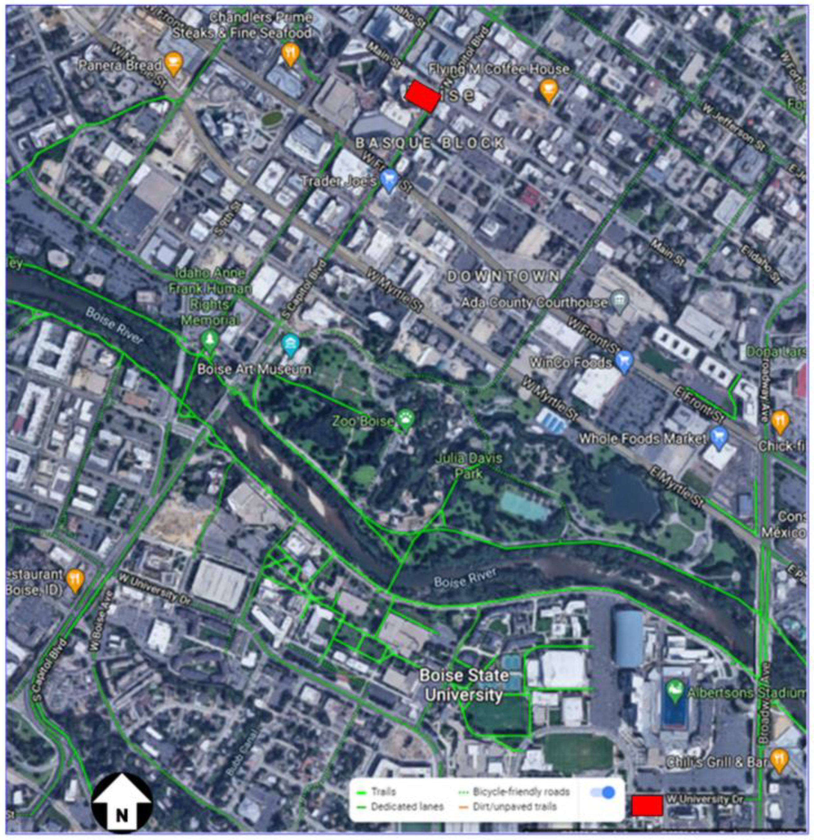
Figure 2.
Percentage of respondents choosing aerial tramway.


Table 1.
Response distribution.
| Affiliation | No Downtown Trip | Downtown Trip | Total |
|---|---|---|---|
| Faculty | 85 | 276 | 361 |
| Grad | 68 | 128 | 196 |
| Staff | 123 | 377 | 500 |
| UGLD | 53 | 408 | 461 |
| UGUD | 61 | 242 | 303 |
| Total | 390 | 1431 | 1821 |
Table 2.
Distribution of choices among the nine choice cases.
| Case | Number and Percentage Choosing Aerial Tramway | Case Description | |
|---|---|---|---|
| No Downtown Trip | Downtown Trip | ||
| 1 | 132 (34%) | 570 (40%) | Costlier but more convenient |
| 2 | 44 (11%) | 233 (16%) | Costlier but equally convenient |
| 3 | 5 (1%) | 44 (3%) | Costlier and less convenient |
| 4 | 252 (65%) | 972 (68%) | Same cost but more convenient |
| 5 | 203 (52%) | 788 (55%) | Same cost and convenience |
| 6 | 26 (7%) | 137 (10%) | Same cost but less convenient |
| 7 | 262 (67%) | 987 (69%) | Less costly and more convenient |
| 8 | 220 (56%) | 848 (59%) | Less costly but equally convenient |
| 9 | 64 (16%) | 276 (19%) | Less costly and less convenient |
Table 3.
Coefficient estimates for model without interaction variables.
| Coefficients | Estimate | Odds Ratio | Std. Error | z. Value | Pr...z.. | Sign. Code |
|---|---|---|---|---|---|---|
| (Intercept) | −0.70 | 0.50 | 0.099 | −7.06 | 1.63E-12 | *** |
| cost_convcase2 | −1.25 | 0.29 | 0.091 | −13.74 | 5.59E-43 | *** |
| cost_convcase3 | −3.07 | 0.05 | 0.163 | −18.85 | 3.07E-79 | *** |
| cost_convcase4 | 1.12 | 3.06 | 0.080 | 14.00 | 1.57E-44 | *** |
| cost_convcase5 | 0.64 | 1.89 | 0.078 | 8.23 | 1.80E-16 | *** |
| cost_convcase6 | −1.88 | 0.15 | 0.106 | −17.68 | 6.50E-70 | *** |
| cost_convcase7 | 1.28 | 3.58 | 0.081 | 15.69 | 1.66E-55 | *** |
| cost_convcase8 | 0.82 | 2.26 | 0.078 | 10.46 | 1.35E-25 | *** |
| cost_convcase9 | −1.05 | 0.35 | 0.087 | −12.00 | 3.74E-33 | *** |
| RoleGrad | 0.25 | 1.29 | 0.088 | 2.86 | 4.22E-03 | ** |
| RoleStaff | 0.16 | 1.17 | 0.065 | 2.40 | 1.65E-02 | * |
| RoleUGLD | 0.07 | 1.07 | 0.064 | 1.07 | 2.83E-01 | |
| RoleUGUD | 0.19 | 1.21 | 0.072 | 2.65 | 7.98E-03 | ** |
| ModeCar | 0.07 | 1.07 | 0.076 | 0.88 | 3.76E-01 | |
| ModeShuttle | 0.10 | 1.10 | 0.095 | 1.01 | 3.12E-01 | |
| ModeWalk | −0.20 | 0.81 | 0.091 | −2.25 | 2.48E-02 | * |
| Travel_time | 0.01 | 1.01 | 0.003 | 4.79 | 1.66E-06 | *** |
Sign. codes: “***” 0.001 “**” 0.01 “*” 0.05; null deviance: 16,519 on 12,365 degrees of freedom; residual deviance: 12,772 on 12,349 degrees of freedom.
Table 4.
Coefficient estimates for model with interaction variables.
| Coefficient | Estimate | Odds Ratio | Std. Error | z. Value | Pr...z.. | Sign. Code |
|---|---|---|---|---|---|---|
| (Intercept) | −1.06 | 0.35 | 0.14 | −7.48 | 7.65E-14 | *** |
| cost_convcaseY2 | −1.25 | 0.29 | 0.09 | −13.79 | 3.03E-43 | *** |
| cost_convcaseY3 | −3.08 | 0.05 | 0.16 | −18.90 | 1.09E-79 | *** |
| cost_convcaseY4 | 1.13 | 3.09 | 0.08 | 14.06 | 6.90E-45 | *** |
| cost_convcaseY5 | 0.64 | 1.90 | 0.08 | 8.27 | 1.35E-16 | *** |
| cost_convcaseY6 | −1.89 | 0.15 | 0.11 | −17.73 | 2.52E-70 | *** |
| cost_convcaseY7 | 1.29 | 3.62 | 0.08 | 15.76 | 6.00E-56 | *** |
| cost_convcaseY8 | 0.82 | 2.28 | 0.08 | 10.50 | 8.47E-26 | *** |
| cost_convcaseY9 | −1.05 | 0.35 | 0.09 | −12.04 | 2.31E-33 | *** |
| RoleGrad | 0.63 | 1.87 | 0.25 | 2.51 | 1.21E-02 | * |
| RoleStaff | −0.05 | 0.95 | 0.21 | −0.26 | 7.95E-01 | |
| RoleUGLD | 0.91 | 2.49 | 0.19 | 4.87 | 1.11E-06 | *** |
| RoleUGUD | 1.16 | 3.19 | 0.22 | 5.16 | 2.47E-07 | *** |
| ModeCar | 0.61 | 1.84 | 0.14 | 4.26 | 2.01E-05 | *** |
| ModeShuttle | 0.46 | 1.59 | 0.21 | 2.19 | 2.85E-02 | * |
| ModeWalk | −0.16 | 0.85 | 0.18 | −0.89 | 3.72E-01 | |
| Travel_time | 0.01 | 1.01 | 0.00 | 4.68 | 2.82E-06 | *** |
| RoleGrad:ModeCar | −0.69 | 0.50 | 0.27 | −2.52 | 1.17E-02 | * |
| RoleStaff:ModeCar | 0.06 | 1.07 | 0.23 | 0.28 | 7.79E-01 | |
| RoleUGLD:ModeCar | −1.10 | 0.33 | 0.21 | −5.33 | 9.90E-08 | *** |
| RoleUGUD:ModeCar | −1.23 | 0.29 | 0.24 | −5.07 | 3.95E-07 | *** |
| RoleGrad:ModeShuttle | −0.12 | 0.88 | 0.37 | −0.33 | 7.38E-01 | |
| RoleStaff:ModeShuttle | 0.21 | 1.24 | 0.29 | 0.74 | 4.61E-01 | |
| RoleUGLD:ModeShuttle | −0.83 | 0.44 | 0.27 | −3.02 | 2.51E-03 | ** |
| RoleUGUD:ModeShuttle | −1.19 | 0.30 | 0.32 | −3.71 | 2.07E-04 | *** |
| RoleGrad:ModeWalk | 0.45 | 1.56 | 0.36 | 1.26 | 2.09E-01 | |
| RoleStaff:ModeWalk | 0.65 | 1.91 | 0.27 | 2.35 | 1.86E-02 | * |
| RoleUGLD:ModeWalk | −0.57 | 0.56 | 0.24 | −2.38 | 1.71E-02 | * |
| RoleUGUD:ModeWalk | −0.44 | 0.64 | 0.30 | −1.49 | 1.37E-01 |
Sign. codes: “***” 0.001 “**” 0.01 “*” 0.05; null deviance: 16,519 on 12,365 degrees of freedom; residual deviance: 12,772 on 12,349 degrees of freedom.
Publisher’s Note: MDPI stays neutral with regard to jurisdictional claims in published maps and institutional affiliations. |
© 2021 by the author. Licensee MDPI, Basel, Switzerland. This article is an open access article distributed under the terms and conditions of the Creative Commons Attribution (CC BY) license (http://creativecommons.org/licenses/by/4.0/).
Share and Cite
MDPI and ACS Style
Khanal, M. Estimating Demand for a New Travel Mode in Boise, Idaho. Sustainability 2021, 13, 1209. https://doi.org/10.3390/su13031209
AMA Style
Khanal M. Estimating Demand for a New Travel Mode in Boise, Idaho. Sustainability. 2021; 13(3):1209. https://doi.org/10.3390/su13031209
Chicago/Turabian StyleKhanal, Mandar. 2021. "Estimating Demand for a New Travel Mode in Boise, Idaho" Sustainability 13, no. 3: 1209. https://doi.org/10.3390/su13031209
Note that from the first issue of 2016, this journal uses article numbers instead of page numbers. See further details here.