Influence of Complex Occupant Behavior Models on Cooling Energy Usage Analysis

Abstract

The behavior of building occupants has been studied by researchers for building control as well as for predicting energy use. In this study, we analyzed the effect of the application of single and complex behavior models on the simulation results of residential buildings. Two occupant behaviors—window opening and closing and air conditioner (AC) usage—were simulated, which are known to be interconnected. This study had two purposes: The first was to integrate data analysis tools (R in this study) and building simulation tools (EnergyPlus in this study) so that two behaviors with interconnectivity could be reflected in building simulation analysis. The second purpose was to apply the behavior models in residential buildings to an integrated simulation environment in stages to analyze their relative influence on the building energy and indoor environment. The results of the study prove that the application of complex behavior is important for research regarding the prediction of actual energy consumption. The results help identify the gap between reality and the existing simulation methods; thereby, they can help improve methods related to energy consumption analysis. We hope that this study and its results will serve as a guide for researchers looking to study occupants’ behavior in the future.

1. Introduction

Packaged air conditioners (ACs) are representative cooling systems that are commonly used in residential buildings as well as in small commercial buildings. The penetration rate of ACs in South Korea is expected to be 1.06 units per household in 2030 [1]. According to the growth trend of the AC market over the last few years, however, the penetration rate appears to have already exceeded this expectation. The increase in the use of ACs could be due to the increased demand for indoor environments driven by the effects of climate change and increasing disposable incomes. Despite the widespread use of ACs, the cooling load has not been included in the evaluation of the energy performance of residential buildings in South Korean systems, and residential devices for cooling are categorized as home appliances in most cases. However, in some East Asian countries with hot and humid climates, the impact of ACs on energy consumption is far too significant for them to be classified simply as home appliances [2,3,4].

Many researchers have used building simulation tools to predict the energy consumption of such cooling devices. Building simulation is performed for real-time control by predicting the energy consumption of a building or to review the effects of applied technologies. Although building simulation tools have different purposes, one of them is to simulate actual buildings. Such tools, however, have various uncertainties associated with their use, such as physical models, meteorological data, and input values, which create a deviation between the actual energy consumption of buildings and that obtained via simulations. There are various factors that cause such deviations, including occupant behavior (OB); hence, researchers have been studying this topic in order bring the simulation values closer to the actual values [5].

Before studies on the derivation of OB models were actively conducted, for most building simulations, values of variables related to OB, such as occupancy status, window opening/closing, and use of cooling and heating devices, were simply assumed (arbitrarily) and applied at the discretion of the simulation performer or based on guidelines for building energy performance analysis. If buildings have poor physical performance, such a simplification of OB information reduces the energy consumption, which may vary depending on OB. With the reinforcement of design standards for the levels of passive houses and with advances in analytical tools, however, OB has increasingly attracted the attention of researchers as the main factor that leads to a deviation between actual energy consumption and simulation results. For passive houses that were constructed between 1990 and 2018, the building performance that was predicted during the design stage was compared with the actual heating energy consumption, and analyses were performed. The analysis results revealed that OB accounted for a standard deviation of up to 50% [6]. Performing energy retrofitting using OB analysis helps in energy conservation; consequently, it results in excellent building energy performance [7]. OB analysis can also help in more accurately evaluating energy conservation measures, as it reduces the number of uncertain variables [8]. Additionally, OB is a main factor to consider when trying to understand the current energy consumption from the perspective of post-occupancy evaluation (POE). In other words, OB analysis is required to understand the current situation and to present a better direction [9]. As occupants have emerged as entities that determine the energy consumption of buildings [10], many related studies have been conducted with a focus on IEA Annex 66 “Definition and Simulation of Occupant Behavior in Buildings” and Annex 79 “Occupant-Centric Building Design and Operation”. According to a literature review on OB covering ten years (2009–2018) conducted by Balvedi et al., only three out of the ten most frequently cited studies were related to residential buildings. Although residential buildings also have an energy-saving potential, most studies have focused on commercial buildings, as the factors that determine behavior for residential buildings are relatively limited because of the difficulty with respect to data collection [11].

Studies on OB can be placed in three main categories: (1) identification of factors affecting behavior according to the research purpose and monitoring for data collection, (2) analysis of the collected data and development of behavior models, and (3) a simulation that applies the behavior models. In general, these categories are not covered in one study, but the scope varies depending on the purpose of the study. Studies on the operation of a building’s predicted OB consider physical factors and time, which are collected through monitoring. Some studies introduced mathematical models to predict the window opening/closing behavior, which compared the measured data with the simulation data, and reported that behavior models could reproduce the general behavior of actual occupants [12,13,14]. Meanwhile, these results could be derived because the large influence of AC operation on the window opening/closing behavior was excluded [15]. OB changes indoor environments, and the changed indoor environments affect OB. Consider a simple example wherein an occupant decides to open a window in an indoor environment and takes action; the outside air comes inside and changes the indoor environment. The changed environment determines the next action of the occupant. The window opening behavior of the above example may affect the usage behavior of the AC or blinds of the occupant. Imagawa et al. conducted an analysis by integrating the window and AC on/off behavior. They predicted the behavior based on the outdoor temperature and analyzed the combined effect of complex behavior [16,17]. Cong Yu et al. reflected the OB information derived through a survey in a building energy simulation for residential buildings in Hong Kong to improve the accuracy of results; they also recommended that window and AC operation must be considered together in OB [18].

Then, will it be possible to reflect OB models that are complexly related to indoor environments in building energy analyses? Hong et al. developed an ontology that provides a common descriptive language capable of observing, modeling, and simulating OB in building simulations over many years of research [19,20]. Based on this, they provided a standardized structure for describing OB and integrated behavior with building energy modeling and a functional mock-up unit (FMU) by devising an obXML (occupant behavior extensible markup language) schema that includes drivers, needs, actions, and systems (DNAS). They also provided a platform that can be used for operation scenarios of lighting, windows, and heating, ventilation, and air conditioning (HVAC) using an OB modeling tool that integrated EnergyPlus and obFMU [21]. Research on the methodologies for deriving OB models from collected data and applying such models to building simulation tools is currently underway. The importance of linking buildings with occupants by implementing OB when performing building simulations is increasing along with the importance of smart building systems.

This study was conducted with a focus on the effect of the application of behavior models (single or complex) on building simulation results. Thus, this study had two purposes, as shown in Figure 1. The first was to integrate data analysis tools and building simulation tools so that two behaviors with interconnectivity could be reflected in building simulation analysis. For behavioral models that can be predicted by mathematical models, behavioral simulation can be performed using a single tool (EnergyPlus in this study). However, a new approach is required to apply the behavior predicted by machine learning methods to building simulations. In addition, when conducting behavioral simulations in a co-simulation environment, the timestep must also be reviewed, which has become an issue in buildings with high heat capacity because the behavior is predicted by the behavior model based on the timestep. Therefore, the proper timestep is discussed. The second purpose was to apply the behavior models in residential buildings to an integrated simulation environment in stages to analyze their relative influence on the building energy and indoor environment. In this process, the impact of applying a single behavior model and the influence of applying a composite behavior model were analyzed, and in the case of the complex behavior model, a case analysis was conducted according to the behavior preferred by the residents.

2. Materials and Methods

2.1. Occupant Behavior (OB)

Among the behaviors of occupants, occupant presence is a behavior that must be determined before the occurrence of other behaviors. Because other behavior may occur based on occupant presence, many studies attempted to judge/predict occupant presence [22,23]. The effect of predicting the presence status on the building energy/environment may vary depending on the use of each building. In commercial buildings, multiple zones are generally controlled using a single heat source facility; hence, the accurate prediction of the occupant presence status may result in significant energy savings. However, the occupant presence status in residential buildings is not as significant because the living spaces of occupants are generally relatively small, and the number of occupants is almost fixed.

The main behavior related to ACs will be turning the AC on/off and the adjustment of the temperature. One more important OB is the window opening/closing behavior. The window status determined by OB may affect the AC on/off status, which may conversely affect the window status. In other words, these two behaviors must be simulated together because they affect each other. In this study, behavioral information and changes in cooling energy consumption were simulated according to the reflection of these two behaviors.

2.1.1. AC On/Off

Numerous studies on AC usage behavior have been conducted to analyze influencing factors, which are the preliminary stages of deriving behavior models. The results of previous studies showed that they were mostly conducted with a focus on the physical environmental parameters (especially indoor and outdoor temperatures) among the seven categories that determine behavior (environmental, time-related, contextual, physiological, psychological, social, and random) [24]. Among the studies that have been published since 2014 when active research on OB started, few predicted the AC usage behavior of occupants in residential buildings using physical elements as variables. The AC usage prediction models presented in previous studies are based on various forms, such as a Sigmoid function, Weibull distribution, or operation probability by time [2,3,25].

AC usage behavior is significantly affected by geographical, cultural, and social elements. Therefore, this study attempted to use models derived in South Korea. Few studies have focused on the AC usage behavior of occupants in South Korea, and only one study predicted the on/off status using the Random Forest (RF) algorithm and a support vector machine (SVM). Machine learning methods, such as RF and SVM, are used not only for building-related predictions, but also in various areas, and their excellence as prediction algorithms has been verified by many researchers [26]. RF, an ensemble technique, overcame the shortcomings of decision trees by bagging (or bootstrap aggregating). Bagging is a method used to overcome bias and variance, which are the two components of learning errors. It determines the prediction results by generating N prediction models from training data through random sampling and allowing the individual prediction models to vote. Next, SVM is an algorithm that finds the optimal decision boundary so that the margin for grouping data can be maximized. The large margin means that data can be classified in a stable manner, even when new data are added in the future. SVM introduces a parameter cost (C) to allow errors caused by outliers, and the complexity and generalization performance of the model are determined by the C value. These learning algorithms have been actively used in research related to energy prediction [27,28,29]; however, there are not many cases that have focused on behavior prediction.

Building energy models are required in various cases, such as the examination or optimization of the efficiency of building retrofitting and the preparation of control measures. If machine learning methods must be linked in this instance, the model cannot be solved using a single tool. In other words, it is necessary to construct a co-simulation environment to connect such algorithms with building energy simulations. In this study, the co-simulation of R, a data analysis tool, and EnergyPlus, which is a building energy simulation tool, was performed. The details of the co-simulation are discussed in Section 2.2.

2.1.2. Set Temperature Adjustment

The set temperature has a considerable influence on the calculation of the load of a building. Moon and Han (2011) analyzed the energy-saving effect according to the set temperature under different climatic conditions for typical single-family houses in a cold region (Detroit) and a hot and humid region (Florida) and found that a set temperature of 1 °C caused cooling energy differences of 10.3% and 7.7%, respectively. This shows that thermostat settings have a significant impact on the cooling and heating energy consumption of residential buildings [30].

In South Korea, the cooling set temperature generally applied for building energy analysis is 26 °C. This recommended value is significantly different from the temperatures actually set by occupants. Although public buildings must follow this recommended temperature, the set temperature in residential buildings varies depending on the preferences of occupants. Sun et al. (2017) varied the set temperature according to the energy use propensity of occupants in a study that analyzed the energy measure application effect [31]. Mun et al. (2018) collected signals from remote controls of ACs with Arduino, analyzed the set temperature among the collected information, and concluded that it is difficult to predict the set temperature because the propensity of occupants is reflected in it [32]. In addition, Tushar et al. (2017) designed a temperature control policy for ACs in shared spaces [33]. This verified that temperature control has an important effect on energy determination. Predicting the set temperature is not easy because it is linked with the occupants’ propensities and behaviors (including the various factors that affect behavior, such as systems and income levels). Wang et al. (2016) reported on not only the indoor temperature and humidity, but also the feedback of occupants regarding real-time comfort in predicting the set temperature of cooling/heating devices [34]. Based on this background, this study considered that predicting the set temperature is impossible and judged that assuming a normal distribution is the most reasonable at the current level by referring to a previous study [35].

2.1.3. Window Open/Closed State

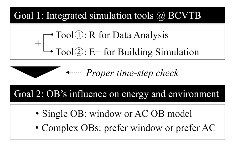
In this study, a regression model was used to model the window opening/closing status. Logistic regression (LR) is a probabilistic classifier for predicting the binomial or polynomial results by fitting conditional probability to a logistic function. A logistic function can be understood from the same viewpoint as the Bernoulli trials, as shown in Equation (1), and μ(x) in Equation (2) is a logistic function. Differently from the linear regression model, which represents a linear relationship between probability and predicted variables, the LR model has an advantage in predicting the upper and lower intervals of variables. Researchers consider the LR model to be the most appropriate for describing discrete behaviors, such as the opening/closing of windows [36,37,38,39,40,41,42]. The LR model can be generalized into a linear function, as expressed in Equation (3).

$$\mathrm{P}\left(y|x\right)=\mu {\left(x\right)}^y{\left(1-\mu \left(x\right)\right)}^{1-y}$$

(1)

$$\mathsf{\mu }\left(x\right)=\frac{1}{1+e^{-{\theta }^{T}x}}=\frac{e^{X\theta }}{1+e^{X\theta }}=\mathrm{P}(y=1|x)$$

(2)

$$\log \left(p_i\right)=\ln \left(\frac{p_i}{1-p_i}\right)={\mathsf{\beta }}_0+{\mathsf{\beta }}_1{x}_{1,i}+{\mathsf{\beta }}_2{x}_{2,i}+\dots +{\mathsf{\beta }}_m{x}_{m,i}$$

(3)

where p_i is the probability of the occurrence of behavior (%), β_m is the LR coefficient, and x_m,i is a variable or factor of the inducement of behavior(s). The LR model can be easily applied to building energy simulation [43].

2.2. Co-Simulation

Advances in research contents required by the building sector have also led to advances in the tools used; in this process, researchers have conducted various studies through co-simulation [44,45,46,47,48]. In particular, because of the growing need to utilize building energy or environmental information data, it is necessary to integrate data with building energy simulation.

There are two coupling types: internal coupling, which fuses one model with another and has only one solver, and external coupling, which fuses different models with their own solvers and exchanges data with other solvers. Internal coupling requires high development and maintenance costs as well as considerable computation time because the integration must be performed with each program’s source code. By contrast, external coupling is easy to implement if only the interface of each program is understood instead of analyzing the source code, and it can utilize distributed computing [49]. External coupling can be classified into static and dynamic synchronization according to the synchronization system and into one-way and two-way data exchange according to the data exchange direction. One-time data exchange for the entire simulation is known as static synchronization, and multiple data exchanges are referred to as dynamic synchronization. If only one program provides data to another, it is referred to as one-way data exchange. If data are exchanged between two programs, the program is referred to as two-way data exchange [49].

In this study, two processes were repeatedly simulated. First, OB was learned and predicted. The predicted behavior was then input into a building energy analysis tool to derive the indoor thermal environment and energy consumption. R [50], which performs object-oriented programming, was used to learn and predict OB, and EnergyPlus [51], a dynamic building energy analysis tool, was utilized to derive the indoor thermal environment and energy consumption.

In the case of this study, the AC operation status was predicted using a machine learning algorithm (i.e., RF), and the indoor thermal environment was affected by two behaviors—window opening/closing and AC on/off status. Therefore, a simulation that considers these is required. In other words, the simulation must be performed while the AC operation prediction information and information on window opening/closing and AC on/off status are exchanged at each timestep of the simulation (EnergyPlus). In addition, the indoor thermal environment and energy consumption are simulated by reflecting the OB predicted at each timestep. Among the results, the indoor thermal environment information must be used again to predict the OB at the next timestep. These two processes are similar to the ping-pong [52] method, in which the next timestep is reached while the results are being exchanged. Conventional building energy analysis tools, however, cannot exchange research results of different types while performing simulations. This is because simulations are performed after entering all the variables, and it is extremely difficult to add or modify variables while a simulation is being performed. Therefore, to address this problem, an environment for co-simulation must be developed so that the research results of different types can be exchanged while the simulation is being performed. Co-simulation aims to overcome or complement these shortcomings by coupling two or more simulation tools and software programs and utilizing their benefits [53]. The building control virtual test bed (BCVTB) provides a middleware environment for co-simulation construction [54]. In this study, for cases where integration with data analysis tools is required, a co-simulation environment was constructed, so that the next timestep could be reached while the results derived by the two simulation tools were exchanged on the BCVTB. In other words, we implemented R for predicting AC and window operation behavior and EnergyPlus for analyzing the indoor thermal environment and energy consumption on BCVTB. The two tools are independently simulated on BCVTB; however, the input and output of each tool are exchanged. Therefore, the simulation of R predicts the behavior at the next timestep by reading and utilizing the variables derived from EnergyPlus. In addition, EnergyPlus reads the behavior information predicted by R and reflects it in the AC operation schedule of the EnergyPlus input file and the window opening factor to perform the simulation. Therefore, in this study, co-simulation corresponds to external coupling, which is a dynamic synchronization scheme that performs two-way data exchange, because the result data of the two programs are exchanged at each timestep. In addition, the variability of the model must be considered in behavior research. When there are many occupants or constant changes, like in hotels, the use of fixed machine learning algorithms has limitations. Therefore, the algorithms must be updated, such as by reinforcement learning. As this study targeted a single household and was based on the premise that the subject of the behavior did not change, the use of a single machine learning algorithm did not cause any significant problems.

3. Building Energy Simulation with OB

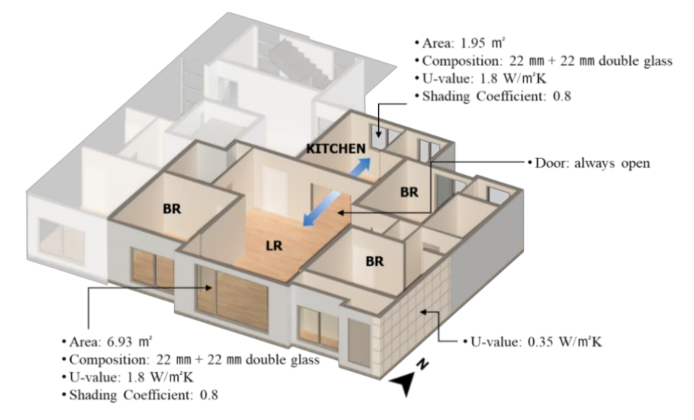
3.1. Overview of the Building Energy Simulation

Figure 2 shows an overview of the reference unit [55]. The area of the window in the living room is 6.93 m², and that of the kitchen is 1.95 m²; the floor plan was favorable for cross-ventilation. Generally, there are no interior walls between the kitchen and the living room in South Korea. Therefore, AC usage in the living room affects the air state in the kitchen. To reflect this, a dummy door between the living room and the kitchen was modeled, and the air in the living room and kitchen was allowed to be mixed by assuming that the door was always open through an AirFlowNetwork (AFN) in EnergyPlus. Because the other rooms were separated by doors, the cooling area of the AC was 58.27 m² (41.75 m² for the living room + 16.52 m² for the kitchen). The airtightness level of the unit was adjusted so that the infiltration amount derived by AFN could be 0.15 ACH. This value was obtained by applying a windproof coefficient of 0.05 to the infiltration amount of 3.0 ACH at n50. The typical meteorological year (TMY) data of Seoul (1981–2010) were used as weather data for the simulation, and the simulation period was from August 1 to 7.

Table 1. Standard annual weather data during the simulation period.

	Dry-bulb Temperature [°C]	Relative Humidity [%]	Solar Radiation [W/m3]
Average	22.8	72.6	428.2
Min.	11.7	43.4	0.0
Max.	31.7	95.5	992.6
Median	23.0	75.7	334.3

summarizes the standard annual weather data during the simulation period. Next, it was assumed that occupants were always present in the living room or kitchen to maximize the behavior expression possibility, i.e., to minimize the influence of the occupant presence status on the simulation results of other behaviors.

3.2. Applying OB Models for Building Energy Simulation

In this study, the window operation model and AC on/off model derived from the same raw data were used. OB varies by country over a broad scope and among household members over a narrow scope. As mentioned previously [5], the cultural and socio-economical characteristics of occupants as well as the influence of the climate of the corresponding region are reflected in behavior models. Therefore, a logit model for window operation and an AC on/off model using the RF algorithm derived from the same raw data were utilized [32].

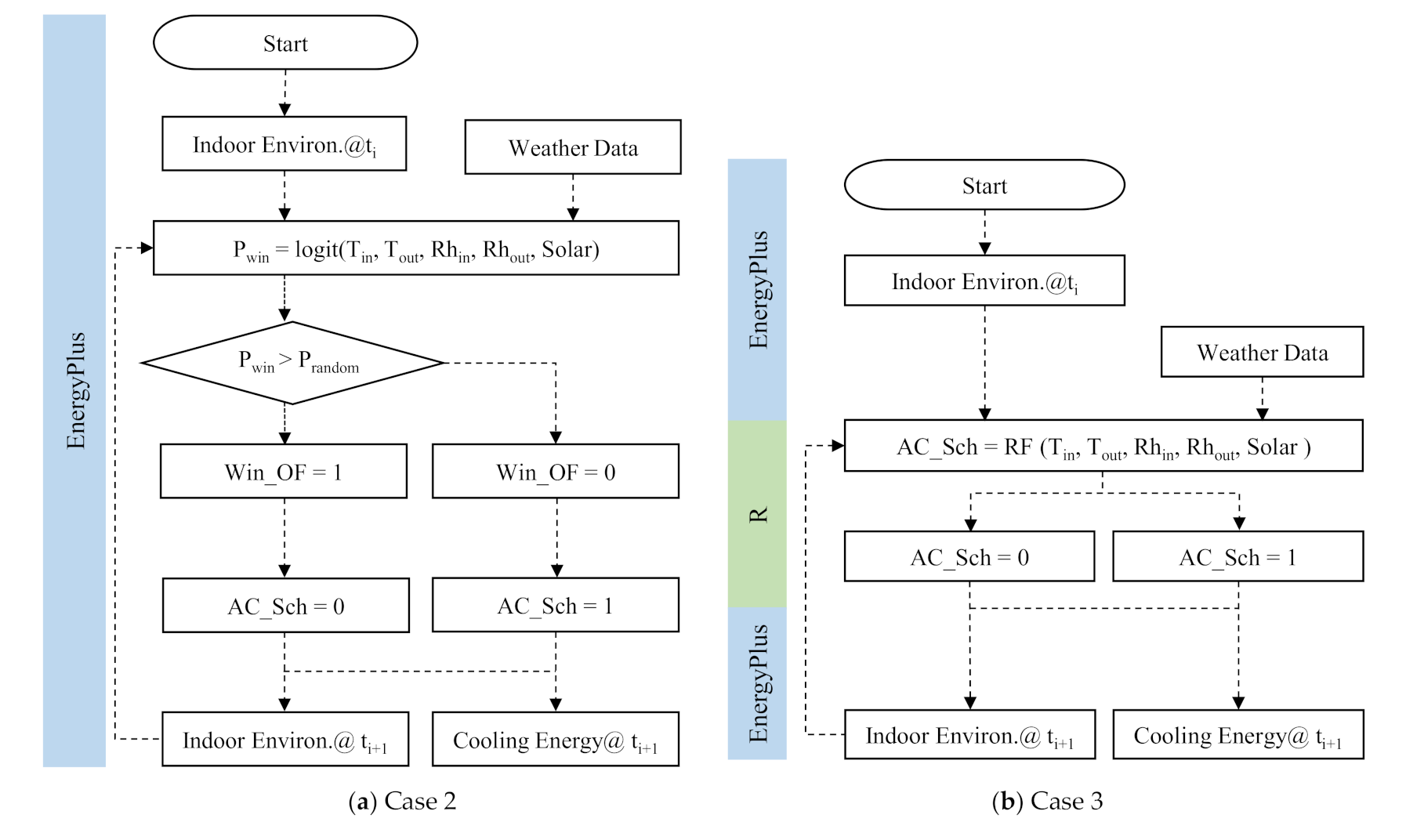
3.2.1. Logit Model for Window State

The initial variables of the logit model for predicting window opening/closing were indoor temperature and humidity, outdoor temperature and humidity, and horizontal total solar radiation. The data were preprocessed every 10 min before use. Equation (4) shows the window opening/closing behavior model derived through the glm function of R [32].

$$\ln \left(\frac{P_o}{1-P_o}\right)=-0.778+0.0086T_{in}-0.371T_{out}+0.147R{h}_{in}-0.0487R{h}_{out}-0.004\log \left(Solar\right)$$

(4)

where T_in is the indoor temperature (°C), Rh_in is the indoor relative humidity (%), T_out is the outdoor temperature (°C), Rh_out is outdoor relative humidity (%), and Solar is the horizontal solar radiation (W/m²).

In this study, the logit model was simulated using two methods depending on the analysis case. The model was implemented in the EnergyManagementSystem class of EnergyPlus when only the window opening/closing behavior model was applied, and in R when both the AC model and the behavior model were applied. The details are described in Section 3.3.

3.2.2. RF Model for AC State

The AC operation model used here makes predictions based on the RF algorithm. The number of trees (ntree) was 953, and the number of features in each tree (mtry) was 5. In this instance, the OOB (Out-Of-Bag) error was 1.01%, the F-measure by cross-validation was 0.9, and Cohen’s Kappa was 0.83, indicating that the model had a high prediction rate. The details regarding the derivation process and verification of the model are described in [32].

3.3. Definition of Cases

As described in Section 1, one of the main factors affecting the energy consumption of ACs is their set temperature, which is determined by occupants. When behavior models are not reflected, i.e., for models in which all conditions for simulation are identical, the tendency of the energy consumption change can be predicted in a problem that has only the set temperature as a variable. By contrast, when performing simulation by applying behavior models, it is impossible to predict the change in energy consumption because the simulation conditions at each timestep may vary depending on the set temperature. Therefore, the set temperature was applied as a variable for case classification in this study. In 2018, Mun et al. found that the set temperature information collected through the infrared signals of the AC remote controls included cases in which specific set temperatures were preferred by occupants and cases with various set temperatures. It was confirmed that the latter set of temperature data had the characteristics of normal distribution [32]. Zhou et al. conducted research on the AC usage behavior of occupants and assumed that the set temperature had a normal distribution [25]. As such, in this study, the set temperature was applied such that 24, 26, and 28 °C could be the average temperatures (minimum of 18 °C and maximum of 30 °C).

Next, four cases were established depending on the reflection of the window opening/closing and AC usage behavior.

Table 2. Analysis cases depending on the reflection of the window and air conditioner (AC) behavior.

Case	Input Method		Description	Figure 3
	Window	AC
1	Closed	Off	The windows are closed at all times, and the AC always operates at the Tset.	-
2	Behavior model	Off	When the windows are opened, the AC is off, and the AC operates at the Tset when the window is closed.	(a)
3	Closed	Behavior model	The windows are closed at all times, and the AC operation status is predicted and reflected by RF.	(b)
4	Behavior model 1	Behavior model 2	The occupant first determines window status and then determines the AC on/off status when the window is closed.	(c)
5 *	Behavior model 2	Behavior model 1	The occupant first determines AC on/off status and then determines the windows status only when the AC is off.	(d)

* During the simulation, the behavior at timestep t_i affects the determination of the behavior at timestep t_i+1. Because these effects occur continuously during the simulation period, it is necessary to analyze the behavior determination order. The OB implementation of these sequences can be linked with the propensity of the corresponding occupants.

summarizes the simulation cases analyzed in this study; Figure 3 shows the process of each case.

4. Results and Discussion

4.1. Effects of the Timestep on OB Simulation

EnergyPlus recalculates the energy/environment at each timestep, which is a discrete bin of time. According to the input and output reference [51] of EnergyPlus, timestep 4 (15 min interval) is recommended for deriving stable results without a significant increase in the computation time. Tabares-Velasco reported that the initial dynamic behavior of a wall was completely inaccurate when the timestep was 1, and that responses that were fast enough to implement the actual phenomenon were observed when the timestep was higher than 4. They also suggested that the system timestep should preferably be 6 or higher (10 min or less) to analyze the cooling peak [56]. For all simulation tools, including EnergyPlus, the timestep generally has only the meaning of discrete time to interpret energy balance equations. In simulations that include behavior models, however, the timestep also has the meaning of the minimum time, in which the behavior determined in the previous timestep is maintained in addition to its original meaning. Therefore, a more appropriate timestep must be selected for sudden changes in indoor conditions or for behavior that has a considerable influence on energy.

According to a survey on the existing literature, there are not many cases in which behavior models have been implemented in simulations. In addition, no cases examined the influence of the timestep in the process. In this study, an additional simulation was performed for Case 4 (the AC status is predicted when the window status prediction result is closed) to analyze the influence of the timestep on the simulation of behavior models. In addition, to analyze the change according to the set temperature, the simulation results are summarized in

Table 3. Simulation results according to the timestep.

	OB		Timestep 1 (60 min)	Timestep 2 (30 min)	Timestep 4 (15 min)	Timestep 6 (10 min)
24 °C	Window	Daily window OB frequency [-]	3.4	6.3	8.7	13.0
		Daily open state time [h/d, (%)	4.4 (18.5)	4.8 (19.9)	4.4 (18.2)	4.2 (17.5)
		Duration of one-time opening [h/d, (hmax)]	1.3 (4.0)	0.8 (3.0)	0.5 (5.3)	0.3 (2.3)
	AC	Daily AC OB frequency [-]	1.4	2.3	4.7	7.3
		Daily operation time [h/d,(%/d)]	3.3 (13.7)	3.1 (13.1)	3.1 (13.1)	3.5 (14.5)
		One-time operation time [h, (hpeak)]	2.3 (7.0)	1.4 (7.0)	0.7 (4.0)	0.5 (2.8)
		Daily energy usage [kWh/d]	5.2	5.5	5.2	5.3
		Energy usage peak [kWhpeak/h]	3.2	3.4	1.8	1.4
26 °C	Window	Daily window OB frequency [-]	3.6	5.9	8.6	14.4
		Daily open state time [h/d, (%)	4.9 (20.2)	4.6 (19.1)	4.5 (18.6)	4.4 (18.5)
		Duration of one-time opening [h/d, (hmax)]	1.4 (5.0)	0.8 (4.0)	0.5 (3.8)	0.3 (3.2)
	AC	Daily AC OB frequency [-]	1.6	2.9	4.0	5.7
		Daily operation time [h/d,(%/d)]	3.7 (15.5)	3.9 (16.1)	4.1 (17.3)	3.9 (16.1)
		One-time operation time [h, (hpeak)]	2.4 (4.0)	1.4 (2.5)	1.0 (6.5)	0.7 (4.8)
		Daily energy usage [kWh/d]	4.9	5.0	5.00	4.7
		Energy usage peak [kWhpeak/h]	2.9	3.1	2.4	1.9
28 °C	Window	Daily window OB frequency [-]	1.6	4.7	9.4	10.7
		Daily open state time [h/d, (%)	2.4 (10.1)	4.4 (18.5)	4.18 (17.4)	3.9 (16.5)
		Duration of one-time opening [h/d, (hmax)]	1.6 (4.0)	0.94 (6.5)	0.44 (3.5)	0.4 (2.3)
	AC	Daily AC OB frequency [-]	1.1	2.3	3.0	3.9
		Daily operation time [h/d,(%/d)]	4.3 (17.9)	3.9 (16.1)	4.3 (17.7)	4.1 (17.2)
		One-time operation time [h, (hpeak)]	3.8 (12.0)	1.7 (5.0)	1.4 (5.0)	1.1 (6.0)
		Daily energy usage [kWh/d]	4.1	3.8	3.9	3.7
		Energy usage peak [kWhpeak/h]	2.9	2.7	1.9	1.7

.

The simulation results based on the timestep show that the window OB frequency increased, but the duration of one-time opening decreased as the timestep increased. Consequently, the average window opening time was similar and was in the 18.15–19.94% range. This tendency was similar when the set temperatures were 24 and 26 °C. In addition, as the timestep increased, the AC OB frequency increased, but the one-time operation hours decreased. In other words, the same patterns as those of the window behavior analyzed earlier were observed.

When the energy consumption was examined according to the timestep, no significant differences were observed in the energy consumption, as the timestep varied at each set temperature. The peak value, however, exhibited a large difference according to the timestep, and this difference increased as the set temperature decreased. These results were similar to the results of the research on the timestep presented in [56].

Overall, we showed that the increase in the timestep affected the behavior frequency, but it did not have a significant effect on the window opening time and energy consumption. We confirmed, however, that the timestep must be carefully selected when the capacity of a facility has to be calculated or the peak load of the target building has to be analyzed. Because the peak load may increase when the timestep is low, the timestep must be selected considering various conditions, such as computer specifications and simulation time. By contrast, when behavior models are applied to the seasonal load analysis rather than the peak load analysis, the application of timestep 1 appears to be sufficient.

The results reviewed in this study are both behavioral information and energy data of behavioral models that are reflected in building energy analysis. In addition, because the computing time must be considered during co-simulations, a case study was conducted based on timestep 4.

4.2. OB Applicability

4.2.1. Window Operation

Table 4. Behavior information from the simulation results of the cases that reflected the window operation model.

		Case 2			Case 4			Case 5
Set Temperature [°C]		24	26	28	24	26	28	24	26	28
OB frequency	Daily avg.	1.9	1.6	1.7	8.7	8.6	9.4	6.4	7.9	7.9
Open State	Percentage [%]	54.9	53.9	53.9	18.2	18.6	17.4	16.2	14.7	16.7
	Daily avg. [h/day]	13.2	12.9	12.9	4.4	4.5	4.2	3.9	3.5	4.0
Duration of one-time opening	Max [h]	14	14.3	14.3	5.3	3.8	3.5	4.3	3.3	5.5
	Avg. [h]	7.1	8.2	7.5	0.5	0.5	0.4	0.6	0.5	0.5

summarizes the window opening/closing behavior information from the simulation results of cases that reflected the window operation model. In Case 5, the model in which AC operation was determined first, the window opening/closing frequency was lower than that in Case 4 by 1.52 times because the window opening/closing was predicted only when the AC was off. The window open time was approximately 50% (approximately 13 h per day on average) of the simulation time for Case 2 (the simulation times were 4.3 and 3.8 h for Cases 4 and 5, respectively), indicating that the window was open over a relatively short period of time for Cases 4 and 5. In the case of the time in which one window opening behavior lasts, Cases 4 and 5, which considered both the window opening/closing and AC behaviors, provided a short duration as a result. Next, the simulation results showed that the window opening/closing behavior with the set temperature had no obvious tendencies because the indoor temperature has a positive effect on the window opening/closing probability (the probability of opening the window increases as the indoor temperature increases) in the window operation model applied in this study (Equation (4)); however, it has an insignificant effect on the final behavior determination probability because the standardized coefficient is 0.0086. If the influence of the indoor temperature is large in the window operation model, a tendency may occur. This, however, can be predicted only for Case 2, in which only the window operation model was applied.

In Case 4, unlike Case 2, when the prediction result of the window operation model is “closed (opening factor = 0)”, the process for predicting the use of AC continues. When it is “opened (opening factor = 1)”, however, AC usage is interrupted, and the indoor environment is adjusted by natural ventilation (the determination of AC occurs first in Case 5). While the air change rate was 0.15 ACH on average for Cases 1 and 3, which did not apply the window operation model, it ranged from 2.1 to 5.9 ACH for Cases 2, 4, and 5, which used natural ventilation depending on the set temperature. The air exchange can be a benefit or a loss for the cooling load depending on the indoor/outdoor air conditions. To analyze the effect of applying the window operation model on the cooling load, the window opening/closing status predicted by the simulation, indoor/outdoor air condition, and air change rate were utilized (Equations (5)–(9)), and the results are shown in Figure 4. The influence of window opening and closing behavior on the cooling load was calculated using the amount of ventilation while the windows were opened and the indoor and outdoor air conditions at that time. We used Equations (5)–(9), the opening and closing conditions, the amount of ventilation, the indoor and outdoor dry bulb temperatures, and absolute humidity, which are the simulation results. In the case of the target unit, because the living room and kitchen are one space, the effects on the two spaces were analyzed together.

$$V_{window}=ACH·V$$

(5)

$$Q_{sensible}=\sum \left(\rho ·C_p·\left(T_{in}-T_{out}\right)\right)$$

(6)

$$Q_{latent}=\sum \left(\rho ·L·\left(x_{in}-x_{out}\right)\right)$$

(7)

$$Q_{LR}=\left(Q_{s,lr}+Q_{l,lr}\right)·V_{window,lr}$$

(8)

$$Q_{kit}=\left(Q_{s,kit}+Q_{l,kit}\right)·V_{window,kit}$$

(9)

where ρ is the density of air (1.2 kg/m³), C_p is the specific heat of air at constant pressure (1.01 kJ/kg‧K), L is the latent heat of vaporization of water at 0 °C (2501 kJ/kg), V is the air volume (m³), ACH is the air change rate (1/h), V_window is the air volume exchanged through the window (m³), Q is the cooling effect (W), Q_s is the sensible heat cooling effect (W), and Q_l is the latent heat cooling effect (W).

The net cooling effect (net CE, blue bars) through natural ventilation during the window opening time was positively analyzed from a minimum of 124 kWh to a maximum of 356 kWh during the simulation period. In all cases, however, there were instances in which the cooling load was increased by window opening/closing. The increase in the cooling load (adverse CE, black dotted lines) by the window became lower as the AC model was applied and the set temperature increased. The change in adverse CE according to the set temperature was the largest for Case 2, which applied only the window operation model, and the smallest for Case 4, which determined AC status after determining the opening/closing of the window. In Case 2, an adverse CE was observed, which was as high as 105 kWh, when the set temperature was 24 °C. In Cases 4 and 5, by contrast, the window opening/closing behavior was favorable for natural cooling. This is because the conditioned air exchanged heat with the outside air, which had a probabilistically high temperature, because of the opening/closing of the window when the set temperature was low. When the set temperature was high, on the contrary, the opening/closing of the window had a positive natural ventilation cooling effect because it was highly likely that the outside air had a lower temperature than the inside air.

The results show that the cooling effect through natural ventilation cannot be interpreted by the air change rate through the window. In Case 2, the air change rate increased along with the natural cooling effect as the set temperature increased. However, in Cases 4 and 5, which also applied the AC behavior model, this tendency could not be applied. When the set temperatures were 26 and 28 °C in Case 4, the air change rate through the window was the same, but the resulting net CE showed a difference of 55 kWh. In the case of 24 °C of Case 4 and 28 °C of Case 5, the air change rate was also the same; however, the net CE of Case 5 with a higher set temperature was found to be 66 kWh higher.

4.2.2. AC Usage

Table 5. Information regarding AC operation behavior based on the simulation results by case.

	Tset [°C]	Daily AC on/off Frequency [-]		One-Time Operation Time [h]		Daily Operation Time [h/d, (%)]
		Fan	Coil	Fan	Coil	Fan	Coil
Case 1	24	0.14	9.71	168	2.17	24 (100)	21.1 (87.8)
	26	0.14	13.00	168	1.53	24 (100)	19.9 (82.7)
	28	0.14	16.71	168	1.09	24 (100)	18.3 (76.2)
Case 2	24	1.71	3.57	6.31	2.87	10.8 (45.1)	10.3 (42.7)
	26	1.43	4.71	7.75	2.03	11.1 (46.1)	9.6 (39.9)
	28	1.57	6.43	7.05	1.17	11.1 (46.1)	7.5 (31.4)
Case 3	24	3.00	3.00	1.43	1.43	4.3 (17.9)	4.3 (17.9)
	26	2.29	2.29	2.09	2.09	4.8 (19.9)	4.8 (19.9)
	28	1.71	1.86	3.06	2.81	5.3 (21.9)	5.2 (21.7)
Case 4	24	4.71	4.71	0.67	0.67	3.1 (13.1)	3.1 (13.1)
	26	4.00	4.00	1.04	1.04	4.1 (17.3)	4.1 (17.3)
	28	2.00	3.00	2.29	1.42	4.8 (19.1)	4.3 (17.7)
Case 5	24	3.57	3.57	1.06	1.06	3.8 (15.8)	3.8 (15.8)
	26	3.29	3.29	1.34	1.34	4.4 (18.3)	4.4 (18.3)
	28	1.57	2.00	3.00	2.29	4.7 (19.6)	4.6 (19.1)

summarizes the information on AC operation behavior using the simulation results by case. First, in Case 1, the daily average operation time of the fan was 24 h because the AC behavior model was not reflected, and its one-time operation time was found to be 168 h (7 days) because it was not turned off during the simulation period. For the coil, by contrast, as the set temperature increased, the behavior frequency increased as the duration of the cooling load decreased, but the one-time operation time and daily average operation time decreased as the cooling load decreased. In Case 2, which reflected the window opening/closing behavior, the daily average operation time of the fan can be obtained by subtracting the window opening time from 24 h because the fan is off when the window is on, and it is on when the window is off. In Case 3, the window was always closed, and the AC was operated according to the results predicted by RF. Therefore, the on/off frequency of the fan and coil was high; however, their one-time operation times were short when the set temperature was low. In Case 4, window opening/closing was predicted first, and AC on/off was predicted and reflected in the building energy simulation only when the window was closed. In this case, as the set temperature increased, the on/off frequency of the fan and coil decreased, but their one-time operation times increased. In Case 5, where the AC’s on/off state was determined first, the same patterns that were also observed in Case 4 were observed. In Cases 3, 4, and 5, the coil operation time increased as the set temperature increased. This could be because the AC was operated over a long period of time to bear the instantaneously high load when it was turned on. In addition, in Cases 3, 4, and 5, which reflected the AC behavior model, the fan and the coil exhibited the same operation hours when the set temperatures were 24 and 26 °C. This means that the AC operation timing was the same as the timing of the cooling load occurrence. When the set temperature was 28 °C, however, the operation hours of the fan were longer than those of the coil because the AC could be operated even though the indoor temperature was lower than 28 °C.

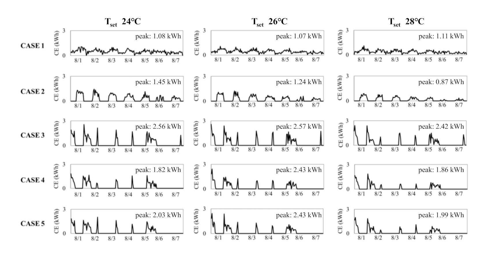
4.2.3. Cooling Energy Usage

The difference in the behavior information according to the application scope of the behavior models discussed above eventually leads to the difference in the energy consumption. Figure 5 shows the energy consumption according to the set temperature.

In all cases, the daily average energy consumption decreased as the set temperature increased. Each case, however, exhibited different trends. The case that exhibited the largest reduction in energy consumption because of the increase in the set temperature was Case 2, which reflected only the window opening/closing behavior. In other words, when the energy consumption was derived by applying only the window opening/closing behavior, the importance of the set temperature could be excessively emphasized. In Cases 3, 4, and 5, in which the AC operation status prediction model was applied, the change rate (Δ) was lower than 1. When complex behavior was applied, higher reduction rates were observed compared to those in Case 3, in which only the AC behavior was applied, but lower reduction rates were shown compared to Case 1, in which no behavior was applied. In addition, the reduction tendency was completely linear when no behavior was applied. When behavior was applied, however, especially when complex behavior was applied, the reduction tendency was less linear. As for the energy consumption by case, the case in which no behavior model was applied exhibited the highest energy consumption, and the cases in which complex behavior models were applied showed lower energy consumption than those in which a single behavior model was applied, even though there were slight changes based on the set temperature.

For a more detailed examination, the hourly energy consumption is shown in Figure 6. First, in Case 3, in which AC on/off was determined only by the AC behavior model, the cooling load increased because of the heat gain caused by solar radiation and conduction, and the instantaneous load value was high when the AC was turned on because the window was always closed. Therefore, Case 3 had a higher peak value than the other cases. In Cases 4 and 5, in which both the window operation model and the AC behavior model were applied, the use of AC occurred intermittently compared to that in other cases. The cases also exhibited low peak values because of the natural cooling caused by the opening/closing of the window. When Cases 4 and 5 were compared, the peak value and energy consumption of the case in which the opening/closing of the window (Case 4) is prioritized were lower.

According to the simulation results, Case 5, which determines the use of AC first, exhibited a relatively low probability of opening the window because the AC operation time was extended. In other words, the difference in energy consumption caused by the behavior sequence was up to 7.5% (24 °C). Because our results are limited to those obtained over a week, the OB implementation sequence must be carefully considered if an analysis is conducted over the entire summer period. This behavior sequence will be affected by the propensity of the occupants in terms of energy consumption. The relative consumption levels of occupants need to be identified through energy bills, and then, methods for providing a behavior determination sequence must be examined in the future.

5. Conclusions and Future Work

In this study, the window opening/closing and AC usage behavior models of occupants were implemented and analyzed by linking a building energy analysis tool with a data analysis tool. The input and output of each tool were exchanged, and the process of updating the prediction results using a simulation and an algorithm was utilized for analyzing the OB and building energy consumption using real-time data. In other words, the collected building energy information was updated based on the optimization of operation using the energy demand prediction information.

The OB predicted and applied in this study was the window opening/closing and AC on/off behavior. When the research results according to the application scope and sequence of these two behaviors with interconnectivity were examined, the application of complex behavior was found to be important for research regarding the prediction of actual energy consumption. In the real world, usage of blinds and lighting, as well as windows and ACs, can be behaviors that can be interconnected. In addition, the behavior that occupants give priority to must also be considered during the analysis. This priority of behavior can be approached by linking it with the preferences of occupants in the future.

The fact that the set temperature, one of the main factors that determines the cooling energy consumption of a building, was assumed can be a limitation of this study. Unlike in the past, with the application of an inverter control to the AC, the set temperature was found to have a larger influence on energy consumption than usage time. In this study, the influence of the set temperature on the cooling effect by natural ventilation according to the application of behavior models and on the energy consumption of the AC, as well as its importance, was analyzed. In conclusion, research on the prediction of the set temperature in terms of OB needs to be supplemented in the future. In addition, as of now, we can only treat the results of previous examinations in case-by-case simulations of the matter. We plan to conduct a further demonstrative exploration into the timestep’s effect in association with the behavior frequency.

Each behavior model may differ depending on the target country and region or, perhaps, depending on individuals. Therefore, the targets of this study were the relative meanings of the derived results rather than the quantitative meaning, parts to be considered in modeling behavior, and tool integration. The simulation results contribute to identifying the gap between reality and the existing simulation methods, but it is not possible to predict behavior with 100% accuracy. It will be possible, however, to minimize the gap by reflecting hidden influence factors and applying a better algorithm. Furthermore, it is expected that the results of this study can serve as a guide for those who study behavior.

References

1. KEEI. Analysis of Energy Consumption Expenditure by Household Characteristics; KEEI Occasional research report; KEEI: Ulsan, Korea, 2013. [Google Scholar]
2. Ren, X.; Yan, D.; Wang, C. Air-conditioning usage conditional probability model for residential buildings. Build. Environ. 2014, 81, 172–182. [Google Scholar] [CrossRef]
3. Zaki, S.A.; Hagishima, A.; Fukami, R.; Fadhilah, N. Development of a model for generating air-conditioner operation schedules in Malaysia. Build. Environ. 2017, 122, 354–362. [Google Scholar] [CrossRef]
4. Tanimoto, J.; Hagishima, A. State transition probability for the Markov Model dealing with on/off cooling schedule in dwellings. Energy Build. 2005, 37, 181–187. [Google Scholar] [CrossRef]
5. Yan, D.; O’Brien, W.; Hong, T.; Feng, X.; Burak Gunay, H.; Tahmasebi, F.; Mahdavi, A. Occupant behavior modeling for building performance simulation: Current state and future challenges. Energy Build. 2015, 107, 264–278. [Google Scholar] [CrossRef] [Green Version]
6. Johnston, D.; Siddall, M.; Ottinger, O.; Peper, S.; Feist, W. Are the energy savings of the passive house standard reliable? A review of the as-built thermal and space heating performance of passive house dwellings from 1990 to 2018. Energy Effic. 2020, 13, 1605–1631. [Google Scholar] [CrossRef]
7. Pisello, A.L.; Asdrubali, F. Human-based energy retrofits in residential buildings: A cost-effective alternative to traditional physical strategies. Appl. Energy. 2014, 133, 224–235. [Google Scholar] [CrossRef]
8. Pisello, A.L.; Asdrubali, F.; Guerra-Santin, O.; Bosch, H.; Budde, P.; Konstantinou, T.; Boess, S.; Klein, T.; Silvester, S. Considering user profiles and occupants’ behaviour on a zero energy renovation strategy for multi-family housing in The Netherlands. Energy Effic. 2018, 11, 1847–1870. [Google Scholar] [CrossRef] [Green Version]
9. Tuohy, P.G.; Murphy, G.B.; Devici, G. Lessons from post occupancy evaluation and monitoring of the 1st passive house in Scotland. In Proceedings of the Passivhus Norden Conference, Trondheim, Norway, 21–23 October 2012. [Google Scholar]
10. Page, J.; Robinson, D.; Morel, N.; Scartezzini, J.L. A generalised stochastic model for the simulation of occupant presence. Energy Build. 2008, 40, 83–98. [Google Scholar] [CrossRef]
11. Balvedi, B.F.; Ghisi, E.; Lamberts, R. A review of occupant behaviour in residential buildings. Energy Build. 2018, 174, 495–505. [Google Scholar] [CrossRef]
12. Fabi, V.; Sugliano, M.; Andersen, R.K.; Corgnati, S.P. Validation of occupants’ behaviour models for indoor quality parameter and energy consumption prediction. Procedia Eng. 2015, 121, 1805–1811. [Google Scholar] [CrossRef] [Green Version]
13. Fabi, V.; Andersen, R.K.; Corgnati, S. Verification of stochastic behavioural models of occupants’ interactions with windows in residential buildings. Build. Environ. 2015, 94, 371–383. [Google Scholar] [CrossRef]
14. Andersen, R.K.; Fabi, V.; Corgnati, S.P. Predicted and actual indoor environmental quality: Verification of occupants’ behaviour models in residential buildings. Energy Build. 2016, 127, 105–115. [Google Scholar] [CrossRef] [Green Version]
15. Schweiker, M.; Haldi, F.; Shukuya, M.; Robinson, D. Verification of stochastic models of window opening behaviour for residential buildings. J. Build. Perform. Simul. 2012, 5, 55–74. [Google Scholar] [CrossRef]
16. Imagawa, H.; Rijal, H.B.; Shukuya, M. Development of single and combined fan-use models in Japanese dwellings. IOP conf. ser. Earth Environ. Sci. 2019, 294, 012078. [Google Scholar] [CrossRef]
17. Imagawa, H.; Rijal, H.B.; Shukuya, M. Development of an integrated behavioural model on the control of window, heating and cooling in dwellings of Kanto region. J. Environ. Eng. 2019, 84, 855–864. [Google Scholar] [CrossRef]
18. Yu, C.; Du, J.; Pan, W. Improving accuracy in building energy simulation via evaluating occupant behaviors: A case study in Hong Kong. Energy Build. 2019, 202, 109373. [Google Scholar] [CrossRef]
19. Hong, T.; D’Oca, S.; Turner, W.J.N.; Taylor-Lange, S.C. An ontology to represent energy-related occupant behavior in buildings. Part I: Introduction to the DNAs framework. Build. Environ. 2015, 92, 764–777. [Google Scholar] [CrossRef] [Green Version]
20. Hong, T.; D’Oca, S.; Taylor-Lange, S.C.; Turner, W.J.N.; Chen, Y.; Corgnati, S.P. An ontology to represent energy-related occupant behavior in buildings. Part II: Implementation of the DNAS framework using an XML schema. Build. Environ. 2015, 94, 196–205. [Google Scholar] [CrossRef] [Green Version]
21. Hong, T.; Sun, H.; Chen, Y.; Taylor-Lange, S.C.; Yan, D. An occupant behavior modeling tool for co-simulation. Energy Build. 2016, 117, 272–281. [Google Scholar] [CrossRef] [Green Version]
22. Gaetani, I.; Hoes, P.J.; Hensen, J.L.M. Occupant behavior in building energy simulation: Towards a fit-for-purpose modeling strategy. Energy Build. 2016, 121, 188–204. [Google Scholar] [CrossRef]
23. Aerts, D.; Minnen, J.; Glorieux, I.; Wouters, I.; Descamps, F. A method for the identification and modelling of realistic domestic occupancy sequences for building energy demand simulations and peer comparison. Build. Environ. 2014, 75, 67–78. [Google Scholar] [CrossRef]
24. Stazi, F.; Naspi, F.; D’Orazio, M. A literature review on driving factors and contextual events influencing occupants’ behaviours in buildings. Build. Environ. 2017, 118, 40–66. [Google Scholar] [CrossRef]
25. Zhou, X.; Yan, D.; Feng, X.; Deng, G.; Jian, Y.; Jiang, Y. Influence of household air-conditioning use modes on the energy performance of residential district cooling systems. Build. Simul. 2016, 9, 429–441. [Google Scholar] [CrossRef]
26. Wang, Z.; Wang, Y.; Zeng, R.; Srinivasan, R.S.; Ahrentzen, S. Random forest based hourly building energy prediction. Energy Build. 2018, 171, 11–25. [Google Scholar] [CrossRef]
27. Tsanas, A.; Xifara, A. Accurate quantitative estimation of energy performance of residential buildings using statistical machine learning tools. Energy Build. 2012, 49, 560–567. [Google Scholar] [CrossRef]
28. Candanedo, L.M.; Feldheim, V.; Deramaix, D. Data driven prediction models of energy use of appliances in a low-energy house. Energy Build. 2017, 140, 81–97. [Google Scholar] [CrossRef]
29. Ma, J.; Cheng, J.C.P. Identifying the influential features on the regional energy use intensity of residential buildings based on random forests. Appl. Energy 2016, 183, 193–201. [Google Scholar] [CrossRef]
30. Moon, J.W.; Han, S.H. Thermostat strategies impact on energy consumption in residential buildings. Energy Build. 2011, 43, 338–346. [Google Scholar] [CrossRef]
31. Sun, K.; Hong, T. A framework for quantifying the impact of occupant behavior on energy savings of energy conservation measures. Energy Build. 2017, 146, 383–396. [Google Scholar] [CrossRef] [Green Version]
32. Mun, S.H.; Kwak, Y.; Huh, J.H. A case-centered behavior analysis and operation prediction of AC use in residential buildings. Energy Build. 2019, 188–189, 137–148. [Google Scholar] [CrossRef]
33. Tushar, W.; Wang, T.; Lan, L.; Xu, Y.; Withanage, C.; Yuen, C.; Wood, K.L. Policy design for controlling set-point temperature of ACs in shared spaces of buildings. Energy Build. 2017, 134, 105–114. [Google Scholar] [CrossRef] [Green Version]
34. Wang, F.; Chen, Z.; Feng, Q.; Zhao, Q.; Cheng, Z.; Guo, Z.; Zhong, Z. Experimental comparison between set-point based and satisfaction based indoor thermal environment control. Energy Build. 2016, 128, 686–696. [Google Scholar] [CrossRef]
35. Fabi, V.; Andersen, R.V.; Corgnati, S.P. Influence of occupant’s heating set-point preferences on indoor environmental quality and heating demand in residential buildings. HVAC R Res. 2013, 19, 635–645. [Google Scholar] [CrossRef]
36. Rijal, H.B.; Tuohy, P.; Humphreys, M.A.; Nicol, J.F.; Samuel, A.; Clarke, J. Using results from field surveys to predict the effect of open windows on thermal comfort and energy use in buildings. Energy Build. 2007, 39, 823–836. [Google Scholar] [CrossRef] [Green Version]
37. Haldi, F.; Robinson, D. On the behaviour and adaptation of office occupants. Build. Environ. 2008, 43, 2163–2177. [Google Scholar] [CrossRef]
38. Haldi, F.; Robinson, D. Interactions with window openings by office occupants. Build. Environ. 2009, 44, 2378–2395. [Google Scholar] [CrossRef]
39. Zhang, Y.; Barrett, P. Factors influencing occupants’ blind-control behaviour in a naturally ventilated office building. Build. Environ. 2012, 54, 137–147. [Google Scholar] [CrossRef]
40. Haldi, F.; Robinson, D. Modelling occupants’ personal characteristics for thermal comfort prediction. Int. J. Biometeorol. 2011, 55, 681–694. [Google Scholar] [CrossRef]
41. Nicol, J.F. Characterising occupant behavior in buildings: Towards a stochastic model of occupant use of windows, lights, blinds heaters and fans. Seventh Int. In Proceedings of the Seventh International IBPSA Conference, Rio de Janeiro, Brasil, 13–15 August 2001; Volume 2, pp. 1073–1078. [Google Scholar]
42. Clarke, J.A.; MacDonald, I.; Nicol, J.F. Predicting adaptive responses-simulating occupied environments. In Proceedings of the International Conference on Comfort and Energy Use in Buildings, Windsor, England, 27–30 April 2006. [Google Scholar]
43. Mun, S.H.; Bae, W.B.; Huh, J.H. Effects on energy saving and thermal comfort improvement by window opening behavior. J. Archit. Inst. Korea Plan. Des. 2015, 31, 213–220. [Google Scholar] [CrossRef]
44. Cellura, M.; Guarino, F.; Longo, S.; Mistretta, M. Modeling the energy and environmental life cycle of buildings: A co-simulation approach. Renew. Sustain. Energy Rev. 2017, 80, 733–742. [Google Scholar] [CrossRef]
45. Han, G.; Srebric, J.; Enache-Pommer, E. Different modeling strategies of infiltration rates for an office building to improve accuracy of building energy simulations. Energy Build. 2015, 86, 288–295. [Google Scholar] [CrossRef]
46. Zuo, W.; Wetter, M.; Tian, W.; Li, D.; Jin, M.; Chen, Q. Coupling indoor airflow, HVAC, control and building envelope heat transfer in the Modelica Buildings library. J. Build. Perform. Simul. 2016, 9, 366–381. [Google Scholar] [CrossRef] [Green Version]
47. Waibel, C.; Evins, R.; Carmeliet, J. Co-simulation and optimization of building geometry and multi-energy systems: Interdependencies in energy supply, energy demand and solar potentials. Appl. Energy. 2019, 242, 1661–1682. [Google Scholar] [CrossRef]
48. Bozkaya, B.; Li, R.; Zeiler, W. A dynamic building and aquifer co-simulation method for thermal imbalance investigation. Appl. Therm. Eng. 2018, 144, 681–694. [Google Scholar] [CrossRef]
49. Tian, W.; Han, X.; Zuo, W.; Sohn, M.D. Building energy simulation coupled with CFD for indoor environment: A critical review and recent applications. Energy Build. 2018, 165, 184–199. [Google Scholar] [CrossRef]
50. The R Project for Statistical Computing. Available online: https://www.r-project.org/ (accessed on 10 December 2020).
51. United States Department of Energy, EnergyPlus Version 8.9.0 Documentation: Engineering Reference, (2018) 1716. Available online: https://energyplus.net/sites/all/modules/custom/nrel_custom/pdfs/pdfs_v8.9.0/EngineeringReference.pdf (accessed on 25 January 2021).
52. Hensen, J. Modelling Coupled Heat and Airflow: Ping-Pong Versus Onions; Air Infiltration and Ventilation Centre (AIVC): Palm Springs, CA, USA, 2016; pp. 253–262. [Google Scholar]
53. Kwak, Y.; Huh, J.H.; Jang, C. Development of a model predictive control framework through real-time building energy management system data. Appl. Energy. 2015, 155, 1–13. [Google Scholar] [CrossRef]
54. Wetter, M. Co-simulation of building energy and control systems with the building controls virtual test bed. J. Build. Perform. Simul. 2011, 4, 185–203. [Google Scholar] [CrossRef] [Green Version]
55. Jung, H.K.; Jeong, Y.S.; Huh, J.H. A study on the establishment of reference buildings of apartments and estimation of energy consumption. J. Archit. Inst. Korea Plan. Des. 2017, 33, 45–52. [Google Scholar] [CrossRef]
56. Tabares-Velasco, P.C. Time step considerations when simulating dynamic behavior of high-performance homes. In Proceedings of the Thermal Performance of the Exterior Envelopes of Whole Buildings XII International Conference, Clearwater, FL, USA, 1–5 December 2013. [Google Scholar]
Figure 1. Research goals.
Sustainability 13 01243 g001
Figure 2. Reference unit.
Sustainability 13 01243 g002
Figure 3. Behavior simulation cases.
Sustainability 13 01243 g003aSustainability 13 01243 g003b
Figure 4. Net cooling effect and average air change rate by case.
Sustainability 13 01243 g004
Figure 5. Daily cooling energy usage according to Tset (Δ: change rate).
Sustainability 13 01243 g005
Figure 6. Cooling energy usage and peak value.
Sustainability 13 01243 g006