Abstract
Tourism demand is severely affected by unpredicted events, which has prompted scholars to examine ways of predicting the effects of positive and negative shocks on tourism, to ensure a sustainable tourism industry. The purpose of this study was to investigate if non-linear dependence structures exist between tourist flows into South Korea from five major source countries, as South Korea has undergone fluctuations in tourist arrivals due to diverse circumstances and has complex relations with tourism source countries. Additionally, the study examines the structures of extreme tail dependence, which is indicated in the case of unexpected events, and identifies how co-movements vary over time through dynamic copula–GARCH (generalized autoregressive conditional heteroskedasticity) tests. The secondary time series data for the 2005–2019 period of tourist arrivals to Korea were derived from the Korea Tourism Knowledge and Information System for testing the copula models. The copula estimations indicate significant dependencies among all market pairs as well as the strongest dependence between China and Taiwan. Moreover, extreme tail dependence structures show co-movements for four pairs of tourism markets in only negative shocks, for five pairs in both positive and negative conditions, but no co-movement in the China–Taiwan pair. Finally, the dynamic dependence structures reveal that the China–Taiwan dependence is higher than the other time-varying dependence structures, implying that the two markets complement each other.
1. Introduction
Although tourism has contributed to economic growth around the world, international tourism demand has been severely affected by numerous unpredictable events [1], indicating the vulnerability of tourism demand to negative shocks, such as financial crises, political instability, threats of global terrorism, and natural disasters [2]. For example, the global economic crisis of 2008–2009 caused a negative growth of 4% in international tourist arrivals in 2009 [3]. In Asia, due to the severe acute respiratory syndrome (SARS) outbreak in 2003, the number of international tourist arrivals to China decreased 70.0% in May 2003 compared with the same period in 2002 [4]; arrivals to Japan decreased 25.7% during the period of April–June 2003 [5]; and arrivals to South Korea (hereafter Korea) decreased 11.1% during the period of 2003 [6]. Additionally, the earthquake in Japan in 2011 decreased tourist flows to Japan by about 28% [7]. In summary, such negative shocks lead to the volatility of tourism demand, which, in turn, depresses national economic growth [1,8]. Conversely, some studies have found that mega-events and festivals have positive shocks [9,10,11]. In order for destinations to generate stable revenue from tourism and maintain the sustainability of their tourism industry, it is crucial to examine such negative and positive events and predict tourist arrivals from major markets [2]. However, to investigate the effect of various shocks on the interdependence among tourist arrivals from major source markets, and finding the implications from such socks for the sustainability of a destination’s tourism industry, has not been considered.
Scholars have analyzed the associated volatility to predict tourism demand by employing both econometric and statistical models, to address the challenges that tourism policymakers and destination managers face due to negative shocks and the associated uncertainty influencing tourist arrivals. Numerous studies have applied multivariate generalized autoregressive conditional heteroskedasticity (GARCH), e.g., [12,13,14,15], to remedy the shortcoming of univariate GARCH, which is that it cannot be used to investigate inter-relationships between variables. However, these studies also have some limitations. Although several data sets have variables with non-linear correlations and the dependence structure among variables is not normally distributed, numerous studies have applied Pearson correlations to such data assuming linear correlations and normally distributed variables [16]. Therefore, the copula function, which is a useful method for modeling fat tails, volatility clusters, and asymmetry [17], was employed in the study. The copula function can show co-movement during extreme events, and both constant and time-varying dependence can be considered. Since it is crucial for tourism developers and destination managers to understand the implied threat to the tourism industry of volatility in tourism demand, recent research has investigated the time-varying dependence between tourism demand and its associated variables, e.g., [11,18], and the interdependence between tourist source countries or between tourist destinations [1,19,20,21] by applying dynamic copula models.
Meanwhile, Korea has increased inbound tourism demand during the last two decades, which significantly contributes to the national economy. However, Korea has also undergone fluctuations in the political, diplomatic, and economic relations [22] with tourist source countries, which has led to variable growth rates for tourism receipts. For example, the deployment of the Terminal High Altitude Area Defense (THAAD) system by the US made the growth rates of Chinese tourist arrivals, which is the primary inbound tourism market of Korea, fall by 48.3% in 2017 [23]. The extreme tail dependence indicates that in the case of unexpected events, countries have similar or different effects on inbound tourism and one can be complementary or substituted for another to manage the risks of declining inbound tourism demand. For example, when negative shocks occur, tourism policymakers need to find alternative inbound tourism markets because such shocks often lead to a loss of one or more tourist markets [1].
Therefore, the current study introduced various copula–GARCH models, including both static and dynamic copula–GARCH models, to analyze the interdependencies between tourist arrivals to Korea from five source countries, namely, China (34.40%), Japan (21.48%), Taiwan (5.29%), Thailand (3.20%), and the US (6.10%), which are the five largest markets (in parentheses are the average tourist flows from each country as a percentage of the total tourist flow to Korea for the last 10 years). Therefore, the results of this study can contribute to not only addressing the gap in the literature but also to diversifying the risk in inbound tourism demand. More specifically, the objectives of this study were to (1) investigate if non-linear interdependencies exist between tourist flows from the five source countries to Korea; (2) examine, especially under extreme conditions, which source countries are interdependent; and (3) identify how co-movements between tourist source countries vary over time by employing dynamic copula–GARCH models for the 15 year period from January 2005 to June 2019.
2. Literature Review
There are two approaches used in the extensive quantitative research on tourism demand modeling and forecasting, which focuses on measuring tourism demand as the number of international tourist arrivals. One approach forecasts tourism demand through time series models, which indicate the future trend in tourism based on historical patterns. The other approach predicts future tourism demand using econometric models, which concentrate on establishing a causality structure between the explanatory variables and tourism demand or identifying how a variety of independent variables influence future tourism demand [20,24]. Many studies have attempted to identify the critical determinants and external interventions for tourism demand by investigating the correlations between the volatility of tourism demand and numerous variables, such as exchange rates and income levels, tourism prices and transportation costs, geopolitical risk, seasonality, and climate change [20,24,25,26,27,28]. However, Song et al. [24] (p. 338) argue the need to consider “the overall conditions of origin markets, destinations, and even neighboring or competing countries/regions” for accurate tourism demand forecasting.
Numerous studies have been conducted to determine the volatility of tourism flows by employing univariate and multivariate GARCH, which is a common method for investigating the volatility of tourism demand, e.g., [12,13,14,15,29,30]. For example, Athanasopoulos and de Silva [29] developed multivariate models for forecasting the accuracy of tourism demand by investigating the interrelationships between 11 origin countries and Australia and New Zealand. Additionally, Chan et al. [12] investigated the interdependence between tourism flows from the four main source countries (Japan, New Zealand, UK, and USA) to Australia, and the effects of positive and negative shocks on tourism demand, by applying three models: the symmetric constant conditional correlation multivariate GARCH (CCC-MGARCH) model and both symmetric and asymmetric vector autoregressive moving average GARCH (ARMA-GARCH) models. However, since numerous studies ignore non-linear correlations, the copula method has been employed to overcome the aforementioned drawbacks of the tourism data. Although several studies in tourism literature have applied nonlinear methods, such as chaos theory, to explain the complex structure of a tourist destination, e.g., [31,32,33], only a few studies have recently applied a copula model to explain the relationships between tourist flows from source countries.
Copula models have been useful for investigating dependence structures because they can be used to examine non-linear relationships and the symmetric and asymmetric interdependence of data series, leading to their wide use in research on finance and economics, e.g., [16,34,35,36,37,38]. Aloui et al. [34] applied a copula–GARCH approach to investigate the interdependency between crude oil prices and exchange rates for the US dollar. Hanif et al. [35] investigated the energy equity portfolios of the US and Canada to determine if they have non-linear, symmetric, or asymmetric dependence dynamics by using time-varying and vine copula models. Kang et al. [37] examined the causal relationship between housing prices and new policies or institutional settings and investigated extreme co-movements among the housing prices of four cities (Seoul, Hong Kong, Tokyo, and New York) by using Granger causality in different frequencies and the non-linear copula method.
In tourism literature, the analysis of non-linear, symmetric and asymmetric interdependence dynamics among tourist flows from source markets to destinations have been used to improve the accuracy of tourism demand forecasts. For instance, Puarattanaarunkorn and Sriboonchitta [1] examined the co-movements between tourist arrivals from China and Korea to Thailand, which are countries that have volatility in the growth rates of tourism demand, by applying the copula-based GARCH model to the period from 1997 to 2012. They found a somewhat weak dependence between the growth rates of tourist arrivals from China and Korea to Thailand. Tang et al. [21] also used the copula-based GARCH model to investigate the volatility and co-movement of Chinese outbound tourist flows to four destinations: Thailand, Singapore, Korea, and Japan. Their study results indicated that two of the four destinations, Thailand and Singapore, have conditional interdependence, implying that Thailand and Singapore complement each other as Chinese outbound tourism destinations. The current study focused on investigating the interrelationships between tourist flows from the leading source countries to the same destination, Korea, which has undergone fluctuations in tourist arrivals due to a variety of circumstances and complex relations among inbound tourism source countries.
3. Methods and Data
3.1. Methods
This study used static and time-varying copula functions to investigate the dependence structure between tourist flows from five source countries. Generally, the relationship between tourism markets was approached using a simple correlation. The growth rate of tourism demand between countries always varies depending on the occurrence of specific events or market conditions. However, when using the Pearson correlation to measure the dependence between variables, the marginal distribution is limited and cannot be fully explained. However, the copula is a useful method for modeling fat tails, volatility clusters, and asymmetry [17]. Specifically, the advantages of the copula function include its consideration of all information regarding the dependence between random variables, the nature of the dependencies, as well as the extreme co-movements. We modeled the marginal distributions using AR(p)-GARCH (1,1) and estimated the various copula models to explain the dependence structure.
Since the copula is an approach to model multivariate dependence structure, the study used copula functions to identify dependence between the tourist source countries. Copula’s theory, which was defined by Sklar [39], states that two random variables and are joined by a copula function C if their joint cumulative distribution function can be written as
where F is a bivariate cumulative distribution with margins , . Then there exists a copula C, such that all . If and are continuous, then C is unique. Conversely, if C is a copula and and are univariate distribution functions, F is a joint distribution function with margins and . A copula is a function that combines the marginal distributions. Thus, a copula is a multivariate function with marginal distributions and is defined as a joint distribution. This method offers greater flexibility in modeling dependence structures.
To estimate the copula models, the marginal distribution model is essential. Thus, in this study, the marginal distribution is estimated using the GARCH model by Bollerslev [40]. The AR (p)-GARCH (1,1) model is described as follows:
where is the change rate of monthly tourist arrivals from each country, is the unconditional average change rate of tourist arrivals, indicates a constant, is a short-run persistency of on the conditional variance, and is the long-run persistency on the conditional variance. The coefficients , , and are assumed to be positive to ensure that the conditional variance is always positive. In order to better capture the fat tail behavior of the change rate of the series, we applied the skewed Student’s t distribution.
To describe the dependence structure, this study uses a static copula and time-varying copula. The static copula models are used with Gaussian, Student’s t, Clayton, Gumbel, Joe, Survival-Gumbel, Survival-Joe, BB1, and BB7 copulas.
The first copula is the Gaussian copula and the equation is defined as follows:
where is the inverse cumulative distribution function of the standard normal distribution u and v, and is the linear correlation coefficient matrix. The Gaussian copula does not capture lower and upper tail dependence, . However, the Student’s t copula has a tail dependence (lower and upper) that the Gaussian copula does not detect. The Student’s t copula is defined as follows:
where is the inverse cumulative distribution function of the of the univariate Student’s t distribution with degrees of freedom, and is the linear correlation coefficient in the correlation matrix. The Student’s t copula has a symmetric tail dependence ( ). When , this copula converges into the Gaussian, which has no tail dependence.
On the other hand, the Clayton [41] and Gumbel [42] copulas can capture asymmetric tail dependence. The Clayton copula is defined as follows:
where is a copula parameter that indicates the strength of dependence between and , and the range is . When , there is no dependence, and as increases, the dependence between and increases. The Clayton copula can measure a lower tail dependence (), but not an upper tail dependence ().
In contrast, the Gumbel copula captures upper tail dependence (). The Gumbel copula is defined as follows:
where is a copula parameter; when , there is independence, and when , there is perfect dependence.
The Joe copula [43] can also capture asymmetric dependence and is a model that can measure the upper tail dependence like the Gumbel copula. The Joe copula is defined as follows:
The dependence parameter is in , and in the case of the a lower tail dependence, it has the value of , but the upper tail dependence has the value of .
The BB1 and BB7 copulas can reflect flexibly different upper and lower tail dependence structures [44]. The BB1 copula is defined as follows:
where and ; ; .
The BB7 copula is defined as follows:
where and ; ; .
The survival copulas were also considered. The Gumbel and Clayton copulas cannot capture a negative tail dependence. We considered the 180° Survival-Gumbel and Clayton copulas, which Cech [45] defined as follows:
The above copula models are assumed to be time-invariant for the dependence. In order to estimate the time-varying dependence between tourist arrivals, we applied the Student’s t copula.
where is the logistic transformation to keep the value of in (−1,1). Hence, the time-varying dependence is explained by a , , and .
Many methods are used to estimate the parameters of the copula function, such as the maximum likelihood method (MLE), inference function for margins (IFM), and canonical maximum likelihood (CML) methods. In this study, the parameters of the copula function are estimated by applying the MLE method. The log-likelihood function is as follows:
Additionally, it is important to select the best model among the various copula functions. We compare the Akaike Information Criterion (AIC) and Log-Likelihood (LL) values to select the best models.
3.2. Data
The data in this study used international tourist arrivals from five source countries to Korea, namely, China, Japan, Taiwan, Thailand, and the US. The analysis period is from January 2005 to June 2019, and the monthly data were obtained from the Korea Tourism Knowledge and Information System [23]. Even though daily data can represent more precisely the destination seasonal periods, e.g., [46,47,48], collection of these data regarding tourists from the five source countries is not be easy. Due to this limitation of the data collection, monthly data were used in this study.
The change rate of tourist arrivals was calculated using log differences. Table 1 reports the descriptive statistics and Pearson correlations for the change rate of tourists from the five countries. The five countries appear to have a positive change rate on average during the sample period, indicating that tourists continued to increase. As shown in Table 1, skewness has negative values and kurtosis has high positive values, which indicates that all sample data have a sharp and fat-tailed distribution. The Jarque–Bera test found that each time series was non-normally distributed, and the null hypothesis was rejected.

Table 1.
Descriptive statistics for tourist arrivals.
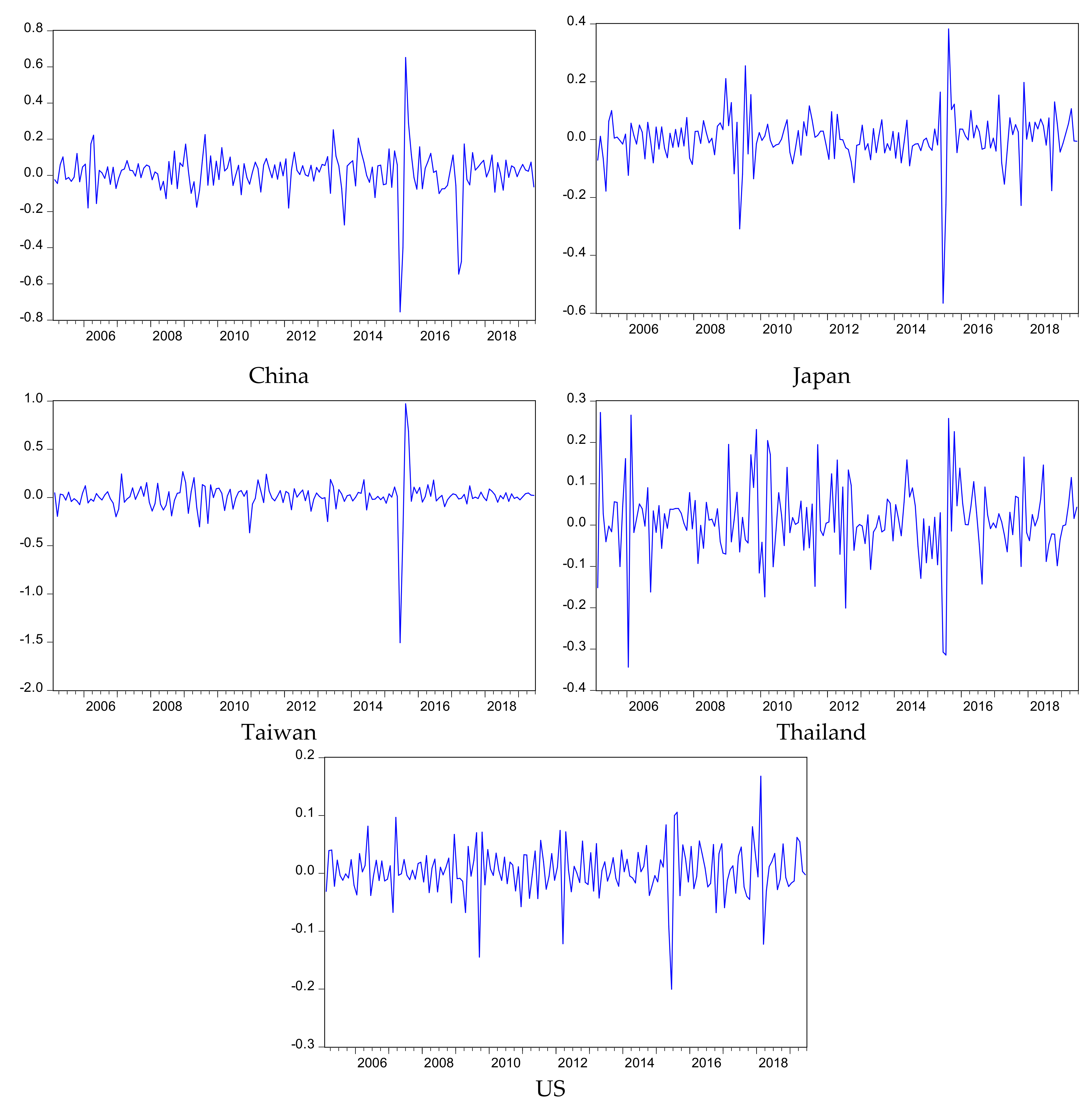
Figure 1 shows the volatility of tourist arrivals from five major markets to Korea. Most countries have significant fluctuations and show similar movements. All countries were affected by extreme events, such as the Middle East Respiratory Syndrome (MERS) outbreak in 2015, when tourist arrivals were drastically reduced. Additionally, tourist arrivals from China decreased sharply in March 2017 due to the THAAD issue. Table 2 reports the Pearson’s correlations between the change rates of tourist arrivals from the five countries.
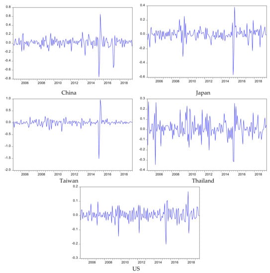
Figure 1.
Volatility of the tourist arrivals from five countries.

Table 2.
Pearson’s correlations.
Overall, the correlations are positive and are higher between China and Taiwan as well as between Japan and Taiwan than between the other pairs.
4. Results
4.1. Results for the Marginal Models
Table 3 presents the parameter estimates for the mean and variance equation of the AR (p)-GARCH (1, 1) model with a skewed Student’s t distribution for each country. The and of the mean equation are negative and highly significant for Taiwan and the US. According to the coefficients of variance equation, (short-run persistency) is positive and significant for China, Japan, and Thailand, which implies that a shock contributes to short-run persistence in these three countries. However, (long-run persistency) is positive and significant for all countries, indicating that a shock leads to long-run persistence in all countries. Comparing the effects of and , the results reveal that a short-run persistence of shocks is stronger than a long-run persistence of shocks in China, Japan, and Thailand, indicating a larger impact of short-run shocks on the tourism market volatility. Additionally, a coefficient of volatility persistence is referred to as (); the coefficients are 0.857 for China, 0.714 for Japan, 0.499 for Taiwan, 0.696 for Thailand, and 0.965 for the US, which indicates that volatility for the US is highly persistent regarding tourist arrivals when a shock occurs, while volatilities remain moderately persistent for China, Japan, and Taiwan, and lowly persistent for Thailand.

Table 3.
Result of the generalized autoregressive conditional heteroskedasticity (GARCH) (1,1).
4.2. Results of the Static and Time-Varying Copulas
We used various copulas to investigate the dependence structure and tail dependence for each pair of source countries. Table 4 reports the results of Kendall’s tau and the lower and upper tail dependences for the optimal copula model for each of the ten pairs. For the pairs of Japan–Taiwan, Japan–US, Taiwan–Thailand, Taiwan–US, and Thailand–US, the Student’s t copula is the best-fitting model. Additionally, the dependencies between China–Japan, China–Thailand, and Japan–Thailand are best explained by the Survival-Joe copula. The Gaussian is the best-fitting model for the pair of China–Taiwan, and the Survival-Gumbel copula is the best-fitting model for the pair of China–US.

Table 4.
Kendall’s tau and tail dependence of the best-fitting copula.
Kendall’s tau, which is transformed by the copula parameter, is used to compare the degree of correlation because each copula parameter value has a different range. Since Kendall’s tau correlation coefficient ranges from −1 to 1, it can evaluate the degree of linear and non-linear relationships. The Kendall’s tau of the optimal model shows positive values for all pairs, indicating there are interdependencies between the tourist arrivals of the five source countries and they tend to move together. Thus, as the number of tourist arrivals from one country increases (decreases), so does that from another country. However, the findings indicate that the strength of dependence between each pair of countries is relatively weak. Among them, the dependence strength of the China–Taiwan pair is the strongest, which is consistent with the fact that China and Taiwan share a similar culture and seasonal environment and tourist arrivals from the two countries to Korea have a strong interdependent relationship. In contrast, the dependence between Taiwan and Thailand is the weakest, suggesting there is little co-movement between tourist arrivals from Taiwan and Thailand to Korea. In particular, all countries paired with Thailand indicate a relatively low dependence, implying that tourist arrivals from Thailand to Korea are independent of those from the other four countries.
According to the coefficients of tail dependence in the optimal copula models, the pairs of Japan–Taiwan, Japan–US, Taiwan–Thailand, Taiwan–US, and Thailand–US have a symmetrical tail dependence, which indicates that markets move in the same direction for each of these pairs regardless of the type of shock (e.g., economic boom or recession, positive or negative extreme events). Conversely, the pairs of China–Japan, China–Thailand, China–US, and Japan–Thailand have a lower tail dependence, indicating tourist arrivals are likely to have higher dependence in the case of negative shocks than positive shocks. The highest value of tail dependence is 0.257 in the Japan–Thailand pair, suggesting that the co-movement between Japan and Thailand becomes stronger in negative extreme events. However, there is no tail dependence between China and Taiwan, indicating that the tourist arrivals from China and Taiwan are not highly correlated in extreme events. Overall, co-movement varies depending on the pair countries and type of shock, i.e., positive or negative.
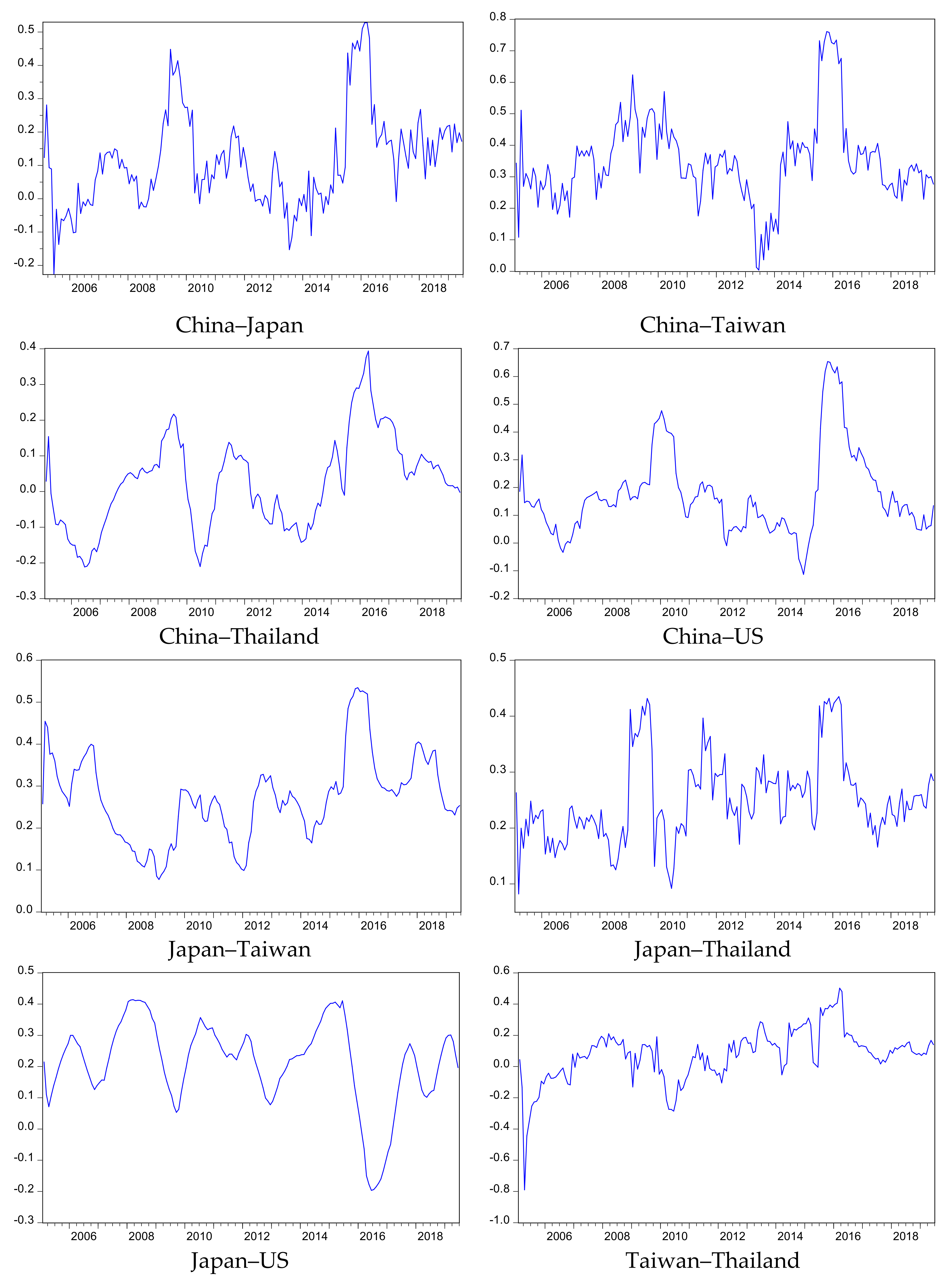
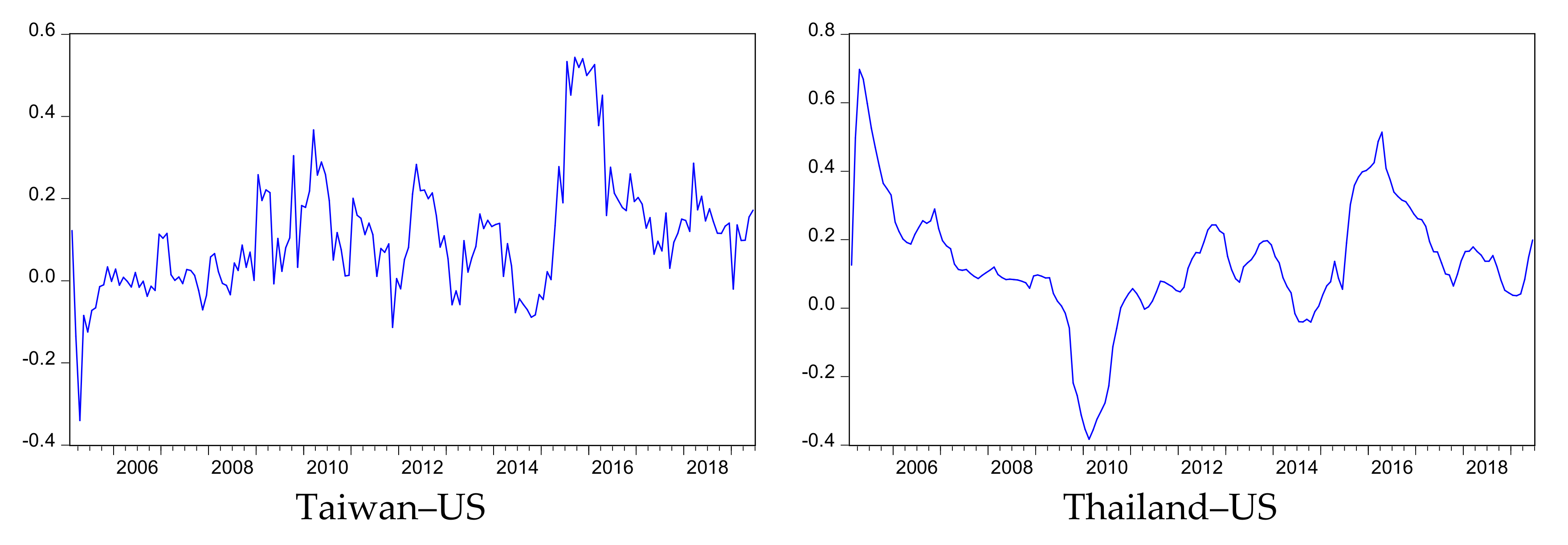
The dependence structure varies over time. Thus, we used the time-varying copula to identify co-movement between tourist flows from each pair of countries over the 15-year period. As shown in Figure 2, we find that all pair countries have a different dependence over time. The dependencies between China–Taiwan, Japan–Taiwan, and Japan–Thailand are positive over time. However, the dependencies among the remaining pairs change positively or negatively over time. Especially, the dependence between China and Taiwan is the highest among all pairs and close to 0.8 at a certain time, which indicates highly correlated markets and is recognized as the “complement effect”. Moreover, we find that the dependencies of all pairs are commonly high during extreme events, such as the 2008 financial crisis and 2015 MERS.
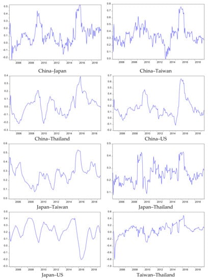
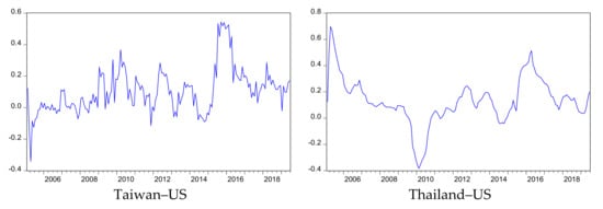
Figure 2.
The time-varying copula.
5. Conclusions
This study investigated the dependence among source countries of the inbound tourism market to Korea as well as tail dependence using static and dynamic copula models using secondary time series data, which consequently provides tourism policymakers with effective implications for the sustainability of the tourism industry.
Three main conclusions can be drawn from the results. First, estimates from the best-fitting copula models indicate dependencies among all inbound tourism market pairs, and the strongest market pair is interdependence between China and Taiwan.
Second, the extreme tail dependencies in tourist flow movements to Korea exist across the source countries. Four tourism market pairs (China–Japan, China–Thailand, China–US, and Japan–Thailand) move together in only negative shocks while five pairs (Japan–Taiwan, Japan–US, Taiwan–Thailand, Taiwan–US, and Thailand–US) show co-movements in both positive and negative conditions. Interestingly, the asymmetric extreme tail dependence between China and Taiwan does not exist even though the pairing has the highest static dependency.
Finally, co-movements for specific events can be identified through the dynamic dependence structure, and the result indicates that the China–Taiwan dependence is higher than the other time-varying structures, implying that Chinese and Taiwanese tourists to Korea complement each other. Based on the results, the destination managers and tourism policy maker could plan and design tourism events and attractions by investigating the characteristics, culture, and preferences (e.g., holidays, festivals) for inbound tourists from one country, and could develop marketing strategies for the inbound market for the other country. In this case, although China and Taiwan have a complementary relationship, tail dependence does not exist. The THAAD issue is one of the most extreme events affecting inbound tourism demand in Korea, which led to a decrease in the total tourist flows into Korea by 22.7% in 2017, due to a 48.3% reduction in Chinese tourists. During the same period, however, Taiwanese tourists increased by 11.1% [23]. This result highlights the importance of inbound tourism market substitutes to manage risks such as extreme events that are not a general worldwide or regional circumstance but occurs in relation to only one specific country. Therefore, other co-moving countries should be considered as respective substitutes for one another to form a highly complementary relationship. For example, although three markets, namely, Japan, Thailand, and the US, have extreme tail dependence on Taiwan in positive extreme events, the reliance on Japan rather than Thailand and the US markets is dominant, suggesting Japan as a substitute for China, and at the same time as a complement of Taiwan. The results imply that tourism policymakers should focus on developing tourism products/services to satisfy both Taiwanese and Japanese tourists. In addition, the results indicate it is important to substitute for the major inbound markets, since there are political and diplomatic relations with tourist source countries, in order for tourism destinations to generate stable revenue and maintain the sustainability of their tourism industry [2].
In future research, the static and dynamic dependencies between two-way tourist flows among market pairs need to be investigated because the overall circumstances of the markets, including neighboring or competing countries, should be considered [27]. The incorporation of two-way flows may lead to more accurate tourism demand forecasts.
Author Contributions
K.-H.C. and I.K. designed the research model, analyzed the data, and wrote the paper together. Both authors have read and agreed to the published version of the manuscript.
Funding
This research received no external funding.
Institutional Review Board Statement
Not applicable.
Informed Consent Statement
Not applicable.
Data Availability Statement
Data available on request.
Conflicts of Interest
The authors declare no conflict of interest.
References
- Puarattanaarunkorn, O.; Sriboonchitta, S. Copula based GARCH dependence model of Chinese and Korean tourist arrivals to Thailand: Implications for risk management. In Modeling Dependence in Econometrics; Springer: New York, NY, USA, 2014; pp. 343–365. [Google Scholar]
- Lean, H.H.; Smyth, R. Asian financial crisis, avian flu and terrorist threats: Are shocks to Malaysian tourist arrivals permanent or transitory? Asia Pac. J. Tour. Res. 2009, 14, 301–321. [Google Scholar] [CrossRef]
- UNWTO. UNWTO Tourism Highlights 2015 Edition; World Tourism Organization: Madrid, Spain, 2015; Available online: https://www.e-unwto.org/doi/pdf/10.18111/9789284416899 (accessed on 25 January 2021).
- Zeng, B.; Carter, R.W.; de Lacy, T. Short-term perturbations and tourism effects: The case of SARS in China. Curr. Issues Tour. 2005, 8, 306–322. [Google Scholar] [CrossRef]
- Cooper, M. Japanese tourism and the SARS epidemic of 2003. J. Travel Tour. Mark. 2005, 19, 117–131. [Google Scholar] [CrossRef]
- Ministry of Culture, Sport and Tourism. 2018 Nyeon-Gijun Gwangwang-Donghyangegwanhanyeoncha-Bogoseo (2018 Annual Report on Tourism Trends); Ministry of Culture, Sports and Tourism: Seoul, Korea, 2019.
- Henderson, J.C. The Great East Japan earthquake and tourism: A preliminary case study. Tour. Recreat. Res. 2013, 38, 93–98. [Google Scholar] [CrossRef]
- Pérez-Rodríguez, J.V.; Ledesma-Rodríguez, F.; Santana-Gallego, M. Testing dependence between GDP and tourism’s growth rates. Tour. Manag. 2015, 48, 268–282. [Google Scholar] [CrossRef]
- Conell, J.; Page, S.J.; Meyer, D. Visitor attractions and events: Responding to seasonality. Tour. Manag. 2015, 46, 283–298. [Google Scholar] [CrossRef]
- Getz, D. Event tourism: Definition, evolution, and research. Tour. Manag. 2008, 29, 403–428. [Google Scholar] [CrossRef]
- Sainaghi, R.; Baggio, R. Destination events, stability, and turning points of development. J. Travel Res. 2019, 1–12. [Google Scholar] [CrossRef]
- Chan, F.; Lim, C.; McAleer, M. Modelling multivariate international tourism demand and volatility. Tour. Manag. 2005, 26, 459–471. [Google Scholar] [CrossRef]
- Hoti, S.; McAleer, M.; Shareef, R. Modelling international tourism and country risk spillovers for Cyprus and Malta. Tour. Manag. 2007, 28, 1472–1484. [Google Scholar] [CrossRef]
- Seo, J.H.; Park, S.Y.; Yu, L. The analysis of the relationships of Korean outbound tourism demand: Jeju Island and three international destinations. Tour. Manag. 2009, 30, 530–543. [Google Scholar] [CrossRef] [PubMed]
- Shareef, R.; McAleer, M. Modelling the uncertainty in monthly international tourist arrivals to the Maldives. Tour. Manag. 2007, 28, 23–45. [Google Scholar] [CrossRef]
- Wang, K.; Chen, Y.-H.; Huang, S.-W. The dynamic dependence between the Chinese market and other international stock markets: A time-varying copula approach. Int. Rev. Econ. Financ. 2011, 20, 654–664. [Google Scholar] [CrossRef]
- Silva Filho, O.C.; Ziegelmann, F.A.; Dueker, M.J. Assessing dependence between financial market indexes using conditional time-varying copulas: Applications to Value at Risk (VaR). Quant. Financ. 2014, 14, 2155–2170. [Google Scholar] [CrossRef]
- Tang, J.; Sriboonchitta, S.; Ramos, V.; Wong, W.-K. Modelling dependence between tourism demand and exchange rate using the copula-based GARCH model. Curr. Issues Tour. 2016, 19, 876–894. [Google Scholar] [CrossRef]
- Tang, J.; Ramos, V.; Cang, S.; Sriboonchitta, S. An empirical study of inbound tourism demand in China: A copula-GARCH approach. J. Travel Tour. Mark. 2017, 34, 1235–1246. [Google Scholar] [CrossRef]
- Zhu, L.; Lim, C.; Xie, W.; Wu, Y. Modelling tourist flow association for tourism demand forecasting. Curr. Issues Tour. 2018, 21, 902–916. [Google Scholar] [CrossRef]
- Tang, J.; Sriboondita, S.; Yuan, X.; Wu, B. Volatility co-movement of China outbound tourism: Dynamic copula based GARCH model. Int. J. Innov. Manag. Inf. Prod. 2013, 4, 51–64. [Google Scholar]
- Juan, Y.; Choi, Y.; An, S.; Lee, C.-K.; Lee, S.J. The constraints of Chinese tourists to visit Korea caused by THAAD using Q-methodology. Asia Pac. J. Tour. Res. 2017, 22, 1261–1273. [Google Scholar] [CrossRef]
- Korea Tourism Knowledge and Information System Statistics on Tourists. Available online: http://tour.go.kr (accessed on 23 December 2019).
- Song, H.; Qiu, R.T.R.; Park, J. A review of research on tourism demand forecasting: Launching the annals of tourism research curated collection on tourism demand forecasting. Ann. Tour. Res. 2019, 75, 338–362. [Google Scholar] [CrossRef]
- Moore, W.R. The impact of climate change on Caribbean tourism demand. Curr. Issues Tour. 2010, 13, 495–505. [Google Scholar] [CrossRef]
- Peng, B.; Song, H.; Crouch, G.I. A meta-analysis of international tourism demand forecasting and implications for practice. Tour. Manag. 2014, 45, 181–193. [Google Scholar] [CrossRef]
- Song, H.; Li, G. Tourism demand modelling and forecasting—A review of recent research. Tour. Manag. 2008, 29, 203–220. [Google Scholar] [CrossRef]
- Akadiri, S.S.; Eluwole, K.K.; Akadiri, A.C.; Avci, T. Does causality between geopolitical risk, tourism and economic growth matter? Evidence from Turkey. J. Hosp. Tour. Manag. 2020, 43, 273–277. [Google Scholar] [CrossRef]
- Athanasopoulos, G.; de Silva, A. Multivariate exponential smoothing for forecasting tourist arrivals. J. Travel Res. 2012, 51, 640–652. [Google Scholar] [CrossRef]
- Coshall, J.T. A selection strategy for modelling UK tourism flows by air to European destinations. Tour. Econ. 2005, 11, 141–158. [Google Scholar] [CrossRef]
- Russell, R.; Faulkner, B. Entrepreneurship, chaos and the tourism area lifecycle. Ann. Tour. Res. 2004, 31, 556–579. [Google Scholar] [CrossRef]
- Mckercher, B. A chaos approach to tourism. Tour. Manag. 1999, 20, 425–434. [Google Scholar] [CrossRef]
- Sainaghi, R.; Baggio, R. Complexity traits and dynamics of tourism destinations. Tour. Manag. 2017, 63, 368–382. [Google Scholar] [CrossRef]
- Aloui, R.; Aïssa, M.S.B.; Nguyen, D.K. Conditional dependence structure between oil prices and exchange rates: A copula-GARCH approach. J. Int. Money Financ. 2013, 32, 719–738. [Google Scholar] [CrossRef]
- Hanif, W.; Hernandez, J.A.; Sadorsky, P.; Yoon, S.-M. Are the interdependence characteristics of the US and Canadian energy equity sectors nonlinear and asymmetric? North Am. J. Econ. Financ. 2020, 51, 101065. [Google Scholar] [CrossRef]
- Hanif, W.; Arreola-Hernandez, J.; Hussain Shahzad, S.J.; Hoang, T.H.V.; Yoon, S.-M. Regional and copula estimation effects on EU and US energy equity portfolios. Appl. Econ. 2020, 52, 5311–5342. [Google Scholar] [CrossRef]
- Kang, S.H.; Uddin, G.S.; Ahmed, A.; Yoon, S.-M. Multi-scale causality and extreme tail inter-dependence among housing prices. Econ. Model. 2018, 70, 301–309. [Google Scholar] [CrossRef]
- Wu, C.-C.; Chung, H.; Chang, Y.-H. The economic value of co-movement between oil price and exchange rate using copula-based GARCH models. Energy Econ. 2012, 34, 270–282. [Google Scholar] [CrossRef]
- Sklar, M. Fonctions de repartition and dimensions et leurs marges. Publications de l’ Institut de statistique de l’ Universite de Paris 1959, 8, 229–231. [Google Scholar]
- Bollerslev, T. Generalized autoregressive conditional heteroskedasticity. J. Econom. 1986, 31, 307–327. [Google Scholar] [CrossRef]
- Clayton, D.G. A model for association in bivariate life tables and its application in epidemiological studies of familial tendency in chronic disease incidence. Biometrika 1978, 65, 141–151. [Google Scholar] [CrossRef]
- Gumbel, E.J. Bivariate exponential distributions. J. Am. Stat. Assoc. 1960, 55, 698–707. [Google Scholar] [CrossRef]
- Joe, H. Parametric families of multivariate distributions with given margins. J. Multivar. Anal. 1993, 46, 262–282. [Google Scholar] [CrossRef]
- Joe, H.; Hu, T. Multivariate distributions from mixtures of max-infinitely divisible distributions. J. Multivar. Anal. 1996, 57, 240–265. [Google Scholar] [CrossRef]
- Cech, C. Copula-Based Top-Down Approaches in Financial Risk Aggregation. 2006. Available online: https://ssrn.com/abstract=953888 (accessed on 12 March 2020).
- Baum, T. Seasonality in tourism: Understanding the challenges: Introduction. Tour. Econ. 1999, 5, 5–8. [Google Scholar] [CrossRef]
- Baum, T.; Hagen, L. Responses to seasonality: The experiences of peripheral destinations. Int. J. Tour. Res. 1999, 1, 299–312. [Google Scholar] [CrossRef]
- Sainaghi, R.; Mauri, A.G.; Inanov, S.; d’Angella, F. Mega events and seasonality: The case of the Milan World Expo 2015. Int. J. Contemp. Hosp. Manag. 2019, 31, 61–86. [Google Scholar] [CrossRef]
Publisher’s Note: MDPI stays neutral with regard to jurisdictional claims in published maps and institutional affiliations. |
© 2021 by the authors. Licensee MDPI, Basel, Switzerland. This article is an open access article distributed under the terms and conditions of the Creative Commons Attribution (CC BY) license (http://creativecommons.org/licenses/by/4.0/).

