Examining the Driving Factors of the Direct Carbon Emissions of Households in the Ebinur Lake Basin Using the Extended STIRPAT Model

Abstract

In order to achieve the carbon emission reduction targets in Xinjiang, it has become a necessary condition to study the carbon emission of households in small and medium-sized cities in Xinjiang. This paper studies the direct carbon emissions of households (DCEH) in the Ebinur Lake Basin, and based on the extended STIRPAT model, using the 1987–2017 annual time series data of the Ebinur Lake Basin in Xinjiang to analyze the driving factors. The results indicate that DCEH in the Ebinur Lake Basin during the 31 years from 1987 to 2017 has generally increased and the energy structure of DCEH has undergone tremendous changes. The proportion of coal continues to decline, while the proportion of natural gas, gasoline and diesel is growing rapidly. The main positive driving factors affecting its carbon emissions are urbanization, vehicle ownership and GDP per capita, while the secondary driving factor is residents’ year-end savings. Population, carbon intensity and energy consumption structure have negative effects on carbon emissions, of which energy consumption structure is the main factor. In addition, there is an environmental Kuznets curve between DCEH and economic development, but it has not yet reached the inflection point.

1. Introduction

Since the industrial revolution, with the rapid development of the economic level of various countries, the world’s consumption of fossil fuels has continued to increase, resulting in the continuous increase in carbon dioxide and other greenhouse gas emissions. The 36th meeting of IPCC in 2013 reviewed and accepted the full report “Climate Change 2013. The Physical Science Basis”, which pointed out that the average temperature of the global land and ocean increased by 0.85 °C between 1880 and 2012, and the report indicated human activities is the main cause of global warming [1]. As an emerging market, China has become the world’s largest carbon emitter with a long-term growth model of high consumption and high pollution while simultaneously developing industrialization and urbanization. At present, China’s carbon emissions exceed that of the United States, and it has become the world’s second largest country in energy consumption and the largest country in greenhouse gas emissions [2].

Household consumption is an important source of greenhouse gas emissions. Household carbon emissions are divided into direct carbon emissions and indirect carbon emissions. About 20% of global greenhouse gas emissions came directly from household consumption, most of which came from fuel used for heating, cooling, cooking, illumination and private car [3]. Several studies have shown that household carbon emissions cannot be ignored [4,5]. In fact, it has become one of the main sources of carbon emissions in China [6].

In the past 20 years, a large number of scholars have conducted multiple studies on household carbon emissions. Kenny and Gray [7] used a model specifically designed for Ireland to calculate the carbon dioxide emissions of Irish households and the results show that the higher the occupancy rate, the more the energy efficiency of households. Weber and Perrels [8] used the input–output method to analyze the impact of household lifestyles in countries such as France, Germany, and the Netherlands on carbon emissions. Germany and the Netherlands have higher carbon emissions than France. Spangenberg and Lorek [9] used the ecological footprint method to analyze the carbon emissions from the energy consumed by households in the daily life, and the impact on the ecological environment. Song et al. [10] used an environmentally expanding multi-regional input-output model to analyze the carbon footprint of American households. The proportion of American households’ overseas carbon footprints continues to expand and the main sources of domestic carbon footprints in the United States are housing and transportation. Liu et al. [11] combined consumer lifestyle methods with input–output analysis to measure the indirect carbon emissions of Chinese urban households, and found that more than 58% of indirect carbon emissions came from 40% of high-income people. Hu et al. [12] came to an interesting conclusion that, in China, households with a large proportion of middle-aged and elderly people are beneficial to reducing household energy consumption. The conclusions of these studies are very meaningful and valuable. However, the country is a large research area, and the economic and environmental differences of provinces and regions within each country are huge, so many scholars have begun to conduct research on provincial units. Fan and Fang [13] breakdown the carbon emission factors of residents in Qinghai Province. The results show that household consumption level is the main factor, followed by carbon emission intensity and economic structure. Zeqiong et al. [14] studied the direct residential carbon emissions in Guangdong Province, the energy consumption structure and the urban and rural population structure have little impact, and the per capita consumption and population size have a significant impact.

The increase in global temperature has more obvious impacts on the ecological environment of arid regions. Elevated temperature has led to the increase in evaporation of rivers and lakes, and the transpiration of plants has become more intense, which has aggravated the contradiction between the supply and demand of water resources in arid regions, and the land desertification has become serious. In the process of humans and the natural environment competing for the few water resources, the ecological environment has been destroyed, triggering a variety of natural disasters, and damaging the quality of social and economic development. In order to better understand the environmental impact of household energy use, we have narrowed the research area. We selected the Ebinur Lake Basin (Figure 1) in the Xinjiang Uygur Autonomous Region as the research area. There have been many studies on carbon emissions in Xinjiang, but the research on carbon emissions in Xinjiang started relatively late, and the research areas involved are not large. Wang and Wang [15] research results show that in Xinjiang, per capita GDP growth is the most important driving force for the rapid growth of carbon emissions, and changes in the production structure have become a new main driving force for the rapid increase in carbon emissions. Gunther et al. [16] quantified the carbon footprint of cotton production in Xinjiang, and analyzed the spatial and temporal differences and driving factors of agricultural carbon emissions in Xinjiang. Zhou et al. [17] calculated the carbon emissions from thermal power industry in Xinjiang. Cui et al. [18] studied the spatial pattern of industrial carbon emissions in prefecture-level cities in Xinjiang. Although the research on DCEH is deepening, there are still some shortcomings. First of all, there are few studies on carbon emissions in Xinjiang on the whole, especially those involving DCEH. Secondly, there are great differences among different regions in Xinjiang, both in terms of DCEH itself and its influencing factors. The Ebinur Lake is the largest saltwater lake in Xinjiang, maintaining the ecological balance of the entire northern Xinjiang. However, it is a lake in an arid area with typical desert ecological environment, with sparse precipitation (89.80–169.70 mm) [19]. As for the Ebinur Lake Basin, because of the existence of abundant water resources and tourism resources, its agriculture and tourism are relatively developed. Compared with other regions in Xinjiang, the rural economy in the Ebinur Lake Basin is relatively developed. Due to tourism and agriculture, the DCEH in the rural areas of Ebinur Lake Basin is also greatly different. At present, the environmental problems of the Ebinur Lake Basin are very acute, facing serious problems such as lake shrinkage, water level decline, and rapid desertification. Therefore, the direct carbon emissions of households in the Ebinur Lake Basin can be calculated to understand its dynamic development trend and provide a benchmark for regional carbon neutral. The key direction of carbon emission reduction in the Ebinur Lake Basin can be identified by analyzing the impact of different factors in different periods. Moreover, the Ebinur Lake Basin not only has a large amount of fossil energy such as oil and natural gas, but also has abundant renewable energy, such as wind energy and solar energy [20]. Therefore, studying the direct household carbon emissions and driving factors in this area has practical operability and policy implementation.

2. Materials and Methods

2.1. The Calculation Method of DCEH

In this study, according to the administrative division of the Ebinur Lake Basin, the DCEH of the Ebinur Lake Basin is calculate. Calculated energy sources include raw coal, coke oven gas, other gas, gasoline, kerosene, diesel oil, liquefied petroleum gas, other petroleum products and natural gas. At this stage, some rural households in the Ebinur Lake Basin still use raw fuelwood for cooking and heating (2–10%) [21,22]. However, when government departments collect energy consumption data, fuelwood is not included. Therefore, the actual energy consumption of rural households will be higher than the results calculated in this paper.

CO₂ emissions are calculated according to IPCC guidelines, and carbon dioxide emissions related to fossil fuels can be calculated as energy consumption multiplied by emission factor, as follows:

$$C{E}_{energy}=\sum \sum C{E}_{ij}=\sum \sum E_{ij}\times LC{V}_i\times E{F}_i\times O_i$$

(1)

where CE_ij is carbon dioxide emissions from the burning of fossil fuel i in sector j, E_ij is fossil fuel consumption (10⁴ tons of standard coal equivalent, Mtce), LCV_i represents the lower calorific value of fuel I, EF_i represents the carbon dioxide emission factor of fuel i (the numerical value is equal to the fuel i carbon emission factor multiplied by 44/12, where 44/12 is the ratio of carbon dioxide to carbon molecular weight), and O_j represents the oxidation rate of fuel i. The combustion emission parameters of 9 fuels involved in this paper are from IPCC [23], National Development and Reform Commission [24], and [25,26] (

Table 1. The combustion emission parameters of fossil fuels.

Energy Types	LCV (MJ/t, Mm3)	CF (t ce/t, 103 m3)	Oxidation Rate	EF (t CO2/TJ)
Raw coal	20.9	0.714	0.94	96.51
Coke oven gas	16.1	0.593	0.94	78.8
Other gas	8.3	0.624	0.94	78.8
Gasoline	43.1	1.471	0.98	69.3
Kerosene	43.1	1.471	0.98	71.87
Diesel oil	42.7	1.457	0.98	74.07
Liquefied petroleum gas	50.2	1.714	0.98	63.07
Other petroleum products	43.0	1.429	0.98	74.07
Natural gas	38.9	1.330	0.99	56.17

)

2.2. STIRPAT Model

The IPAT model, which was proposed by Eheilich and Holden in the 1970s [27], shows that the three direct factors affecting the environment are population, wealth and technology, and the interaction. The equation is as follows:

$$I=P\times A\times T$$

(2)

In the model, I represents the environmental pressure, P is the population factor, A is affluence, and T is technology factor. The IPAT model reflects the relationship between the four factors while keeping other variables unchanged, and the coefficients between the factors are equal to 1, which is a conceptual description and is only suitable for qualitative research. There are some limitations in the application of this model. With the complexity of the study, its disadvantages have gradually emerged.

In order to overcome the limitations in research, two scholars, Dietz and Rosa, proposed the STIRPAT random model based on the IPAT model extension [28]

$$I=\beta P^a{A}^b{T}^c\mu$$

(3)

where $\beta$ is the model parameter, a, b and c are the index terms of population factors, affluence and technology level, and $\mu$ is the error term of the model. STIRPAT model has strong flexibility and can be extended according to the research content. Perform logarithm processing on Equation (3) to obtain Equation (4):

$$\ln I=\ln \beta +a\ln P+b\ln A+c\ln T+\ln \mu$$

(4)

Take ln I as the dependent variable, lnP, lnA and lnT as independent variables, lnβ as the constant term, and lnμ as the error term. According to the concept of elastic coefficient, when other influencing factors remain unchanged, each 1% change in driving force influencing factors (P, A, T) will cause I to change by a%, b%, and c%, respectively.

Based on the actual situation of the Ebinur Lake Basin, the population size and urbanization rate are selected as two variables of the population factor (P) to explore the impact of changes in population number and population structure on carbon emissions. Motor vehicle ownership (including agricultural machinery), GDP per capita and resident year-end savings are selected as three variables of affluence to represent the impact of affluence on carbon emissions. At the technical level, carbon intensity and energy consumption structure are introduced to study the impact of changes in energy consumption structure on carbon emissions. The specific variable interpretation is shown in

Table 2. Descriptive analysis of variables.

Variable	Definition Measuring Method	Unit
carbon emissions (I)	DCEH in the Ebinur Lake Basin	104 tons
Population size (P1)	Total population of Ebinur Lake Basin	104 people
Urbanization (P2)	Percentage of urban population in total population	%
Motor vehicle ownership (A1)	The number of motor vehicles in Ebinur Lake Basin	104 unit
GDP per capita (A2)	The ratio of GDP to total population	104 yuan
Resident year-end savings (A3)	The total amount of resident savings at various savings institutions at the end of each year	100 million yuan
Carbon intensity (T1)	The ratio of carbon emissions to GDP	t/104 yuan
Energy consumption structure (T2)	Percentage of coal consumption to total energy consumption	%

:

Based on the expansion of STIRPAT model, the above 7 variables are introduced into model (4). The specific model equation is obtained as follows:

$$\ln I=\ln \beta +a_1\ln P_1+a_2\ln P_2+b_1\ln A_1+b_2\ln A_2+b_3\ln A_3+c_1\ln T_1+c_2\ln T_2+\ln \mu$$

(5)

where lnβ represents constant term, lnμ represents error term. lnI is dependent variable, lnP_i, lnA_i and lnT_i are independent variables. a_i, b_i and c_i are elasticity coefficients of lnP_i, lnA_i and lnT_i, respectively.

2.3. Data Sources

The Ebinur Lake Basin includes Bortala Mongolian Autonomous Prefecture, Kuitun City, Usu City, Toli Country and Dushanzi District of Karamay. Due to the lack of statistical data in Dushanzi District, it is not available, so its energy consumption is not considered in the calculation. The economic and social development data of the above regions are from “Xinjiang 50 Years Data” [29], “Xinjiang Statistical Yearbook” [30], “Bortala Autonomous Prefecture Statistical Yearbook” [31], “Ili Kazakh Autonomous Prefecture Statistical Yearbook” [32] and their government bulletins. The data before 1987-2004 comes from “Xinjiang 50 Years Data “, which is a comprehensive statistical data set published at the 50th anniversary of the founding of Xinjiang. The data included is comprehensive and credible. The data after 2005–2017 comes from statistical yearbooks and government bulletins. The data of I is calculated in Equation (1).

The energy consumption for life from 1987 to 2004 comes from the “50 Years of Xinjiang”, and the energy consumption for life from 2005 to 2017 is calculated by the Energy Balance Sheet (EBT). EBT is a summary table that reveals the balance between the output, conversion and final consumption of energy in a region. It can reflect the form of energy balance and energy flow in a region. The consumption of fossil fuels in EBT can be used to calculate carbon emissions data related to fossil fuels. Xinjiang’s EBT is from the China Energy Statistics Yearbook [33]. However, most prefecture-level and county-level cities in China do not have EBT. Therefore, we derive the EBT of the city from the corresponding provincial energy balance sheet [26]; see Equations (3) and (4):

$$P=Inde{x}_{city}/Inde{x}_{province}\times 100\%$$

(6)

$$EB{T}_{city}=EB{T}_{province}\times P$$

(7)

Using the percentage of cities and provinces P, we narrow the provincial energy balance to the city level. For household consumption, we use population as an indicator.

2.4. Uncertainty and Monte Carlo Simulation

The collected data contain possible uncertainty caused by various reasons, e.g., the statistical estimation or human errors; therefore, estimating uncertainty is important for research [34]. As a method recommended by the IPCC, Monte Carlo simulations are widely used in the analysis of uncertainty [35], which is also employed in this study.

After repeating the simulation 10,000 times in Monte Carlo analysis, the average uncertainty of the data was calculated with a 95% confidence interval.

Table 3. Uncertainties of data.

Year	Sector	Lower Limit	Upper Limit	Sector	Lower Limit	Upper Limit
1997	I	−4.6%	10.5%	A2	1.4%	2.2%
	P1	2.0%	6.7%	A3	2.5%	7.6%
	P2	3.7%	8.1%	T1	−9.6%	8.3%
	A1	−1.7%	2.1%	T2	−1.4%	9.2%
2007	I	−3.3	11.7%	A2	−0.7%	1.1%
	P1	2.2%	6.3%	A3	4.8%	10.5%
	P2	1.5%	9.6%	T1	−5.4%	3.9%
	A1	−1.4%	3.5%	T2	−0.9%	8.4%
2017	I	−3.6%	8.0%	A2	0.3%	0.9%
	P1	0.1%	1.2%	A3	1.2%	6.7%
	P2	−0.6%	3.3%	T1	−7.1%	5.8%
	A1	−1.8%	2.1%	T2	0.9%	6.0%

shows the uncertainty of each type of data every 10 years. In general, A₂ has the smallest uncertainty, I has the greatest uncertainty. Since the Ebinur Lake Basin energy balance data is derived from provincial data, the potential uncertainty in the carbon emissions data may be higher. The credibility of the basic data is relatively high.

3. Analysis of Carbon Emissions and Energy Consumption Structure

3.1. Change in the Total Amount of DCEH

As shown in Figure 2, from 1987 to 2017, DCEH showed an overall growth trend, from 4.505 × 10⁵ t in 1987 to 1.922 × 10⁶ t in 2017, with an average annual growth rate of 5.2%. The proportion of DCEH by urban and rural households in Ebinur Lake Basin is shown in Figure 3. The proportion of direct carbon emissions of urban household consumption was the lowest in 1987, 36.82%, and the highest in 2004, 56.10%. From 1987 to 2014, although the proportion of urban areas fluctuated occasionally, the overall gap between urban and rural areas was narrowing, and the proportion of urban areas in some years even exceeded that of rural areas. The main reasons are as follows: (1) the growth rate of urban population exceeds that of rural population; (2) there are large numbers of rural people moving to cities; (3) urban household motor vehicle ownership is growing rapidly [36]. After 2014, the proportion of urban areas has gradually decreased, which is mainly due to the change of energy structure.

3.2. Analysis of Driving Factor

3.2.1. Population (P)

As shown in Figure 4, the total population of the Ebinur Lake Basin increased from 58.84 × 10⁴ in 1987 to 94.99 × 10⁴ in 2017, with an average annual growth rate of 1.67%. Generally speaking, it is growing steadily, but at a slow rate.

The level of urbanization increased slowly from 1987 to 2004, increasing by 8.1%.The urbanization fluctuations after 2008 were relatively large, indicating that the population flow speed was fast, and the household registration system began to be relaxed. In the next 10 years, the level of urbanization, however, has hardly changed, only increasing by 0.3%. By 2017, the level of urbanization fell back to 47.3%.

3.2.2. Affluence (A)

Figure 5 shows the change of the three factors in the level of Affluence (A) (1987–2017). The GDP per capita of the Ebinur Lake Basin increased from 1600 yuan in 1987 to 6.78 × 10⁴ yuan in 2017, an increase of about 42.4 times, with an average annual growth rate of 13.8%.

Economic development and urban expansion have rapidly increased the number of vehicles (agricultural machinery) that consume fossil fuels. Motor vehicles are an important contributor to carbon emissions, and the annual growth rate of carbon emissions in Xinjiang’s transportation industry exceeds 30% [37]. The number of motor vehicles in the Ebinur Lake Basin increased from 1.49 × 10⁴ in 1987 to 14.72 × 10⁴ in 2017, an increase of 9.88 times.

The year-end household savings in the Ebinur Lake Basin increased from 173.2 million yuan in 1987 to 17.08 billion yuan, an increase of 97.6 times, far exceeding the growth rate of GDP per capita. This not only shows that the residents of the Ebinur Lake Basin have a strong sense of saving money, on the other hand, it also suggests that the residents may be conservative in the consumption of living energy and have a strong carbon emission potential.

3.2.3. Technology (T)

As shown in Figure 6, The carbon intensity of the Ebinur Lake Basin decreased from 4.86 × 10⁴ yuan/ton in 1987 to 3 thousand yuan/ton in 2017, a 16.2 times reduction. The degree of reduction is higher than the degree of local development. There were certain fluctuations between 1995 and 1999. Although carbon intensity cannot fully reflect the level of energy efficiency, it suggests a certain extent that energy use during this period of development was extensive and the efficiency was extremely low. Generally speaking, the economic growth of the Ebinur Lake Basin has gradually reduced the driving force of carbon emissions.

Figure 6, Figure 7 and Figure 8 are used to show structural change in energy consumption of household. From 1987 to 2003, the energy consumption structure remained basically unchanged, and coal was in an absolute dominant position. After that, the share of coal began to decrease, down to 0.5–0.6. Since there was no detailed energy balance sheet before 2000, for the analysis of the detailed energy structure, the time span of the data we selected is from 2000 to 2017. Figure 7 and Figure 8 are the energy structure of direct carbon emissions from urban and rural households from 2000 to 2017, respectively. The energy structure of urban consumption has undergone tremendous changes. Raw coal and liquefied petroleum gas have been gradually replaced by natural gas. The consumption of raw coal has decreased year by year, from 89.6% in 2000 to 21.6% in 2015. Urban natural gas consumption increased year by year, from 0.4% in 2000 to 40.9% in 2014. Liquefied petroleum gas has experienced a process of increasing and decreasing, which indicates that it is rapidly eliminated after being used in a large number in energy structure conversion. The main reason for the above changes is that Xinjiang has implemented a large-scale “coal to gas” policy [38].

Almost all of the rural energy consumption before 2005 comes from coal. After 2005, the rural energy structure has become rich. However, the lowest proportion of coal is more than 85%. In winter, rural households rely heavily on coal and its derivatives, and large amounts of coal are used for heating, which directly leads to high environmental pollution, especially carbon dioxide emissions [39]. Some towns close to the city are gradually included in the urban planning, and some households have begun to use natural gas and liquefied petroleum gas, so the proportion of them has increased.

The proportion of gasoline consumption is also increasing year by year, from 3.8 to 24.8% in cities and from 0 to 6.4% in rural areas. This suggests that the living standards of families are constantly improving, and that private car ownership is continuing to increase. From 2011 to 2017, the consumption of gasoline in rural areas increased rapidly due to the increase in private cars and public transportation. Similarly, from 2011 to 2015, the proportion of diesel fuel consumption in rural areas increased very fast, mainly due to the large increase in agricultural machinery. In 2016 and 2017, the proportion of diesel energy consumption decreased. The possible reasons are as follows: (1) relocation of remote villages reduces the use of diesel vehicles [40]; (2) rural road optimization makes the growth rate of small gasoline cars and family motorcycles higher than that of diesel cars.

4. Results and Discussion of STIRPAT Model

4.1. Multicollinearity Analysis

Logarithmically process each variable and analyze the correlation of each variable. The results are shown in

Table 4. Pearson’s correlation test results.

	lnI	lnP1	lnP2	lnA1	lnA2	lnA3	lnT1	lnT2
LnI	1.000	0.939 **	0.843 **	0.997 **	0.971 **	0.947 **	−0.930 **	−0.896 **
LnP1		1.000	0.979 **	0.960 **	0.946 **	0.974 **	−0.946 **	−0.785 **
LnP2			1.000	0.934 **	0.942 **	0.960 **	−0.950 **	−0.794 **
LnA1				1.000	0.976 **	0.961 **	−0.943 **	−0.886 **
LnA2					1.000	0.980 **	−0.990 **	−0.903 **
LnA3						1.000	−0.982 **	−0.824 **
LnT1							1.000	0.868 **
LnT2								1.000

** Correlation was significant at the 0.01 level (2-tailed).

. There is a significant correlation between each factor and LnI, and there is a high correlation between variables, so there may be serious multicollinearity.

The logarithmic STIRPAT model is a typical multivariate linear equation. Therefore, in the process of model analysis, this article chose ordinary least squares (OLS). Intuitive judgment of multicollinearity is generally reflected by variance inflation factor (VIF). The larger VIF is, the more serious the collinearity is. When 0 < VIF < 10, there is no multicollinearity; when 10 ≤ VIF < 100, there is strong multicollinearity; when 100 ≤ VIF, there is serious multicollinearity. The analysis results are shown in

Table 5. OLS results.

	Unstandardized Coefficients	t Statistic	Sig.	VIF
C	4.135	2.471	0.021
LnP1	0.053	1.806	0.084	49.100
LnP2	0.076	0.852	0.403	11.725
LnA1	0.601	6.448	0.000	214.918
LnA2	0.086	1.314	0.202	217.306
LnA3	0.011	0.186	0.854	229.480
LnT1	−0.163	−0.403	0.691	173.467
LnT2	−0.026	−0.261	0.797	16.435
R2	0.998
adjusted R2	0.997
F statistic	1364.487
Sig.	0.000

. R² is 0.998, adjusted R² is 0.997, F statistic is 1347.370, and Sig is significant. All these indicate that there is a significant multivariate linear relationship between model factors. VIF values of all factors were greater than 10, the minimum LnT₂ was 11.725, and the maximum LnA₃ was 229.480, which further indicated that there was major multicollinearity among variables.

4.2. Principal Component Analysis

In order to solve the multicollinearity problem of the STIRPAT model, the principal component analysis method is used to combine multiple indicators into a few independent new variables that can fully reflect the overall information for further analysis. Principal component analysis is carried out on the variables mentioned above, and the results are shown in

Table 6. Total variance interpretation.

Indicators	Initial Eigenvalue			Extraction Sums of Squared Loadings
	Total	Variance	Cumulative%	Total	Variance	Cumulative%
1	6.574	93.911	93.911	6.574	93.911	93.911
2	0.287	4.100	98.011	0.287	4.100	98.011
3	0.070	0.994	99.005
4	0.052	0.736	99.741
5	0.011	0.155	99.896
6	0.007	0.100	99.996
7	0.000	0.004	100.000

.

It can be seen from Table 5 that the seven independent variables have been analyzed to extract two principal components, represented by Z₁ and Z₂. The two principal component variables can explain 98.011% of the original variable, indicating that Z₁ and Z₂ can well summarize the characteristics of the independent variable. According to the score coefficient of the principal component, the relationship between Z₁ and Z₂ and the original seven independent variables is:

$$Z_1=0.148\ln P_1+0.147\ln P_2+0.149\ln A_1+0.151\ln A_2+0.150\ln A_3-0.150\ln T_1-0.136\ln T_2$$

(8)

$$Z_2=0.686\ln P_1+0.628\ln P_2-0.109\ln A_1-0.197\ln A_2+0.386\ln A_3-0.033\ln T_1+1.555\ln T_2$$

(9)

Taking Z₁ and Z₂ as independent variables and lnI as the dependent variable, a regression model was established. The R² of the regression equation was 0.952, which passed the significance test at 0.01 level. The relationship between the principal component variables Z₁, Z₂ and lnI is as follows:

$$\ln I=0.930Z_1-0.208Z_2$$

(10)

Substitute Equations (8)–(10), calculate the logarithmic relation of STIRPAT model.

$$\ln I=-0.005\ln P_1+0.006\ln P_2+0.161\ln A_1+0.181\ln A_2+0.059\ln A_3-0.133\ln T_1+0.450\ln T_2$$

(11)

According to Equation (11), the main factors promoting carbon emission growth are motor vehicle ownership (A₁) and GDP per capita (A₂), while the secondary factor is residents’ year-end savings (A₃) and population urbanization (P₂). The reduction of carbon intensity (T₁) has a certain negative effect on the growth of carbon emissions, and energy consumption structure (T₂) has a strong negative effect on the growth of carbon emissions. The population size (P₁) has not become a positive factor for the growth of carbon emissions, but to a certain extent hindered the growth of carbon emissions.

4.3. Regression Analysis

The regression coefficient of population size (P₁) is negative, indicating that population growth has a negative effect on the growth of carbon emissions. The population of the Ebinur Lake Basin is not only small in size, but also grows very slowly, from 5.88 × 10⁵ in 1987 to 9.49 × 10⁵ in 2017. The average annual population growth rate is only 1.17%. The main reason is that the implementation of the family planning policy and the economic growth and education level have led to a decline in the family’s desire to have children [41]. Therefore, from this perspective, strict population policies and the development of education can curb the increase in carbon emissions. Studies by many scholars have shown that the impact of urbanization on carbon emissions is dynamic, and there are great differences in different regions [42,43]. Population urbanization (P₂) is a positive driver with a low degree of contribution from 1987 to 2017 in the results of this paper. Therefore, urbanization must be adapted to local conditions and cannot blindly pursue the transfer of population from rural to urban areas. Motor vehicle ownership (A₁), and GDP per capita (A₂) have a significant role in promoting the increase in DCEH. The fact that an increase in motor vehicle ownership (A₁) leads to an increase in carbon emissions is obvious and is consistent with the results [36,44,45]. Based on the regression results in this paper, there is an inverted U-shaped curve of the environmental Kuznets model between the GDP per capita (A₂) and the DCEH, but the inflection point has not yet been reached. In general, rapid urbanization is synergistic with the increase in carbon intensity, but with technological progress and economic growth, carbon intensity will gradually decline, leading to the gradual reduction of carbon emissions [5,46]. Due to the strong promotion of administrative forces in the Ebinur Lake Basin, the carbon intensity has been rapidly reduced, which is of great importance. In China, Xinjiang and other provinces, the energy consumption structure (T₂) is the main driving factor for the reduction of carbon emissions [47,48,49]. The energy structure has undergone tremendous changes and is the most important driving factor for reducing carbon emissions. Natural gas and liquefied petroleum gas is gradually replacing coal, so that carbon emissions are reduced when meeting the same needs of family life. However, in some developed regions, energy structure has become a secondary factor [14]. Therefore, the pressure on carbon emission reduction in the Ebinur Lake Basin is still huge.

5. Conclusions and Policy Recommendations

5.1. Conclusions

After several decades of urbanization and industrialization, China’s household income and consumption have been greatly developed, and the resulting carbon emissions have also increased several times. As one of the energy bases, Xinjiang Ebinur Lake Basin has unique customs and family living habits. In order to achieve its carbon emission reduction goals, it is necessary to breakdown the driving factors of its DCEH. Based on the extended STIRPAT model, the paper uses multiple linear analysis and principal component analysis to reveal the trends and causes of DCEH in the Ebinur Lake Basin from 1987 to 2017. The main conclusions are as follows:

(1)

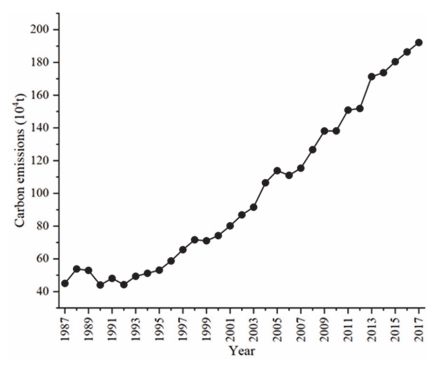
From 1987 to 2017, the DCEH in the Ebinur Lake Basin suggested an overall upward trend in growth. In most years, the proportion of rural consumption is higher than that of urban consumption. On the whole, the carbon emission potential and carbon emission reduction pressure of the Ebinur Lake Basin is great, and carbon emission will continue to increase;

(2)

From 2000 to 2017, the urban energy carbon emission structure changed greatly. Due to changes in energy policies, raw coal and liquefied petroleum gas were gradually replaced by natural gas. The rural energy structure has not changed much, and coal has always occupied an advantageous position. With the economic development, the increase in the number of motor vehicles has caused a huge change in the urban energy structure, and it has also enriched the rural energy structure;

(3)

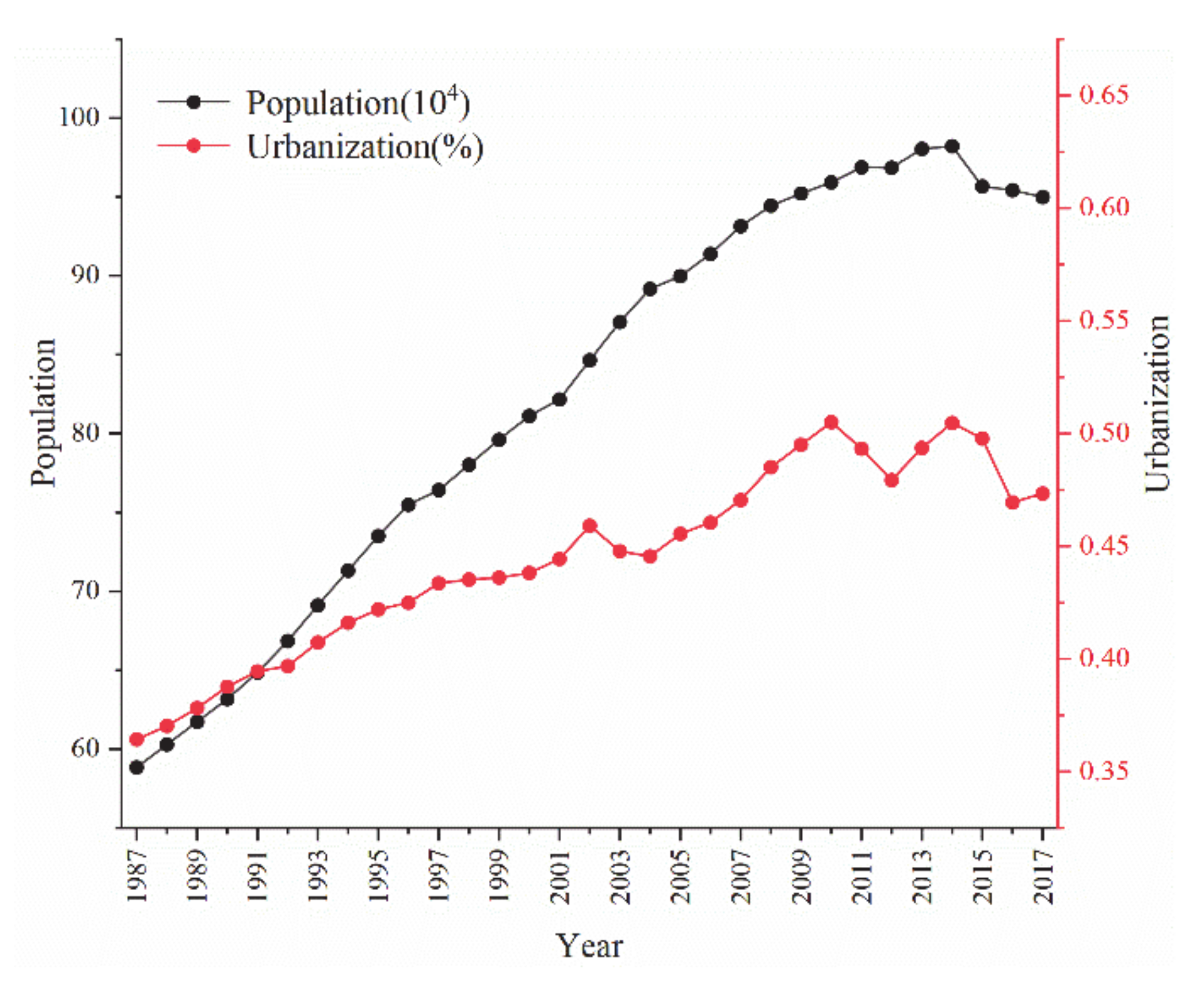
There is a significant affluence effect on the DCEH in the Ebinur Lake Basin. Motor vehicle ownership, GDP per capita, and residents’ year-end savings all play a positive role in carbon emissions. The population of the Ebinur Lake Basin has been growing at a slow rate, which has a slight negative effect on DCEH. The change in the structure of energy consumption is the main driver. In addition, there is an environmental Kuznets curve between DCEH and economic growth, but the inflection point has not yet been reached.

5.2. Policy Recommendations

(1)

Xinjiang’s renewable energy, especially wind energy and solar energy, is very rich. Increasing the proportion of renewable energy in total energy consumption can effectively optimize the energy consumption structure and has a significant positive effect on carbon dioxide emissions [50]. Local governments should further promote the use of clean energy and renewable energy, especially solar energy in family life;

(2)

The use of fossil fuels should be changed from high-carbon coal to relatively low-carbon petroleum, natural gas, and liquefied petroleum gas. At present, the heating, cooking and other activities of rural households in the Ebinur Lake Basin are still dominated by coal. In the reform process, it is necessary to fully consider that Xinjiang’s energy consumption structure is still dominated by coal, and it is necessary to continue to reduce the proportion of coal used in domestic energy consumption and improve the quality of coal used in rural areas; to accelerate the integration of rural areas around the city into the overall urban planning, optimize the quality and progress of urbanization so that natural gas and liquefied petroleum gas will gradually replace the niche occupied by coal in domestic energy;

(3)

The central and local governments should vigorously support and promote new energy vehicles (electric vehicles) and encourage and develop the new energy vehicle industry. The use of new energy vehicles in the Ebinur Lake Basin and even Xinjiang is not common, so it has broad application and promotion prospects. Public transportation and private cars in the urban area can gradually transition to new energy vehicles, which has both economic and environmental benefits.

References

1. Stocker, T.F.; Qin, D.; Plattner, G.-K.; Tignor, M.; Allen, S.K.; Boschung, J.; Nauels, A.; Xia, Y.; Bex, V.; Midgley, P.M.; et al. Climate Change 2013: The Physical Science Basis; IPCC: Geneve, Switzerland, 2013. [Google Scholar]
2. Liu, D.; Xiao, B. Can China achieve its carbon emission peaking? A scenario analysis based on STIRPAT and system dynamics model. Ecol. Indic. 2018, 93, 647–657. [Google Scholar] [CrossRef]
3. Ivanova, D.; Stadler, K.; Steen-Olsen, K.; Wood, R.; Vita, G.; Tukker, A.; Hertwich, E.G. Environmental Impact Assessment of Household Consumption. J. Ind. Ecol. 2016, 20, 526–536. [Google Scholar] [CrossRef]
4. Nejat, P.; Jomehzadeh, F.; Taheri, M.M.; Gohari, M.; Majid, M.Z.A. A global review of energy consumption, CO2 emissions and policy in the residential sector (with an overview of the top ten CO2 emitting countries). Renew. Sustain. Energy Rev. 2015, 43, 843–862. [Google Scholar] [CrossRef]
5. Dhakal, S. Urban energy use and carbon emissions from cities in China and policy implications. Energy Policy 2009, 37, 4208–4219. [Google Scholar] [CrossRef]
6. Zhu, Q.; Peng, X.; Wu, K. Calculation and decomposition of indirect carbon emissions from residential consumption in China based on the input–output model. Energy Policy 2012, 48, 618–626. [Google Scholar] [CrossRef]
7. Kenny, T.; Gray, N.F. A preliminary survey of household and personal carbon dioxide emissions in Ireland. Environ. Int. 2009, 35, 259–272. [Google Scholar] [CrossRef]
8. Weber, C.; Perrels, A. Modelling lifestyle effects on energy demand and related emissions. Energy Policy 2000, 28, 549–566. [Google Scholar] [CrossRef]
9. Spangenberg, J.H.; Lorek, S. Environmentally sustainable household consumption: From aggregate environmental pressures to priority fields of action. Ecol. Econ. 2002, 43, 127–140. [Google Scholar] [CrossRef]
10. Song, K.; Qu, S.; Taiebat, M.; Liang, S.; Xu, M. Scale, distribution and variations of global greenhouse gas emissions driven by U.S. households. Environ. Int. 2019, 133, 105137. [Google Scholar] [CrossRef]
11. Liu, X.; Wang, X.; Song, J.; Wang, H.; Wang, S. Indirect carbon emissions of urban households in China: Patterns, determinants and inequality. J. Clean. Prod. 2019, 241, 118335. [Google Scholar] [CrossRef]
12. Hu, Z.; Wang, M.; Cheng, Z.; Yang, Z. Impact of marginal and intergenerational effects on carbon emissions from household energy consumption in China. J. Clean. Prod. 2020, 273, 123022. [Google Scholar] [CrossRef]
13. Fan, Y.; Fang, C. Insight into carbon emissions related to residential consumption in Tibetan Plateau—Case study of Qinghai. Sustain. Cities Soc. 2020, 61, 102310. [Google Scholar] [CrossRef]
14. Zeqiong, X.; Xuenong, G.; Wenhui, Y.; Jundong, F.; Zongbin, J. Decomposition and prediction of direct residential carbon emission indicators in Guangdong Province of China. Ecol. Indic. 2020, 115, 106344. [Google Scholar] [CrossRef]
15. Wang, C.; Wang, F. Structural Decomposition Analysis of Carbon Emissions and Policy Recommendations for Energy Sustainability in Xinjiang. Sustainability 2015, 7, 7548–7567. [Google Scholar] [CrossRef] [Green Version]
16. Günther, J.; Thevs, N.; Gusovius, H.-J.; Sigmund, I.; Brückner, T.; Beckmann, V.; Abdusalik, N. Carbon and phosphorus footprint of the cotton production in Xinjiang, China, in comparison to an alternative fibre (Apocynum) from Central Asia. J. Clean. Prod. 2017, 148, 490–497. [Google Scholar] [CrossRef]
17. Zhou, X.; Zhou, M.; Zhang, M. Contrastive analyses of the influence factors of interprovincial carbon emission induced by industry energy in China. Nat. Hazards 2016, 81, 1405–1433. [Google Scholar] [CrossRef]
18. Cui, C.; Shan, Y.; Liu, J.; Yu, X.; Wang, H.; Wang, Z. CO2 emissions and their spatial patterns of Xinjiang cities in China. Appl. Energy 2019, 252, 113473. [Google Scholar] [CrossRef]
19. Ma, L.; Wu, J.; Liu, W.; Abuduwaili, J. Distinguishing between anthropogenic and climatic impacts on lake size: A modeling approach using data from Ebinur Lake in arid northwest China. J. Limnol. 2014, 73, 350–357. [Google Scholar] [CrossRef] [Green Version]
20. Fan, X.-C.; Wang, W.-Q.; Shi, R.-J.; Cheng, Z.-J. Hybrid pluripotent coupling system with wind and photovoltaic-hydrogen energy storage and the coal chemical industry in Hami, Xinjiang. Renew. Sustain. Energy Rev. 2017, 72, 950–960. [Google Scholar] [CrossRef]
21. Yun, X.; Shen, G.; Shen, H.; Meng, W.; Chen, Y.; Xu, H.; Ren, Y.; Zhong, Q.; Du, W.; Ma, J.-M.; et al. Residential solid fuel emissions contribute significantly to air pollution and associated health impacts in China. Sci. Adv. 2020, 6, eaba7621. [Google Scholar] [CrossRef]
22. Wang, Z. The Analysis of the Rural Household Energy Consumption in China; Harbin Institute of Technology: Harbin, China, 2018. [Google Scholar]
23. IPCC. IPCC Guidelines for National Greenhouse Gas Inventories; Institute for Global Environmental Strategies: Hayama, Japan, 2006. [Google Scholar]
24. NDRC. Guidelines for Provincal Greenhouse Gas Inventories; NDRC: Beijing, China, 2011. [Google Scholar]
25. Wang, C.; Zhang, X.; Wang, F.; Lei, J.; Zhang, L. Decomposition of energy-related carbon emissions in Xinjiang and relative mitigation policy recommendations. Front. Earth Sci. 2014, 9, 65–76. [Google Scholar] [CrossRef]
26. Shan, Y.; Guan, D.; Liu, J.; Mi, Z.; Liu, Z.; Liu, J.; Schroeder, H.; Cai, B.; Chen, Y.; Shao, S.; et al. Methodology and applications of city level CO 2 emission accounts in China. J. Clean. Prod. 2017, 161, 1215–1225. [Google Scholar] [CrossRef] [Green Version]
27. Holdren, J.P.; Ehrlich, P.R. Human Population and the Global Environment: Population growth, rising per capita material consumption, and disruptive technologies have made civilization a global ecological force. Am. Sci. 1974, 62, 282–292. [Google Scholar] [PubMed]
28. Dietz, T.; Rosa, E.A. Rethinking the Environmental Impacts of Population, Affluence and Technology. Hum. Ecol. Rev. 1994, 1, 277–300. [Google Scholar]
29. Qiu, Y. Xinjiang 50 Years Data, The Office of the Preparatory Committee for the 50th Anniversary of the Establishment of Xinjiang Uygur Autonomous Region; Bureau of Statistics of Xinjiang Uygur Autonomous Region, Ed.; China Statistics Press: Urumqi, China, 2005. [Google Scholar]
30. National Statistics Bureau of Xinjiang. Xinjiang Statistical Yearbook; China Statistics Press: Urumqi, China, 2018. [Google Scholar]
31. National Statistics Bureau of Bortala. Bortala Autonomous Prefecture Statistical Yearbook; China Statistics Press: Urumqi, China, 2018. [Google Scholar]
32. NBIL. Ili Kazakh Autonomous Prefecture Statistical Yearbook; China Statistics Press: Urumqi, China, 2018. [Google Scholar]
33. National Bureau of Statistics. China Energy Statistics Yearbook; China Statistics Press: Beijing, China, 2018. [Google Scholar]
34. Zheng, H.; Shan, Y.; Mi, Z.; Meng, J.; Ou, J.; Schroeder, H.; Guan, D. How modifications of China’s energy data affect carbon mitigation targets. Energy Policy 2018, 116, 337–343. [Google Scholar] [CrossRef] [Green Version]
35. Lang, J.; Cheng, S.; Zhou, Y.; Zhang, Y.; Wang, G. Air pollutant emissions from on-road vehicles in China, 1999–2011. Sci. Total Environ. 2014, 496, 1–10. [Google Scholar] [CrossRef]
36. Dong, J.-F.; Deng, C.; Li, R.; Huang, J. Moving Low-Carbon Transportation in Xinjiang: Evidence from STIRPAT and Rigid Regression Models. Sustainability 2017, 9, 24. [Google Scholar] [CrossRef] [Green Version]
37. Wang, X. Sustainable Development of Industry, Energy and Environment in Xinjiang Based on Carbon Footprint; Xinjiang University: Urumchi, China, 2017. [Google Scholar]
38. Sun, H.; Zhao, Z.; San, L. The development trend of China’s natural gas industry in 2013 and the outlook for 2014. Int. Pet. Econ. 2014, 22, 51–56. (In Chinese) [Google Scholar]
39. Maraseni, T.N.; Qu, J.; Yue, B.; Zeng, J.; Maroulis, J. Dynamism of household carbon emissions (HCEs) from rural and urban regions of northern and southern China. Environ. Sci. Pollut. Res. 2016, 23, 20553–20566. [Google Scholar] [CrossRef]
40. Xiong, C.; Yang, D.; Huo, J.; Zhao, Y. The Relationship between Agricultural Carbon Emissions and Agricultural Economic Growth and Policy Recommendations of a Low-carbon Agriculture Economy. Pol. J. Environ. Stud. 2016, 25, 2187–2195. [Google Scholar] [CrossRef]
41. Zhang, L.; Lei, J.; Zhou, X.; Zhang, X.; Dong, W.; Yang, Y. Changes in carbon dioxide emissions and LMDI-based impact factor decomposition: The Xinjiang Uygur autonomous region as a case. J. Arid Land 2013, 6, 145–155. [Google Scholar] [CrossRef] [Green Version]
42. Fang, Z.; Gao, X.; Sun, C. Do financial development, urbanization and trade affect environmental quality? Evidence from China. J. Clean. Prod. 2020, 259, 120892. [Google Scholar] [CrossRef]
43. Sun, W.; Huang, C.C. How does urbanization affect carbon emission efficiency? Evidence from China. J. Clean. Prod. 2020, 272, 122828. [Google Scholar] [CrossRef]
44. Yuan, R.-Q.; Tao, X.; Yang, X.-L. CO2 emission of urban passenger transportation in China from 2000 to 2014. Adv. Clim. Chang. Res. 2019, 10, 59–67. [Google Scholar] [CrossRef]
45. Ye, B.; Jiang, J.; Li, C.; Miao, L.; Tang, J. Quantification and driving force analysis of provincial-level carbon emissions in China. Appl. Energy 2017, 198, 223–238. [Google Scholar] [CrossRef]
46. Wang, F.; Wang, G.; Liu, J.; Chen, H. How does urbanization affect carbon emission intensity under a hierarchical nesting structure? Empirical research on the China Yangtze River Delta urban agglomeration. Environ. Sci. Pollut. Res. 2019, 26, 31770–31785. [Google Scholar] [CrossRef]
47. Wang, C.; Wang, F.; Zhang, X.; Yang, Y.; Su, Y.; Ye, Y.; Zhang, H. Examining the driving factors of energy related carbon emissions using the extended STIRPAT model based on IPAT identity in Xinjiang. Renew. Sustain. Energy Rev. 2017, 67, 51–61. [Google Scholar] [CrossRef]
48. Minx, J.C.; Baiocchi, G.; Peters, G.P.; Weber, C.L.; Guan, D.; Hubacek, K. A “carbonizing dragon”: China’s fast growing CO2 emissions revisited. Environ. Sci. Technol. 2011, 45, 9144–9153. [Google Scholar] [CrossRef]
49. Geng, Y.; Zhao, H.; Liu, Z.; Xue, B.; Fujita, T.; Xi, F. Exploring driving factors of energy-related CO2 emissions in Chinese provinces: A case of Liaoning. Energy Policy 2013, 60, 820–826. [Google Scholar] [CrossRef]
50. Paramati, S.R.; Sinha, A.; Dogan, E. The significance of renewable energy use for economic output and environmental protection: Evidence from the Next 11 developing economies. Environ. Sci. Pollut. Res. Int. 2017, 24, 13546–13560. [Google Scholar] [CrossRef]
Figure 1. The Ebinur Lake Basin administrative region
Sustainability 13 01339 g001
Figure 2. Direct carbon emissions of household from 1987 to 2017.
Sustainability 13 01339 g002
Figure 3. The ratio of DCEH from urban and rural households in the Ebinur Lake Basin from 1987 to 2017.
Sustainability 13 01339 g003
Figure 4. The change of Population (P) from 1987 to 2017.
Sustainability 13 01339 g004
Figure 5. The change of Affluence (A) from 1987 to 2017
Sustainability 13 01339 g005
Figure 6. The change of technology (T) 1987 to 2017.
Sustainability 13 01339 g006
Figure 7. Urban DCEH to the energy structure in the Ebinur Lake Basin from 2000 to 2017.
Sustainability 13 01339 g007
Figure 8. Rural DCEH to the energy structure in the Ebinur Lake Basin from 2000 to 2017.
Sustainability 13 01339 g008