A Hybrid Teaching-Learning-Based Optimization Algorithm for the Travel Route Optimization Problem alongside the Urban Railway Line

Abstract

Accurate travel route optimization is essential to promote and grow tourism in modern society. This paper investigates a travel route optimization problem alongside the urban railway line and proposes a hybrid teaching–learning-based optimization (HTLBO) algorithm. First, a mathematical programming model is established to minimize the total traveling time, in which the routes between and in different cities have to be appropriately determined. Then, a hybrid metaheuristic named HTLBO is proposed for solution generation. In HTLBO, depth first search (DFS) is utilized to obtain the optimal routes of any two stations in railway network, and a three-level coding method is designed to accommodate the problem characteristic. Besides, opposition-based learning (OBL) is embedded into teaching-learning-based optimization (TLBO) for enhancing HTLBO’s exploration ability, while variable neighborhood descent (VND) is used to enhance the algorithm’s exploitation ability. Finally, a case study is presented and simulation results verify HTLBO’s feasibility and effectiveness.

1. Introduction

With the rapid development of social economy, the people’s living standards have been significantly improved in China. Tourism is now becoming an essential part of peoples’ daily life [1,2]. In such contexts, scientific planning of travel routes is necessary to reduce traffic time and to improve tourist satisfaction [3]. This study is motivated by this background and aims to deal with a travel route optimization problem alongside the urban railway line.

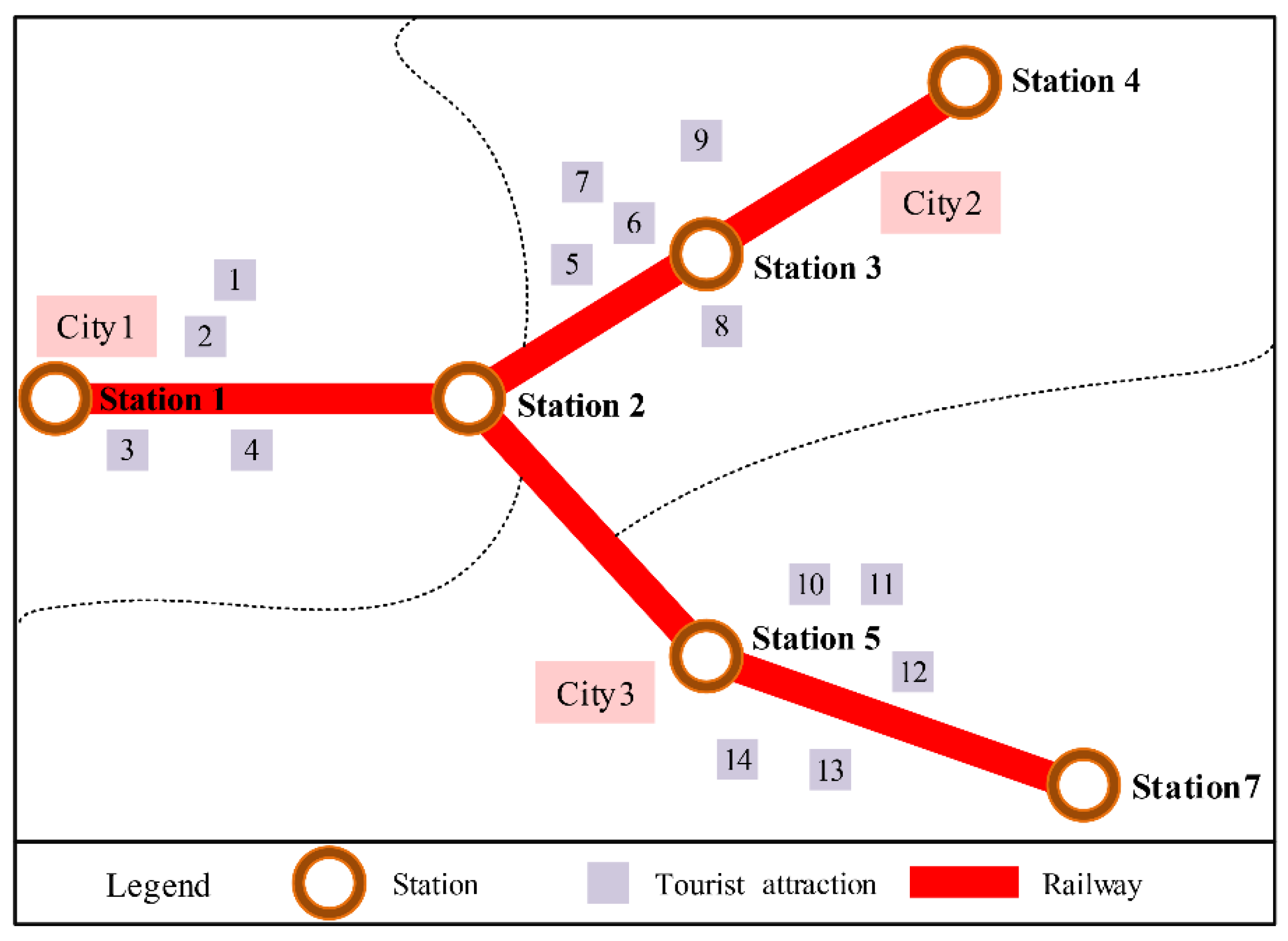
As mentioned above, this study investigated an optimization problem in which the total traveling time has to be minimized. Theoretically, the considered problem can be regarded as a variant of the classic travel salesman problem (TSP) [4], and Figure 1 presents a schematic diagram. In the specific problem setting, a traveler is planning to visit all tourist attractions in a set of cities. The way he travels between different cities is via the railway, and the railway network associated with these cities is predefined. For the considered problem, decisions should be made are described as follows: (1) the visiting sequence of different cities, (2) the railway route between different cities, and (3) the traveling routes in each city.

For the considered problem, the inherent complexity of the combinatorial optimization problem and the coupling of different subproblems make it difficult to obtain a satisfactory solution [5]. Besides, the specific constraints associated with practical applications further increase its difficulty. Therefore, this research is motivated in this context and focuses on designing an efficient decision-making method for solution generation.

A great many algorithms have been designed and introduced to solve travel route optimization problems, which can be divided into three categories: exact algorithms, heuristic methods, and metaheuristic algorithms [6]. Exact algorithms include dynamic programming, branch and bound algorithms, among others. These algorithms are capable of solve small-scale instances optimally. However, the computation time increases sharply with the increasing of instance size, which makes it impossible to solve medium and large-scale instance in reasonable time [7,8,9]. Heuristic methods were applied to solve different optimization problems by virtue of some classical scheduling rules, and the efficiency is impressive [10,11]. Despite that, such applications have strict requirements on the problem’s structure setting, and the algorithms’ generality are very poor. Under such circumstances, metaheuristic approaches are now becoming the most appropriate tools since these algorithms are problem-agnostic and can be adjusted to coordinate the problem-specific information [12]. Some effective metaheuristics have been designed and applied for solution generation of similar problems, including Genetic Algorithm (GA), Particle swarm optimization (PSO), and others. [13,14]. Meanwhile, there is a theorem called no free lunch (NFL) that has proven that there is no approach is best suited to tackle all optimization problems [15]. In other words, the superior performance of a metaheuristic approach on one problem cannot guarantee similar performance on other optimization problems [16]. This theorem is the foundation of many researches works that allows researchers in different fields to adjust different algorithms for their problems or propose some new algorithms. This is also the motivation and foundation of our research work, in which a novel metaheuristic method name HTLBO is designed and applied to solve the considered travel route optimization problem.

TLBO is one of the most recent metaheuristics, which has been proven to precede other classics metaheuristics in some applications [17]. It is inspired by behaviors of a classroom and contains two phases: teacher and learner phases. TLBO-related approaches with better algorithm performance have already been proposed by a great many researchers [18,19,20,21,22]. For most recent research work, please refer to the book presented by Rao [23]. Nevertheless, there still exist some challenges when introducing TLBO for different optimization problems [24]. First, TLBO is initially proposed for continuous problems and thus requires some modifications when applied to discrete problems. Second, it tends to get trapped into local optima when solving real-world scale instances, which is now a common weakness of population-based metaheuristics. Thus, researchers in different fields attempt to design appropriate coding and decoding schemes when introducing TLBO to discrete problems as well as to strengthen algorithm’s exploitation ability. The current research does make efforts in these regards and presents a new TLBO version for the considered travel route optimization problem.

To our best knowledge, the current research work is the first attempt to develop a TLBO-version algorithm for the travel route optimization problem alongside the urban railway line. Four main contributions of this research work are summarized as follows:

• A mathematical model for the considered travel route optimization problem is formulated with an objective of minimizing the total traveling time.
• The HTLBO algorithm is proposed to solve considered problem by combining TLBO metaheuristic and DFS method.
• A new solution representation technique is designed to accommodate the problem characteristic.
• The OBL and VND techniques are embedded into HTLBO on purpose of enhancing algorithm’s performance.

The remainder of this work is organized as follows. Section 2 presents the problem description and the mathematical program model. Section 3 illustrates the theory of TLBO, and Section 4 establishes the proposed HTLBO by combing TLBO with some efficient techniques. Computational experiments are discussed in Section 5. Finally, conclusions and future researches are presented in Section 6.

2. Problem Formulation

2.1. Problem Description

In this paper, a traveler is assumed to visit all tourist attractions in a set of cities. The railway network associated with these cities is known with certainty, and decisions should be made are: (1) the visiting sequence of different cities, (2) the railway route between different cities, and (3) the traveling routes in each city. The objective to be optimized is the total traveling time. Some premises are stated as follows:

• The traveler is assumed to travel by railway between any two cities, while the roads account for the traveling inside a city.
• The time span of the railway network as well as the road network is predefined.
• Once the traveler starts to visit one city, it is assumed that he will reach the city through one of its’ railway stations, then go through all tourist attractions by a certain order and leave from one railway station.
• The initial and finale position of the travel is assumed to be at one railway station of then a city.

2.2. Mathematical Model

The relevant notations used for describing the considered problem are collected as follows:

Parameters
$C$	Set of cities, $c\in C$
$S^c$	Set of railway stations in city $c$
$T^c$	Set of tourist attractions in city $c$
$V^c$	$V^c=S^c\cup T^c$$V^c=S^c$, set of railway stations and tourist attractions in city $c$
$E^c$	$E^c=\{(i,j)|i,j\in V^c\}$, set of directed edges in city $c$
$G^c$	$G^c=(V^c,E^c)$, the directed network graph of city $c$
$t_{ij}^c$	Time span from position $i$ to $j$ in city $c$, where $i,j\in V^c$ and $(i,j)\in E^c$
$V^r$	$V^r={\displaystyle \underset{c\in C}{\cup }{S}^c}$, set of railway stations in all cities
$E^r$	$E^r=\{(i,j)|i,j\in V^r\}$, set of directed edges of railway network
$G^r$	$G^r=(V^r,E^r)$, the directed network graph of railway stations in all cities
$t_{ij}^r$	Time span from station $i$ to $j$, where $i,j\in V^r$ and $(i,j)\in E^r$
Decision variables
$x_{ij}^c$	$x_{ij}^c\in \{0,1\}$, if the traveler visits tourist attraction $j$ right after $i$ in city $c$, $x_{ij}^c=1$, otherwise $x_{ij}^c=0$
$y_{ij}^r$	$x_{ij}^c\in \{0,1\}$, if the traveler visits station $j$ right after station $i$, $x_{ij}^c=1$, otherwise $x_{ij}^c=0$

By virtue of above problem description and notation definitions, the considered travel route optimization problem can be modeled as follows:

$$\min Z={\displaystyle \sum _{c\in C}{\displaystyle \sum _{i\in V^c}{\displaystyle \sum _{j\in V^c}{x}_{ij}^c•}}}{t}_{ij}^c+{\displaystyle \sum _{i\in V^r}{\displaystyle \sum _{j\in V^r}{y}_{ij}^r•t_{ij}^r}}$$

(1)

$${\displaystyle \sum _{j\in V^c}{x}_{ij}^c}=1,i\in T^c,c\in C$$

(2)

$${\displaystyle \sum _{i\in V^c}{x}_{ij}^c}=1,j\in T^c,c\in C$$

(3)

$${\displaystyle \sum _{t\in S^c}{\displaystyle \sum _{j\in V^c}{x}_{ij}^c=1}},c\in C$$

(4)

$${\displaystyle \sum _{i\in V^c}{\displaystyle \sum _{j\in S^c}{x}_{ij}^c=1}},c\in C$$

(5)

$$x_{ij}^c\in \{0,1\},i\in V^c,j\in V^c,c\in C$$

(6)

$$y_{ij}^r\in \{0,1\},i\in V^r,j\in V^r$$

(7)

The objective is described in Equation (1), which aims to minimize the total traveling time between and in different cities. Constraints (2) and (3) indicate that each tourist attraction in one city can be visited exactly only one time. Constraints (4) and (5) indicates that travelers enter into and leave from each destination city only through one railway station. Constraints (6) and (7) are the value range constraints of all decision variables.

3. TLBO Algorithm

TLBO algorithm is established by simulating behaviors in a classroom. It uses a group of individual solutions to proceed to a satisfactory solution. The evolution of TLBO includes two parts: ‘Teacher Phase’ and ‘Learner Phase’ Figure 2 illustrates a schematic diagram of TLBO.

Details of some critical steps in TLBO are described as follows:

(1)

Initialization

Let $N$ represents the population size and $x_i=(x_{i1},\cdots ,x_{id},\cdots ,x_{iD})$ be the $i$-the solution vector in the current population ($i=1,2,\cdots ,N$). Individual $x_i$ is generated by taking the following equation:

$$x_{id}=x_{{}_{id}}^l+rand(0,1)•(x_{{}_{id}}^u-x_{{}_{id}}^l)$$

(8)

where $x_{id}$ represents the $d$-th value of the solution vector $x_i$ and $[x_d^l,x_d^u]$ is range of dimension $d$. Notation $\mathrm{rand}(0,1)$ represents a uniform random number from interval [0,1].

(2)

Teacher Phase

The mean position of the current population, noted as $x^m=(m_1,\cdots ,m_d,\cdots ,m_D)$, is calculated and then to be used for solution update. Besides, the best solution found so far by TLBO is denoted as the teacher individual $x^{teacher}$. Given a parent individual $x^{old}$, the neighborhood search in this stage is implemented as follows

$$x^{new}=x^{old}+rand(0,1)•(x^{teacher}-\mathrm{TF}•x^m)$$

(9)

where the teaching factor $TF\in \{1,2\}$. A greedy selection strategy is used to update the candidate solutions. In others words, the better solutions between $x^{new}$ and $x^{old}$ will be retained.

(3)

Learner Phase

In the so-called “Learner Phase”, TLBO update a solution by comparing the position difference between the candidate solution and a randomly selected solution in current population. Specifically, given an individual $x^{old}$, a random solution $x^{rand}$($x^{rand}\ne x^{old}$) is selected. Then, the neighborhood search in this stage is carried out by taking the following equation:

$$x^{new}={\{}_{x^{old}+rand(0,1)•(x^{old}-x^{rand}),otherwise}^{x^{old}+rand(0,1)•(x^{rand}-x^{old}),iff(x^r)<f(x^{old})}$$

(10)

where notation $f(\cdot )$ represents the objective function to be optimized. Similarly, the greedy selection strategy is also used to determine the offspring individual.

4. HTLBO Algorithm

4.1. DFS Technique

In the considered problem, the traveler plans to reach different cities by virtue of the railway network. In such a context, HTLBO algorithm uses DFS technique to determine the shortest route between any two stations. DFS is a kind of tree search method in nature. It starts at the root node and explores as far as possible along each branch before backtracking [25].

To better illustrate the search process of DFS, an example is presented here. Figure 3 presents the schematic diagram of a directed railway network, and Figure 4 provides the route search process from station 1 to station 5. The total number of routes is 7, and the shortest route is “Station 1 → Station 2 → Station 3 → Station 5”. The path length is 2.20. In addition,

Table 1. Shortest route information in the proposed directed railway network.

Starting Point	Target	Path	Shortest Distance
1	2	1→2	0.22
1	3	1→3	0.60
2	3	2→3	0.28
1	4	1→4	1.62
2	4	2→4	0.92
3	4	3→4	0.88
1	5	1→2→3→5	2.20
2	5	2→5	1.88
3	5	3→5	1.48
4	5	4→5	0.92

summarizes the shortest route and path length between any two stations in the current railway network.

4.2. Encoding and Decoding

As TLBO is initially designed for continuous problems, a new solution representation technique is designed to accommodate the problem characteristic and used for the algorithm deployment.

Some details associated with coding process are summarized as follows. Given city se $C$, tourist attractions set $T^c$ and railway stations set $S^c$ ($c\in C$), HTLBO adopts three layers of real number to represent a solution of the considered problem. The value range of each layer is set to [0,1]. The first layer is used to determine the traveling order of all cities and its encoding length is $\left|C\right|$. The second layer is used to determine the station index the traveler entering into and leaving from each city. The corresponding encoding length is $2\cdot \left|C\right|$. The third layer is used to determine the traveling order of all tourist attractions in each city and the code length is $\left|{\displaystyle {\cup }_{c\in C}{S}^c}\right|$.

The decoding process includes two parts: ranked-order value (ROV) and roulette wheel rules [26,27]. ROV rule is used to convert a real number array into an integer sequence. HTLBO adopt ROV rule to determine the traveling order of all cities, as well as the tourist attractions visiting sequence in each city (see Figure 5a). The roulette wheel rule is used to determine the station index when traveler entering into or leaving from a city (see Figure 5b). The implementation process of the above two rules are illustrated in Figure 5.

By virtue of above preparations, the decoding process of a solution array for the considered problem is summarized as follows: First, ROV rule is used to obtain the traveling order of all cities. Then, roulette wheel rule is utilized to determine the station index when entering into or leaving from a city. Finally, the ROV rule is used to obtain the visiting order of all the tourist attractions in each city.

To clearly explain the above process, a concrete example is present here.

Table 2. Information of a concrete instance.

City Index	Set of Tourist Attractions	Set of Railway Stations
1	1,2,3	1,2
2	4,5,6,7	3,4,5
3	8,9,10	6,7

provides the set of tourist attractions as well as the set of railway stations in each city. On this basis, the coding length of each layer is 3, 6, and 10, respectively. Given three levels of coding ((0.22, 0.50, 0.31), (0.81, 0.30, 0.12, 0.51, 0.71, 0.31), (0.22, 0.31, 0.50, 0.43, 0.51, 0.90, 0.35, 0.23, 0.01, 0.99)), Figure 6 presents the corresponding decoding process.

The interpretation of such a solution array is described as follow:

• First, the traveler will enter in city 1 via station 2, then visit tourist attractions 1→2→3, and finally leave from the current city from station 1.
• Secondly, the traveler will enter in city 3 via station 7, then visit tourist attractions 9→8→10, and finally leave from the current city from station 6.
• Finally, enter city 2 via station 3, the traversal sequence of tourist attractions is 7→4→5→6, and leave the current city from station 4.

4.3. OBL

OBL is a simple but efficient method to enhance algorithm’s performance in swarm computation [28]. In the design of HTLBO, OBL is often used to improve the quality of population in two different ways.

First, OBL is used to generate initial solutions with high qualities. Given population size $N$ and the $i$-the solution $x_i=(x_{i1},\cdots ,x_{id},\cdots ,x_{iD})$ ($i=1,2,\cdots ,N$) in the current population, the reverse solution array $x_i^o=(x_{i1}^o,\cdots ,x_{id}^o,\cdots ,x_{id}^o)$ of $x_i$ is calculated by:

$$x_{id}^o=x_d^l+x_d^u-x_{id}$$

(11)

where $d=1,2,\cdots ,D$, $D$ represents the problem dimension and interval $[x_d^l,x_d^u]$ is the value range of the $d$-the dimension decision variable. The initialization of HTLBO is implemented by taking the following steps:

Step 1.

Let $i\leftarrow 1$ and $d\leftarrow 1$, then go to Step 2.

Step 2.

If $i\le N$, then go to Step 3; otherwise, go to Step 7.

Step 3.

If $d\le D$ is satisfied, go to Step 4; otherwise, go to Step 5.

Step 4.

Let $x_{id}=x_{id}^l+\mathrm{rand}(0,1)\cdot (x_{id}^u-x_{id}^l)$ and $x_{id}^o=x_d^l+x_d^u-x_{id}$, respectively; then, go to Step 5.

Step 5.

Let $d\leftarrow d+1$, if $d>D$ holds, let $d\leftarrow 1$ and go to Step 6; otherwise, go to Step 3.

Step 6.

Let $i\leftarrow i+1$, and then go to Step 2.

Step 7.

Select $N$ best solutions among $\{x_1,\cdots ,x_N,x_i^o,\cdots ,x_N^o\}$ to form the initial population.

Second, OBL is employed to explore the search space when the new generated solution is not superior to the candidate one in “Teacher Phase” or “Learner Phase”. For the candidate solution, the reverse solution is defined as follows:

$$x_{id}^o={\{}_{rand(0,1)•({\tilde{x}}_d^l-{\tilde{x}}_d^u)-x_{id},otherwise}^{x_d^l+x_d^u-x_{id},ifrand(0,1)<0.5}$$

(12)

where $[{\tilde{x}}_d^l,{\tilde{x}}_d^u]$ is the dynamic boundary of the current population, i.e., ${\tilde{x}}_d^l=\min \{x_{id}|i=1,2,\cdots ,N\}$ and ${\tilde{x}}_d^u=\max \{x_{id}|i=1,2,\cdots ,N\}$. Notation $\mathrm{rand}(0,1)$ represents a random number in interval [0,1].

4.4. Local Search

To better adopt TLBO for the considered problem, a local search method based on VND is designed in this subsection [29]. Given an initial solution, VND is performed in a deterministic way and it explores the search space by virtue of different mutation operators. In HTLBO, Gaussian mutation (GM), swap, reversion and insertion operators utilize to generate mutant solution array of a candidate one [30,31]. Details of each mutation operator are summarized as follows:

• GM: given the $d$-the dimension of solution array (denoted as $x_{id}$), the update process is implemented according to probability $P_{GM}$. The mathematical equations are:

  $$x_{id}={\{}_{x_{id}otherwise}^{GM(x_{id},{\sigma }_d)ifrand(0,1)<P_{GM}}$$

  (13)

  $${\sigma }_d=\frac{x_{id}^u-x_{id}^l}{{\sigma }_{scale}}$$

  (14)

  where $GM(x_{id},\sigma )$ denotes Gaussian sampling with mean $x_{id}$ and variance ${\sigma }_d$. Notation ${\sigma }_d$ is calculated by range $[x_{id}^l,x_{id}^u]$ and the scaling factor ${\sigma }_{scale}$ is a scaling factor. According to some related studies, $P_{GM}$ is set to the reciprocal of the total length of the code and ${\sigma }_{scale}$ is set to 20.
• Swap: randomly select two positions in a candidate solution array, and exchange values on these two positions (see Figure 7a).
• Reversion: randomly select two positions in a candidate solution array, and reverse values between these two positions (see Figure 7b).
• Insertion: randomly select two positions in a candidate solution array, and insert the value on a position before the other position (see Figure 7c).

Gaussian mutation can be utilized to update each lay of the candidate solution array, while the other three operators are applied to update the first, as well as the third layer. Given a candidate solution array $x_i$, a random permutation (denoted as $<{\Omega }_1,{\Omega }_2,{\Omega }_3,{\Omega }_4>$) of above-mentioned four operators are first generated. With a predefined iteration number $L{S}_{\max }$, the local search based on VND is carried out by taking the following steps:

Step 1.

Let $i\leftarrow 1$ and $t\leftarrow 1$, then go to Step 2.

Step 2.

Generate a variant solution ${x_i}^{\prime }$ by virtue of operator ${\Omega }_i$, and then go to Step 3.

Step 3.

If ${x_i}^{\prime }$ is better than $x_i$, set $x_i\leftarrow {x_i}^{\prime }$, $i\leftarrow 1$ and $t\leftarrow 1$, respectively, and then go to Step 2; otherwise, set $t\leftarrow t+1$ and go to Step 4.

Step 4.

If $t<L{S}_{\max }$, go to Step 2; otherwise, set $t\leftarrow 1$ and $i\leftarrow i+1$, respectively, and then go to Step 5.

Step 5.

If $i<4$, go to Step 2; otherwise, terminate the iteration and output ${x_i}^{\prime }$.

4.5. Flow of HTLBO

Based on previous descriptions, Figure 8 illustrates the overall procedure of HTLBO metaheuristic. As it can be noticed, HTLBO contains three significant components, namely initialization, “Teacher Phase” and “Learner Phase”. Detailed descriptions are stated as follows:

• In initialization, DFS is applied to determine optimal route of any two stations in the railway network. Besides, HTLBO adopts OBL technique to generate initial population with high qualities.
• In “Teacher Phase”, the original neighbor search of TLBO is retained, and OBL technique is utilized to improve solution performance.
• In “Learner Phase”, the original neighbor search is retained, and the VND-based local search coupled with four mutation operators is utilized to enhance the algorithm’s exploitation ability.

5. Case Study

5.1. Experiment Preparation

All optimization algorithms were implemented in MATLAB 2016a platform and run on a computer with 1.6 GHz, 8 GB memory intel(R) core (TM)i7-10510U CPU (Central Processing Unit).

The optimization of urban tourist routes along the Zhejiang section of the Shanghai–Hangzhou–Ningbo Railway is taken as an object, and the railway network is used as a convenient link between cities. The Shanghai–Hangzhou–Ningbo Railway is an important railway line built in the late Qing Dynasty that runs through the important economic towns in the south of the Yangtze River. It has a history of more than 120 years. The use of the Shanghai–Hangzhou–Ningbo Railway to develop tourism has a history of nearly a hundred years. Using ancient architectural tourism to drive the development of railways can not only promote the development of tourism in surrounding cities, but also has historical significance and time value for railway protection.

The Zhejiang section of the Shanghai–Hangzhou–Ningbo Railway encompasses 4 target cities, Jiaxing, Hangzhou, Shaoxing, as well as Ningbo, with 10 existing stations and 52 national key cultural relics under construction in cities along the line. The names of railway stations are replaced by capital letters in

Table 3. The code name of railway station.

Code Name	A	B	C	D	E	F	G	H	I	J
Station Name	Jiashan	Jiaxing	Haining	Hangzhou	Shaoxing	Shaoxing East	Shangyu	Yuyao	Zhuangqiao	Ningbo

, and the names of tourist attractions are replaced by numbers in

Table 4. The code name of tourist attractions.

Code	City/Tourist Attractions	Code	City/Tourist Attractions
	Jiaxing		Hangzhou
1	The site of the First Congress of the Communist Party of China, Nanhu, Jiaxing	9	Zhijiang University Site
		10	Jianqiao Central Aviation School Site
2	Wang Guowei’s Former Residence	11	Former Residence of Zhang Taiyan
3	Former Residence of Mao Dun	12	Ma Yinchu Former Residence
4	Jiaxing Wensheng Monastery and Catholic Church	13	The former site of Zhejiang Industrial Bank
5	Moshi Manor	14	Xiling Seal Society
6	Chen Ge Old House	15	Wenlan Court
7	Qiyuan	16	Hu Qingyutang (Dajing Lane)
8	Yanguan Seawall and Temple of the sea	17	Hero Tower
	Ningbo	18	Zhakou White Tower
36	The former site of the East Zhejiang Anti-Japanese Base,	19	Lingyin Temple Two Stone Pagodas and Two Sutras
	Yuyao	20	Baochu Tower
37	The former site of the East Zhejiang Anti-Japanese Base, Cixi	21	Phoenix Temple
38	Chiang’s Former Residence	22	Liuhe Tower
39	Longshan Yu’s old house complex Cao’e Temple	23	Stone Pagoda of Puqing Temple
40	Jiangbei Catholic Church		Shaoxing
41	Qianye Club	24	Former Residence of Lu Xun
42	Jintang School Site	25	Former Residence of Qiu Jin, Zhejiang
43	Lin House	26	Cai Yuanpei’s Former Residence
44	Former residence of Wang Shouren	27	Cao’e Temple
45	Tianyi Pavilion	28	Ma Yinchu Former Residence
46	Qing’an Hall	29	Xu Xilin’s Former Residence
47	Cicheng Ancient Buildings	30	Datong School
48	Baoguo Temple	31	Chunhui Middle School Site
49	Ayuwang Temple	32	Lv House
50	Tiantong Temple	33	Qingteng bookstore
51	Tianning Temple	34	Lanting
52	Erling Tower	35	Shunwang Temple

. For example, In Table 3 the ‘A’ refers to Jiashan station which is shown in the table key below.

Table 5. Location information of four cities.

City	Code	Longitude	Latitude	Code	Longitude	Latitude	Code	Longitude	Latitude
Jiaxing	A	120.91	30.85	2	120.53	30.40	6	120.54	30.41
	B	120.76	30.77	3	120.49	30.74	7	120.94	30.52
	C	120.68	30.54	4	120.75	30.78	8	120.54	30.40
	1	120.76	30.76	5	121.02	30.70
Hangzhou	D	120.18	30.25	14	120.13	30.25	20	120.14	30.26
	9	120.12	30.19	15	120.14	30.25	21	120.17	30.25
	10	120.22	30.32	16	120.16	30.24	22	120.13	30.20
	11	120.00	30.29	17	119.73	30.23	23	119.76	30.36
	12	120.16	30.26	18	120.14	30.20
	13	120.17	30.25	19	120.10	30.24
Shaoxing	E	120.58	30.02	26	120.58	30.01	31	120.92	30.03
	F	120.85	30.06	27	120.87	29.99	32	120.57	30.01
	G	120.85	30.00	28	120.85	29.63	33	120.57	30.00
	24	120.58	30.00	29	120.53	30.06	34	120.49	29.93
	25	120.58	29.99	30	120.57	30.01	35	120.70	29.79
Ningbo	H	121.16	30.06	40	121.56	29.88	47	121.45	29.99
	I	121.53	29.93	41	121.55	29.87	48	121.52	29.98
	J	121.53	29.86	42	121.42	30.19	49	121.74	29.85
	36	121.08	29.89	43	121.54	29.87	50	121.79	29.81
	37	121.57	30.12	44	121.15	30.05	51	121.54	29.88
	38	121.28	29.68	45	121.54	29.87	52	121.68	29.77
	39	121.55	30.09	46	121.56	29.87

summarizes the location information of 10 stations and 52 tourist attractions.

Table 6. Location information of four cities.

Station	A	B	C	D	E	F	G	H	I	J
A	--	0.22	0.60	1.62	--	--	--	--	--	--
B	--	--	0.28	0.92	1.88	--	2.32	2.95	--	3.77
C	--	--	--	0.88	1.48	--	1.92	2.53	--	3.37
D	--	--	--	--	0.92	--	1.33	1.75	--	2.67
E	--	--	--	--	--	--	0.35	0.73	--	1.48
F	--	--	--	--	--	--	--	--	0.45	0.43
G	--	--	--	--	--	--	--	0.48	--	1.47
H	--	--	--	--	--	--	--	--	--	0.70
I	--	--	--	--	--	--	--	--	--	0.17
J	--	--	--	--	--	--	--	--	--	--

shows the railway travel direction and traffic time of adjacent stations between cities. “--” means that there is no train passing in the current direction. In addition, the travel time between any two locations in each city can be obtained through the Gaode map.

5.2. Parameters Calibration

The calibration of algorithm parameters in metaheuristic approaches has a significant effect on the solution qualities. In the current research, parameters in HTLBO are tuned by Taguchi method for obtaining solutions with satisfactory performance.

Parameters in HTLBO that have to be tuned include: population size $N$, local search control threshold $\lambda$, local search iterations $L{S}_{\max }$ and maximum iterations $MaxIt$. On this basis,

Table 7. Parameters and levels.

Level	Factor
	$\mathit{N}$	$\mathit{\lambda }$	$\mathit{L}{\mathit{S}}_{\mathbf{max}}$	$\mathit{M}\mathit{a}\mathit{x}\mathit{I}\mathit{t}$
1	30	50	10	1000
2	40	100	20	1500
3	50	150	30	2000

collects all values of parameters at different levels, and the corresponding orthogonal array is displayed in

Table 8. Experimental design and simulation results.

Trial	Factor				$\overline{\mathit{Z}}$	Trial	Factor				$\overline{\mathit{Z}}$
	$\mathit{N}$	$\mathit{\lambda }$	$\mathit{L}{\mathit{S}}_{\mathbf{max}}$	$\mathit{M}\mathit{a}\mathit{x}\mathit{I}\mathit{t}$			$\mathit{N}$	$\mathit{\lambda }$	$\mathit{L}{\mathit{S}}_{\mathbf{max}}$	$\mathit{M}\mathit{a}\mathit{x}\mathit{I}\mathit{t}$
1	1	1	1	1	23.75	15	2	2	3	1	21.90
2	1	1	1	1	22.99	16	2	3	1	2	24.00
3	1	1	1	1	24.06	17	2	3	1	2	23.73
4	1	2	2	2	20.61	18	2	3	1	2	24.20
5	1	2	2	2	21.71	19	3	1	3	2	21.03
6	1	2	2	2	22.24	20	3	1	3	2	21.80
7	1	3	3	3	23.62	21	3	1	3	2	19.90
8	1	3	3	3	24.15	22	3	2	1	3	23.18
9	1	3	3	3	21.95	23	3	2	1	3	22.11
10	2	1	2	3	21.59	24	3	2	1	3	20.69
11	2	1	2	3	20.71	25	3	3	2	1	19.74
12	2	1	2	3	20.73	26	3	3	2	1	21.90
13	2	2	3	1	20.39	27	3	3	2	1	22.21
14	2	2	3	1	21.87

. Then, the proposed instance is selected for the test. For every trial, HTLBO is run for 30 independent times and the mean result (i.e., $\overline{Z}$) is collected. Based on simulation results in Table 8, the range analysis of HTLBO’s parameters is presented in

Table 9. Range analysis of HTLBO’s parameters on mean $\overline{Z}$.

Level	Parameters
	$\mathit{N}$	$\mathit{\lambda }$	$\mathit{L}{\mathit{S}}_{\mathbf{max}}$	$\mathit{M}\mathit{a}\mathit{x}\mathit{I}\mathit{t}$
1	68.36	65.52	69.58	66.27
2	66.38	64.90	63.81	66.41
3	64.19	68.50	65.54	66.24
Delta	4.17	3.60	5.76	0.16
Rank	2	3	1	4
Optimal level	3	2	2	3

. Besides, the analysis of variance (ANOVA) is used to examine the statistical significance test of a HTLBO’s parameters on the algorithm performance, where the significance level is fixed at 0.05 [32]. Some deductions can be captured as follows:

• As can be noticed in Table 9, the rank of parameters impacting HTLBO’s performance is $L{S}_{\max }$, $N$, $\lambda$, and $MaxIt$.
• Parameters of $N$ $\lambda$ and $L{S}_{\max }$ have a significant impact on HTLBO’s performance since their p values are less than 5% (see

  Table 10. ANOVA table for parameters calibration.

  Parameters	Sum of Squares	Degree of Freedom	Mean of Squares	F Distribution	p Value
  $N$	8.70	2	4.35	5.12	0.0174
  $\lambda$	7.41	2	3.70	4.36	0.0286
  $L{S}_{\max }$	17.50	2	8.75	10.29	0.0010
  $MaxIt$	0.02	2	0.01	0.01	0.9909
  Error	15.30	18	0.85

  ).
• The levels with highest values of $\overline{Z}$ in Table 9 are to be selected as the optimal levels: $N=50$, $\lambda =100$, $L{S}_{\max }=20$, and $MaxIt=2000$.

5.3. Analysis of Test Results

With respect to the real-world case, the proposed HTLBO is evaluated by being compared with three metaheuristic approaches: basic TLBO, GA, and PSO [33,34,35]. The reasons for such a choice of these benchmark algorithms are stated as follows. First, the comparison between HTLBO and TLBO is beneficial to reveal the performance of OBL- and VND-based modifications. Second, TLBO is treated as one of most powerful metaheuristic algorithms by a great many researched in different fields. Third, PSO and GA have been successfully introduced to TSP and its variants, which are similar to the considered problem in current research. Therefore, such a comparison is meaningful to some extent. The population size and maximum iterations of benchmark algorithms are set to the same values as HTLBO. Besides, the other parameters are referred to previous research work.

Based on above parameter settings, the experiments are carried out and simulation results are collected in

Table 11. Comparison of simulation results.

Algorithm	${\mathit{Z}}^{\mathit{o}\mathit{p}\mathit{t}}$	${\mathit{Z}}^{\mathit{m}\mathit{e}\mathit{a}\mathit{n}}$	${\mathit{Z}}^{\mathit{w}\mathit{o}\mathit{r}}$	${\mathit{Z}}^{\mathit{s}\mathit{t}\mathit{d}}$	$\mathit{A}\mathit{P}\mathit{R}\mathit{D}/\%$	CPU/Seconds
HTLBO	19.74	20.45	22.58	0.71	3.59	477.26
TLBO	20.79	22.17	23.11	1.83	12.31	401.63
GA	20.85	22.04,	23.86	1.24	11.65	438.40
PSO	20.57	21.45	23.61	2.13	8.66	394.11

. Each algorithm is run for 30 independent times. Some metrics are calculated, where $Z^{opt}$, $Z^{wor}$, $Z^{mean}$ and $Z^{std}$, respectively, represent optimal value, worst value, mean value and standard deviation. Besides, the average percentage relative deviation $APRD$ is computed by taking the flowing equation:

$$APRD=\frac{Z^{mean}-Z^{lb}}{Z^{lb}}\times 100\%$$

(15)

where $Z^{mean}$ is the mean value of a selected algorithm in 15 independent runs and $Z^{lb}$ demotes the optimal value obtained by all tested algorithms. Besides, Figure 9 compares the optimal evolution curves of the four algorithms, and the optimal travel routes found by each algorithm are presented in

Table 12. Optimal routes obtained by fours algorithms.

Algorithm	Tourist Route
HTLBO	B→4→3→2→8→6→7→5→1→B→D→16→21→13→28→20→15→14→18→22→9→19→17→23→11→10→D→E→26→24→25→33→30→32→29→34→35→28→31→27→G→H→44→42→37→39→36→48→47→38→52→50→49→46→40→41→51→45→43→J
TLBO	C→6→8→2→3→4→1→5→7→C→D→16→18→22→9→14→15→20→19→17→23→11→10→28→13→21→D→E→32→29→33→24→30→26→25→34→35→28→27→31→F→J→43→41→51→45→47→48→37→39→37→42→44→38→52→50→49→46→40→I
GA	C→8→2→6→3→7→5→1→4→B→D→18→22→9→15→16→21→13→28→20→14→19→17→23→11→10→D→E→32→26→24→25→33→30→29→34→35→28→27→31→F→J→45→40→49→50→52→38→43→46→41→51→48→37→39→36→42→47→44→H
PSO	B→3→2→8→6→7→5→1→4→B→D→21→16→18→22→9→17→23→11→19→20→13→14→15→28→10→D→E→29→32→26→33→25→24→30→34→35→28→31→27→G→H→44→38→47→42→37→39→36→48→40→46→41→51→45→43→52→50→49→I

.

As could be seen, HTLBO yields the best solution performance of the four algorithms in terms of objective metrics (i.e., $Z^{opt}$, $Z^{wor}$ and $Z^{mean}$) and $APRD$. The $APRD$ value of HTLBO is 3.59%, which is significantly superior the other three benchmark algorithms. PSO performs second to HTLBO with $APRD$ of 8.66 %, followed by GA whose $APRD$ amounts to 11.65%. The original TLBO shows weakest performance with $APRD$ of 12.31%. In other words, the applications of OBL- and VND-based modifications have a significant improvement on the algorithm performance. With respect to $Z^{\mathrm{std}}$ metric, HTLBO yields the best performance of these four algorithms whose value is 0.7. Thus, the proposed hybrid metaheuristic performs more robustly than the other three algorithms. In addition, the mean computation time (denoted as CPU) of all tested algorithms are very close to each other.

To examine the statistical significance of simulation results, a least significant difference (LSD) test is used to analyze the objectives values of four algorithms in all 30 runs [36]. Sum of squares and mean of squares are used to describe the influence from the algorithm section and noise factors. The statistical results are collected in

Table 13. One-way ANOVA table.

Source	Sum of Squares	Degree of Freedom	Mean of Squares	F Distribution	p-Value
Algorithm	56.104	3	18.7014	23.19	7.87 × 10−12
Error	93.554	116	0.8065
Total	149.659	119

, where the significance level value is fixed at 0.05. As can be seen, the p-value in current table is pretty close to zero. Thus, it could be concluded that the proposed HTLBO exceed the other benchmark algorithms in a statistically significant manner. Furthermore, the LSD interval at a 95% level is depicted in Figure 10. As can be noticed, the proposed HTLBO outperforms other three metaheuristics in a statistical manner.

6. Conclusions

In this paper, a real-world travel route optimization problem, alongside the urban railway line, is investigated from the perspectives of practical application. First, a mathematical model is formulated with an objective of minimizing the total traveling time. Then, a hybrid metaheuristic named HTLBO is proposed for solution generation. In HTLBO, DFS is employed to obtain the optimal routes of any two stations in railway network, and a three-level coding method is designed to represent a solution to the considered problem. Besides, OBL- and VND-based techniques are utilized to enhance algorithm’s performance. Finally, a case study is presented, and the proposed HTLBO is compared with TLBO, GA, and PSO. The effectiveness of HTLBO is validated by simulations on the practical case in terms of convergence and robustness.

One interesting topic of future research work is to extend HTLBO to more complicated travel route optimization problems and some other similar practical applications. Another research direction is to establish a new mathematical model of the current problem with the consideration of some other factors, such as cost and low-carbon.