Adaptive-Hybrid Harmony Search Algorithm for Multi-Constrained Optimum Eco-Design of Reinforced Concrete Retaining Walls

Abstract

In the optimum design of reinforced concrete (RC) structural members, the robustness of the employed method is important as well as solving the optimization problem. In some cases where the algorithm parameters are defined as non-effective values, local-optimum solutions may prevail over the existing global optimum results. Any metaheuristic algorithm can be effective to solve the optimization problem but must give the same results for several runs. Due to the randomization nature of these algorithms, the performance may vary with respect to time. The essential and novel work done in this study is the comparative investigation of 10 different metaheuristic algorithms and two modifications of harmony search (HS) algorithm on the optimum cost design of RC retaining walls constrained with geotechnical and structural state limits. The employed algorithms include classical ones (genetic algorithm (GA), differential evaluation (DE), and particle swarm optimization (PSO)), proved ones on structural engineering applications (harmony search, artificial bee colony, firefly algorithm), and recent algorithms (teaching–learning-based optimization (TLBO), flower pollination algorithm (FPA), grey wolf optimization, Jaya algorithm (JA)). The modifications of HS include adaptive HS (AHS) concerning the automatic change of algorithm parameters and hybridization of AHS with JA that is developed for the investigated problem. According to the numerical investigations, recent algorithms such as TLBO, FPA, and JA are generally the best at finding the optimum values with less deviation than the others. The adaptive-hybrid HS proposed in this study is also competitive with these algorithms, while it can reach the best solution by using a lower population number which can lead to timesaving in the optimization process. By the minimization of material used in construction via best optimization, sustainable structures that support multiple types of constraints are provided.

1. Introduction

Retaining walls are civil engineering structures which are designed to restrain the movement of soil mass in the lateral direction for providing free space in front of them. The material of retaining walls may be different, and the required specifications and properties of design projects are used in the design according to the different types of retaining walls. These properties include soil profile on the project site, the magnitude of the lateral loads, construction time, equipment mobilization, construction area boundaries, immediate environment, neighboring structures, and drainage conditions. Gravity type walls, reinforced concrete walls, cantilever soldier pile walls, sheet piles, bulkheads, piles with anchorages, and diaphragm walls are all types of retaining walls practically used in real life. Retaining wall designs must satisfy both geotechnical design and structural design states. According to the geotechnical design states, retaining structures must safely support the loads which are resulted by the backfill, to ensure the safety measures of overturning, sliding, and bearing capacity of the soil [1,2]. Due to the complexity of both limit states, the optimum design of the retaining wall system can be solved via metaheuristic methods.

Metaheuristic algorithms that formalize a process, happening, natural phenomena, or theory in several phases of numerical iterations, are generally used in the design of structures. These algorithms are especially effective on the optimum cost design of reinforced concrete (RC) members since they involve two different types of material with a complimentary design to eliminate disadvantages of concrete and steel.

The process and phenomena used in metaheuristic algorithms have a final goal as in the optimum design. In these processes, the best combination or option is found as design variables in the engineering problems, while the maximum gain is defined. This maximum gain is the objective function in the optimum design problems, and the minimization of the cost is essential in engineering. There are several metaheuristic algorithms with imitations: the process of natural selection in genetic algorithms (GA) [3,4], the behavior of swarms in particle swarm optimization (PSO) [5], the generation of the universe in big bang–big crunch algorithm (BB–BC) [6], the process of music in harmony search algorithm (HS) [7], flashing behavior of fireflies in firefly algorithm (FA) [8], and heat treatment method in metallurgy in simulated annealing (SA) [9]. As a recent example used for the optimal placement of triaxial accelerometers for automated monitoring of high-rise buildings, natural spiral phenomena are imitated in hypotrochoid spiral optimization algorithm [10].

A good balance is needed for optimization for safety and cost in the design of RC structures with considering two materials with different costs. That is because the optimum design of retaining walls is one of the major applications in structural optimization, and the studies were performed during the 1980s [11]. There are recent studies subjected to employing metaheuristic algorithms. The major metaheuristic based optimum design approaches for RC retaining walls are mentioned in this section.

Ceranic et al. [12] developed an SA-based method for cost optimization. Then, also by using SA, a parametric study was conducted by Yepes et al. [13]. PSO was employed by Ahmadi-Nedushan and Varaee [14] for the design of optimum variables of RC retaining walls. HS is another metaheuristic method that was employed by Kaveh and Abadi [15] for optimization of RC retaining walls. A metaheuristic algorithm, the bacterial foraging optimization, was used by Ghazavi and Salvati [16] for the problem. Camp and Akin [17] investigated the cases of surcharge load, backfill slope, and internal friction angle of the retained soil by employing the BB–BC algorithm. Multi-objective optimization for both cost and constructability was conducted by Kaveh et al. [18] based on non-dominated sorting GA. Khajehzadeh et al. [19] adopted the gravitational search algorithm to the optimum RC retaining wall problem. Sheikholeslami et al. [20] evaluated the performance of FA on the optimum design of RC retaining walls. Gandomi et al. [21] compared accelerated PSO, FA, and cuckoo search for optimization design variables of RC retaining walls. Kaveh and Soleimani [22] optimized RC retaining walls utilizing colliding bodies optimization (CBO) and democratic particle swarm optimization (DPSO) according to static loading using Coulomb and Rankine theory, and dynamic loading using the Mononobe-Okabe method. Sheikholeslami et al. [23] used the hybrid combination of FA and HS for RC retaining wall optimization. Aydoğdu [24] combined biogeography-based optimization with Levy flight distribution to solve optimum variables. One of the most recent studies on the optimum design employing the flower pollination algorithm (FPA) [25] proves the popularity of the subject. Kalemci et al. [26] employed grey wolf optimization (GWO) for optimum design of cantilever type RC retaining walls with a shear key. TLBO and Jaya algorithm (JA) were employed for RC counterfort retaining walls by Öztürk et al. [27]. JA was also employed for optimum design of statically loaded cantilever retaining walls with toe projection restriction [28] and optimum design of dynamically loaded RC retaining walls [29].

In the present study, a hybrid algorithm combined adaptive HS and JA is proposed to improve the global search part of HS with the only single phase of JA using both the best and worst solution in one equation. Via this modification, the convergence and robustness of HS are improved. Thus, the single-phase JA is also improved by adding a second phase that is the local search part of HS. To present and evaluate the performance of this algorithm, several cases of RC retaining walls are investigated. Ten different metaheuristic algorithms are used in comparison including the most classical ones such as GA, differential evolution (DE), and PSO; proved metaheuristic algorithms such as HS, artificial bee colony (ABC), and FA; and recently proposed new-generation algorithms such as TLBO, FPA, GWO, and JA. The research cases include 30 multiple cycles of the optimization methodology for evaluation of algorithms based on minimum cost, average cost, and standard deviation.

After this introduction section, the structure of the paper continues with the short descriptions of employed metaheuristic algorithms and the newly proposed hybrid algorithm in Section 2. Then, Section 3 includes the application of the methods to RC retaining wall cases. In the first case that includes a shorter wall than Case 2, the optimum value of the toe slab/front encasement width of the retaining wall is to be zero, and the optimum RC retaining wall is L-shaped. Secondly, there is presented an optimum design with a T-shaped wall by using 30 multiple cycles of optimization. Also, both the best number of the population and iteration numbers are evaluated. Finally, multiple cycle evaluation is performed for different wall parameters defined as design constants by using HS and modified versions. In Section 4, the conclusion is given by separately considering the results of all cases.

2. Employed Metaheuristic Algorithms

In this section, 10 metaheuristic algorithms are briefly summarized based on the modifications adapted for the optimized problem. Also, the adaptive version of HS and the hybridized version of it with JA are given.

2.1. Genetic Algorithm (GA)

Genetic algorithm (GA) is one of the metaheuristic algorithms that was developed at the beginning of the 1970s by J. Holland who was inspired by biological systems, which can transform into pretty successful organisms by adapting to the environment. Furthermore, the algorithm is arranged with five biologic processes called mating, reproduction, cloning, crossover, and mutation intended for optimization applications [4,30].

New candidate solutions (child members) are defined in the direction of the mentioned biological processes in the evolution of the population (optimizing of design variables) and grown by appropriate candidates (ancestor members) selected from the initial population. Next, the crossover is applied between these members. The determinant value in the crossing process is a crossover possibility (cap), and whether crossover will occur or not is determined by the value [31]. The mutation process is necessary for members that have similar features, and crossover may remain incapable (Equation (1)). Finally, better solutions are selected by comparing new members with old ones and transferred to a new generation. For this, the fitness value of the assigned new solutions is considered.

In the equation, $\mathrm{mr}$ is mutation rate, q is a gene (design parameter) randomly selected from total design parameter, and ${\mathrm{X}}_{\mathrm{q},\mathrm{new}}, {\mathrm{X}}_{\mathrm{q},\min },$ and ${\mathrm{X}}_{\mathrm{q},\max }$ are new, lower, and upper limit values of q^th parameter, respectively. A random number between 0 and 1 is shown as rand( ).

$${\mathrm{X}}_{\mathrm{q},\mathrm{new}}=\left\{\mathrm{mr}>\mathrm{rand}\left(\right),{\mathrm{X}}_{\mathrm{q},\min }+\mathrm{rand}\left(\right)\left({\mathrm{X}}_{\mathrm{q},\max }-{\mathrm{X}}_{\mathrm{q},\min }\right)\right.$$

(1)

2.2. Differential Evolution (DE)

Differential evolution (DE) is an evolutionary algorithm, which was developed by R. Storn and K. Price [32], and can be considered as an advanced version of GA. At the same time, DE applies the mutation, rearrangement (cross-over), and selection operations as in GA. During the process, two parameters are benefited with names: crossover possibility (CR) and weighting factor (F). CR is considered as a possible value, which determines the crossover cases that will occur between the new solution and solution handled at the beginning [33,34].

In the optimization process, a new solution is generated through selection of three different solutions randomly ( and ), for each candidate solution. In mutation, whole variables of chromosome (candidate solution) are changed by using these three chromosomes (Equation (2)) [34,35].

$${\mathrm{X}}_{\mathrm{i},\mathrm{new}}={\mathrm{X}}_{\mathrm{i},\mathrm{p}}+\mathrm{F}\left({\mathrm{X}}_{\mathrm{i},\mathrm{q}}-{\mathrm{X}}_{\mathrm{i},\mathrm{r}}\right)$$

(2)

After the mutation process, crossover (assigning of another random existing solution; rand_cs) is applied according to CR parameter; otherwise, the current candidate solution (cs) is the same as the randomly selected one from all of the chromosomes (Equation (3)). Finally, the optimization of design variables is completed by considering fitness value (objective function) as in GA [34].

$${\mathrm{X}}_{\mathrm{i},\mathrm{j}}={\mathrm{X}}_{\mathrm{i},\mathrm{new}} \left\{if\mathrm{rand}\left(\right) \le \mathrm{CR}\mathrm{or}\mathrm{cs}={\mathrm{rand}}_{\mathrm{cs}}\right.$$

(3)

2.3. Particle Swarm Optimization (PSO)

Kennedy and Eberhart [5] presented the particle swarm optimization (PSO) algorithm in 1995 by inspiration from the natural behaviors of colonies of insect swarms, a flock of birds, or fish [36]. Each member of the swarm is a particle that has a specific velocity and position in the search area. Additionally, a value called inertia weight parameter (w) is used for combining local and global search and for generating balance with each other (as different from classic PSO). Also, new velocity and position are formalized as in Equations (4) and (5), respectively. As shown in the equations, ${\mathrm{V}}_{\mathrm{i},\mathrm{new}}$ and ${\mathrm{X}}_{\mathrm{i},\mathrm{new}}$are the new velocity and position for i^th design variable. ${\mathrm{X}}_{\mathrm{i},{\mathrm{y}}_{\mathrm{best}}}$ and

${\mathrm{X}}_{\mathrm{i},{\mathrm{g}}_{\mathrm{best}}}$ are the best global (among all particles) and local position (obtained in each iteration) in terms of the objective function, respectively. Also, ${\mathrm{X}}_{\mathrm{i},\mathrm{j}}$ and ${\mathrm{V}}_{\mathrm{i},\mathrm{j}}$ are values of current position and velocity of the corresponding j^th particle; ${\mathrm{c}}_1$ with ${\mathrm{c}}_2$ parameters are positive constants, which provide controlling flying velocities [37,38].

$${\mathrm{V}}_{\mathrm{i},\mathrm{new}}={\mathrm{w}\mathrm{V}}_{\mathrm{i},\mathrm{j}}+{\mathrm{c}}_1\mathrm{rand}\left(\right)\left({\mathrm{X}}_{\mathrm{i},{\mathrm{y}}_{\mathrm{best}}}-{\mathrm{X}}_{\mathrm{i},\mathrm{j}}\right)+{\mathrm{c}}_2\mathrm{rand}\left(\right)\left({\mathrm{X}}_{\mathrm{i},{\mathrm{g}}_{\mathrm{best}}}-{\mathrm{X}}_{\mathrm{i},\mathrm{j}}\right)$$

(4)

$${\mathrm{X}}_{\mathrm{i},\mathrm{new}}={\mathrm{X}}_{\mathrm{i},\mathrm{j}}+{\mathrm{V}}_{\mathrm{i},\mathrm{new}}$$

(5)

2.4. Artificial Bee Colony (ABC) Algorithm

Karaboğa [39] developed an algorithm known as the artificial bee colony (ABC) by using the benefits of natural behaviors of bee colonies in food-searching. This colony contains different bee groups such as employee/worker, onlooker, and scout, which aims at the improvement of nectar quality. Moreover, in the process of algorithm development, some rules are considered as equality of employee and onlooker bees with the location of food sources, and being employee bee of scout ones when nectar of sources finishes. At first, there is the employee bee stage for optimization and a random selection is made for a food $\left(\mathrm{k}\right)$ with design variable $\left(\mathrm{p}\right)$ for defined new value of j^th food source belonging p^th parameter $\left({\mathrm{X}}_{\mathrm{p},\mathrm{new}}\right)$and ${\mathsf{\varphi }}_{\mathrm{i},\mathrm{j}}$the possibility that is formalized via Equations (6) and (7), respectively. The second one is the onlooker bee stage and carried out via Equation (8). Comparison of food quality (${\mathrm{P}}_{\mathrm{j}}$) is needed for this stage. Equation (8) is applied for the whole of the nectar of fn sources, where ${\mathrm{X}}_{\mathrm{p},\mathrm{j}}$ and ${\mathrm{X}}_{\mathrm{p},\mathrm{k}}$ are j^th and k^th food source position of p^th parameter, respectively [39,40,41]:

$${\mathrm{X}}_{\mathrm{p},\mathrm{new}}={\mathrm{X}}_{\mathrm{p},\mathrm{j}}+{\mathsf{\varphi }}_{\mathrm{i},\mathrm{j}}\left({\mathrm{X}}_{\mathrm{p},\mathrm{j}}-{\mathrm{X}}_{\mathrm{p},\mathrm{k}}\right)$$

(6)

$${\mathsf{\varphi }}_{\mathrm{i},\mathrm{j}}=-1+2 \mathrm{rand}\left(\right)$$

(7)

$${\mathrm{X}}_{\mathrm{p},\mathrm{new}}=\left\{\mathrm{rand}<{\mathrm{P}}_{\mathrm{j}},{\mathrm{X}}_{\mathrm{p},\mathrm{j}}+{\mathsf{\varphi }}_{\mathrm{i},\mathrm{j}}\left({\mathrm{X}}_{\mathrm{p},\mathrm{j}}-{\mathrm{X}}_{\mathrm{p},\mathrm{k}}\right)\right.$$

(8)

Finally, employee bees appear as scout bees. To find new foods, a condition is applied indicated with Equation (9). ${\mathrm{ip}}_{\mathrm{j}}$ is a parameter, which takes value according to improving design variables, and $SIL$ controls this value as a limitation. Also, ${\mathrm{X}}_{\mathrm{i},\max }$ is the upper and ${\mathrm{X}}_{\mathrm{i},\min }$ is the lower limit of i^th design variable [40,42].

$${\mathrm{X}}_{\mathrm{i},\mathrm{new}}=\left\{{\mathrm{ip}}_{\mathrm{J}}>\mathrm{SIL},{\mathrm{X}}_{\mathrm{i},\min }+\mathrm{rand}\left(\right)\left({\mathrm{X}}_{\mathrm{i},\max }-{\mathrm{X}}_{\mathrm{i},\min }\right)\right.$$

(9)

2.5. Firefly Algorithm (FA)

Firefly algorithm was developed by Yang [8] and it is one of the population-based methods. As for the development of the algorithm, flashing ability is based. It is a natural feature of fireflies and is effective for performing activities such as foraging and communicating with other fireflies to find them. For usage of this algorithm in optimization problems, some assumptions are suggested as listed below [21,34,43]:

• Fireflies are hermaphrodites and attract the other ones to themselves in every condition.
• Brighter k^th firefly $\left({\mathrm{I}}_{{\mathrm{x}}_{\mathrm{k}}}\right)$ attracts the j^th firefly $({\mathrm{I}}_{{\mathrm{x}}_{\mathrm{j}}})$ which is a less bright one, because attractiveness (β) increases as long as brightness (I) increases. But k^th firefly continues to fly randomly in the case that a less bright one is not found than itself (for minimization problems) (Equation (10)).
• The brightness of fireflies is determined by the objective function. Therefore, the brightness of k^th firefly (I(x_k)) at an x position is proportional with objective function (f (x_k)).

$${\mathrm{X}}_{\mathrm{i},\mathrm{new}}=\left\{\begin{array}{l}{\mathrm{I}}_{{\mathrm{x}}_{\mathrm{k}}}>{\mathrm{I}}_{{\mathrm{x}}_{\mathrm{j}}}, {\mathrm{X}}_{\mathrm{i},\mathrm{k}}+{\mathsf{\beta }}_{{\mathrm{r}}_{\mathrm{jk}}}\left({\mathrm{X}}_{\mathrm{i},\mathrm{j}}-{\mathrm{X}}_{\mathrm{i},\mathrm{k}}\right)+{\mathsf{\alpha }}_{\mathrm{t}}\left(\mathrm{rand}-0.5\right)\\ {\mathrm{I}}_{{\mathrm{x}}_{\mathrm{k}}}<{\mathrm{I}}_{{\mathrm{x}}_{\mathrm{j}}}, {\mathrm{X}}_{\mathrm{i},\mathrm{k}}+{\mathsf{\alpha }}_{\mathrm{t}} \left(\mathrm{rand}-0.5\right) \end{array}\right.$$

(10)

In Equations (11) and (12), ${\mathsf{\beta }}_{{\mathrm{r}}_{\mathrm{jk}}}$ and ${\mathsf{\beta }}_0$ are attractiveness for k^th firefly corresponding j^th and minimum attractiveness ranged between 0–1; ${\mathrm{X}}_{\mathrm{k}}$and ${\mathrm{X}}_{\mathrm{j}}$ are net position; ${\mathrm{X}}_{\mathrm{p},\mathrm{k}}$and ${\mathrm{X}}_{\mathrm{p},\mathrm{j}}$ are any p^th design variable value belonging to k^th and j^th firefly, respectively; besides ${\mathrm{r}}_{\mathrm{jk}}$ expresses the distance between j-k firefly and $\mathrm{ts}$ is the total design parameter number.

$${\mathsf{\beta }}_{{\text{r}}_{\text{jk}}}={\mathsf{\beta }}_0{\text{e}}^{-\gamma {\text{r}}_{\text{jk}}^2}$$

(11)

$${\text{r}}_{\text{jk}}=\left|{\text{X}}_{\text{k}}-{\text{X}}_{\text{j}}\right|=\sqrt{{{\displaystyle \sum }}_{\text{ts}}^{\text{p}=1}{\left({\text{X}}_{\text{p},\text{j}}-{\text{X}}_{\text{p},\text{k}}\right)}^2}$$

(12)

2.6. Teaching–Learning-Based Optimization (TLBO)

Rao et al. developed an algorithm called teaching–learning-based optimization (TLBO) in 2011 [44]. The basic idea comes from the principle of teaching students by a teacher and self-learning by themselves in a class.

The task of teachers is to improve the knowledge level of students, affect them, and produce higher grades. Thus, he/she realizes the optimization of the class average. Moreover, students improve not only their knowledge but also their grades through communication, sharing knowledge, and investigation.

That is why optimization is performed through teachers and students. In the teacher phase, the teacher is chosen from a student, who has the best/higher grades, and he/she improves the knowledge of the other students using teaching factor (TF) (Equation (13)). This operation is formalized in Equation (14). In the learner phase, two random solutions are selected as “a” and “b” among all students that their grades were updated in the teacher phase, and grades are again updated depending on the solution, which is the better one in terms of the objective function, as expressed in Equation (15):

$$\mathrm{TF}=\mathrm{round}\left(1+\mathrm{rand}\left(\right)\right)$$

(13)

$${\mathrm{X}}_{\mathrm{i},\mathrm{new}}={\mathrm{X}}_{\mathrm{i},\mathrm{j}}+\mathrm{rand}\left(\right)\left({\mathrm{X}}_{\mathrm{i},best}-\left(\mathrm{TF}\right){\mathrm{X}}_{\mathrm{i},\mathrm{mean}}\right)$$

(14)

$${\mathrm{X}}_{\mathrm{i},\mathrm{new}}=\left\{\begin{array}{c}{\mathrm{OF}}_{\mathrm{a}}<{\mathrm{OF}}_{\mathrm{b}}, {\mathrm{X}}_{\mathrm{i},\mathrm{j}}+\mathrm{rand} \left(\right) \left({\mathrm{X}}_{\mathrm{i},\mathrm{a}}-{\mathrm{X}}_{\mathrm{i},\mathrm{b}}\right)\\ {\mathrm{OF}}_{\mathrm{a}}>{\mathrm{OF}}_{\mathrm{b}}, {\mathrm{X}}_{\mathrm{i},\mathrm{j}}+\mathrm{rand} \left(\right) \left({\mathrm{X}}_{\mathrm{i},\mathrm{b}}-{\mathrm{X}}_{\mathrm{i},\mathrm{a}}\right)\end{array}\right.$$

(15)

2.7. Grey Wolf Optimization (GWO)

Grey wolf optimization (GWO) was developed with inspiration from the conception of leadership hierarchy with hunting behavior of grey wolves in nature [45]. In the hierarchy, three wolves are defined as alfa (α) (first leader), beta (β) (helper), and delta (δ) (transferring orders coming from beta), and these control the progression in a pack. The remaining wolves are called omega wolves (ω) and they are the weakest ones in the pack. For characterizing the algorithm as optimization, a group hunt performed by wolves becomes prominent. Firstly, group leaders are determined. After wolves determine their prey, they follow and finally encircle it. In the meantime, distance of prey with encircling wolf $(\overrightarrow{\mathrm{D}})$ is indicated via Equation (16). Additionally, each wolf can change position around their prey randomly, as in Equation (17). Here, ${\mathrm{X}}_{\mathrm{i},\mathrm{new}},$${\mathrm{X}}_{\mathrm{i},\mathrm{p}},$ and ${\mathrm{X}}_{\mathrm{i},\mathrm{j}}$ are new value, initial matrix value of p^th (prey), and j^th (ω) candidate solution for i^th design variable, respectively; $\overrightarrow{\mathrm{C}}$is a coefficient factor, $\overrightarrow{\mathrm{A}}$is a vector, which defines the case that wolf attacks prey, $\overrightarrow{\mathrm{a}}$is a vector, which affects the distance of the prey–grey wolf, $\mathrm{t}$ is the current iteration number [46,47].

$$\overrightarrow{\mathrm{D}}=\left|{\overrightarrow{\mathrm{C}}\mathrm{X}}_{\mathrm{i},\mathrm{p}}-{\mathrm{X}}_{\mathrm{i},\mathrm{j}}\right|$$

(16)

$${\mathrm{X}}_{\mathrm{i},\mathrm{new}}={\mathrm{X}}_{\mathrm{i},\mathrm{p}}-\overrightarrow{\mathrm{A}}\overrightarrow{\mathrm{D}}$$

(17)

$$\overrightarrow{\mathrm{C}}=2\mathrm{rand}\left(\right)$$

(18)

$$\overrightarrow{\mathrm{A}}=2\overrightarrow{\mathrm{a}}\mathrm{rand}\left(\right)-\overrightarrow{\mathrm{a}}$$

(19)

$$\overrightarrow{\mathrm{a}}=2-2\frac{\mathrm{t}}{\mathrm{stopping}\mathrm{criteria}}$$

(20)

After encirclement, the attack realizes but is consulted to the knowledge of leader wolves for being successful of this state. Distances of α, β, and δ wolves to prey and new positions of each one can be defined via Equations (21)–(23) and (24)–(26), respectively. The final updated position of the current solution is expressed via Equation (27) [45]:

$$\overrightarrow{{\mathrm{D}}_{\mathsf{\alpha }}}=\left|\overrightarrow{{\mathrm{C}}_1}{\mathrm{X}}_{\mathrm{i},\mathsf{\alpha }}-{\mathrm{X}}_{\mathrm{i},\mathrm{j}}\right|$$

(21)

$$\overrightarrow{{\mathrm{D}}_{\mathsf{\beta }}}=\left|\overrightarrow{{\mathrm{C}}_2}{\mathrm{X}}_{\mathrm{i},\mathsf{\beta }}-{\mathrm{X}}_{\mathrm{i},\mathrm{j}}\right|$$

(22)

$$\overrightarrow{{\mathrm{D}}_{\mathsf{\delta }}}=\left|\overrightarrow{{\mathrm{C}}_3}{\mathrm{X}}_{\mathrm{i},\mathsf{\delta }}-{\mathrm{X}}_{\mathrm{i},\mathrm{j}}\right|$$

(23)

$${\mathrm{X}}_{\mathrm{i},{\mathsf{\alpha }}_{\mathrm{new}}}={\mathrm{X}}_{\mathrm{i},\mathsf{\alpha }}-\overrightarrow{{\mathrm{A}}_1}\overrightarrow{{\mathrm{D}}_{\mathsf{\alpha }}}$$

(24)

$${\mathrm{X}}_{\mathrm{i},{\mathsf{\beta }}_{\mathrm{new}}}={\mathrm{X}}_{\mathrm{i},\mathsf{\beta }}-\overrightarrow{{\mathrm{A}}_2}\overrightarrow{{\mathrm{D}}_{\mathsf{\beta }}}$$

(25)

$${\mathrm{X}}_{\mathrm{i},{\mathsf{\delta }}_{\mathrm{new}}}={\mathrm{X}}_{\mathrm{i},\mathsf{\delta }}-\overrightarrow{{\mathrm{A}}_3}\overrightarrow{{\mathrm{D}}_{\mathsf{\delta }}}$$

(26)

$${\mathrm{X}}_{\mathrm{i},\mathrm{new}}=\frac{{\mathrm{X}}_{\mathrm{i},{\mathsf{\alpha }}_{\mathrm{new}}}+{\mathrm{X}}_{\mathrm{i},{\mathsf{\beta }}_{\mathrm{new}}}+{\mathrm{X}}_{\mathrm{i},{\mathsf{\delta }}_{\mathrm{new}}}}{3}$$

(27)

In the end, the grey wolf, which found the new position, attacks the prey. $\overrightarrow{\mathrm{a}}$is decreased to approach the prey of wolves. Correspondingly to this, $\overrightarrow{\mathrm{A}}$is also changed and the rule, which expresses the realization of attack, is as Equation (28) [45].

$${\mathrm{X}}_{\mathrm{i},\mathrm{new}}=\left\{\overrightarrow{\left|\mathrm{A}\right|}<1,{\mathrm{X}}_{\mathrm{i},\mathrm{p}}\right.$$

(28)

2.8. Flower Pollination Algorithm (FPA)

Flower Pollination Algorithm (FPA) is a kind of metaheuristic algorithm which was suggested by Yang [48]. Pollination, which is an important ability providing continuity of flowery plants’ species, underlies the working structure of this algorithm.

On the other hand, in the optimization process the algorithm performs two stages known as self-pollination and cross-pollination and applies them as local (Equation (29)) and global search (Equation (30)), respectively. In global search, a function called Lévy in the assumption that pollinators continue to search by fly randomly is used. Lévy function is expressed with Equation (31) [43]:

$${\mathrm{X}}_{\mathrm{i},\mathrm{new}}=\mathrm{sp}<\mathrm{rand}\left(\right),{\mathrm{X}}_{\mathrm{i},\mathrm{j}}+\mathrm{rand}\left(\right)\left({\mathrm{X}}_{\mathrm{i},\mathrm{m}}-{\mathrm{X}}_{\mathrm{i},\mathrm{k}}\right)$$

(29)

$${\mathrm{X}}_{\mathrm{i},\mathrm{new}}=\mathrm{sp}>\mathrm{rand}\left(\right),{\mathrm{X}}_{\mathrm{i},\mathrm{j}}+\mathrm{L}\text{é}\mathrm{vy}\left({\mathrm{X}}_{\mathrm{i},{\mathrm{g}}_{\mathrm{best}}}-{\mathrm{X}}_{\mathrm{i},\mathrm{j}}\right)$$

(30)

$$Lévy=\left(\frac{1}{\sqrt{2\pi }}\right){\left(\mathrm{rand}\left( \right)\right)}^{-1.5} e^{\left(-\frac{1}{2\mathrm{rand}\left(\right)} \right)}$$

(31)

where sp is switch probability (change value of search). For i^th design variable, ${\mathrm{X}}_{\mathrm{i},\mathrm{new}}$is new value; ${\mathrm{X}}_{\mathrm{i},\mathrm{j}}$is initial matrix value corresponding j^th candidate solution; ${\mathrm{X}}_{\mathrm{i},{\mathrm{g}}_{\mathrm{best}}}$ is the best solution in terms of the objective function; ${\mathrm{X}}_{\mathrm{i},\mathrm{k}}$and ${\mathrm{X}}_{\mathrm{i},\mathrm{m}}$are randomly selected k^th and m^th solutions.

2.9. Jaya Algorithm (JA)

In 2016, Rao proposed a method called the Jaya algorithm (JA). The name of this algorithm comes from the Sanskrit word Jaya, which is victory [49]. This method searches and finds the best solutions by diverging to the worst existing value and requires only common parameters such as population size for the optimization process. Furthermore, all of the solutions are generated for each variable via Equation (32), where ${\mathrm{X}}_{\mathrm{i},\mathrm{best}}$ and ${\mathrm{X}}_{\mathrm{i},\mathrm{worst}}$ are the best and worst values in terms of the objective function, besides ${\mathrm{X}}_{\mathrm{i},\mathrm{j}}$ and ${\mathrm{X}}_{\mathrm{i},\mathrm{new}}$are the current and new value of i^th design variable [50,51].

$${\mathrm{X}}_{\mathrm{i},\mathrm{new}}={\mathrm{X}}_{\mathrm{i},\mathrm{j}}+\mathrm{rand}\left(\right)\left({\mathrm{X}}_{\mathrm{i},\mathrm{best}}-\left|{\mathrm{X}}_{\mathrm{i},\mathrm{j}}\right|\right)-\mathrm{rand}\left(\right)\left({\mathrm{X}}_{\mathrm{i},\mathrm{worst}}-\left|{\mathrm{X}}_{\mathrm{i},\mathrm{j}}\right|\right)$$

(32)

When the current best solution and the other solutions are close to each other, JA may trap a local solution although this algorithm has a good convergence ability. This is a non-effective feature of using a single-phase option.

2.10. Harmony Search (HS)

Harmony search (HS) is a metaheuristic algorithm that was proposed by enhancing musical performance with better harmonies by a musician. In the working principle of this method, musical performances are improved by increasing the effects of harmonies directed to gain approval from audiences. Geem et al. [7] considered HS as an optimization tool. For the optimistic approach of the natural musical process, HS is operated via two different choices as the possibility of memory usage and generation of random notes. These are formalized as the following Equations (33) and (34), respectively. The classical equations of HS together with the evaluation history was presented by Zhang and Geem [52] and Geem [53]. The modified equations of HS were used in this study.

$${\mathrm{X}}_{\mathrm{i},\mathrm{new}}=\mathrm{HMCR}>\mathrm{rand}\left(\right),{\mathrm{X}}_{\mathrm{i},\min }+\mathrm{rand}\left(\right)\left({\mathrm{X}}_{\mathrm{i},\max }-{\mathrm{X}}_{\mathrm{i},\min }\right)$$

(33)

$${\mathrm{X}}_{\mathrm{i},\mathrm{new}}=\mathrm{HMCR}<\mathrm{rand}\left(\right),{\mathrm{X}}_{\mathrm{i},\mathrm{k}}+\mathrm{rand}\left(\frac{-1}{2},\frac{1}{2}\right)\mathrm{FW}\left({\mathrm{X}}_{\mathrm{i},\max }-{\mathrm{X}}_{\mathrm{i},\min }\right)$$

(34)

HMCR is harmony memory consideration rate and $\mathrm{FW}$is fret width. Also, ${\mathrm{X}}_{\mathrm{i},\mathrm{new}}$, ${\mathrm{X}}_{\mathrm{i},\min }$, ${\mathrm{X}}_{\mathrm{i},\max }, \mathrm{and} {\mathrm{X}}_{\mathrm{i},\mathrm{k}}$ express a new value, the lower limit, the upper limit of i^th design variable, and the k^th random-selected candidate vector, respectively. A random number between −1/2 and 1/2 is shown as $\mathrm{rand}\left(\frac{-1}{2},\frac{1}{2}\right)$.

2.11. Adaptive Harmony Search (AHS)

In this modification of HS, the mentioned algorithm is arranged according to the usage differences of $\mathrm{HMCR}$ and FW values by considering the iteration process. A modified version of HS parameters expressed as $Modified$HMCR (harmony memory consideration rate), and $Modified\mathrm{FW}$ are utilized as changeable according to iterations. These parameters can be formalized as Equations (35) and (36).

$$Modified\mathrm{HMCR}=\mathrm{HMCR}\left(1-\frac{\mathrm{CI}}{\mathrm{TI}}\right)$$

(35)

$$Modified\mathrm{FW}=\mathrm{FW}\left(1-\frac{\text{CI}}{\text{TI}}\right)$$

(36)

$\mathrm{HMCR}$ and $\mathrm{FW}$ are also classical parameters and their values are initially chosen by the user; $\mathrm{CI}$ and $\mathrm{TI}$ express the current iteration step and total iteration number, respectively. In the numerical evaluations, the initial values of HMCR and FW are also taken randomly to present an algorithm that is not dependent on specific parameters. Via this modification, the convergence ability is increased as can be seen in the numerical examples. Besides, it is not required to calibrate the algorithm for the parameters since it can use different combinations of parameters during iterations.

2.12. Adaptive-Hybrid Harmony Search (AHHS)

HS did not use the best or worst solutions in the formulations, while both of them are used in JA in a single equation. Besides, JA has only a single-phase and always uses the best and worst solutions without considering the other ones. This difference between these two algorithms leads to the idea of hybridizing these two algorithms.

For the hybrid modification, HS is combined with JA by considering the general optimization equation belonging to the JA method shown in Equation (32) instead of the global search phase of HS (expressed via Equation (33)), besides the usage of modified versions of $\mathrm{HMCR}$ and $\mathrm{FW}$ parameters. By the modification, the effective features of JA on using both best and worst solutions in a single equation are used, while the non-advantages of using a single-phase are avoided by the hybridization. Also, the user-defined initial values of HMCR and FW are investigated by taking random values at the start of the optimization to propose a user-defined parameter-free algorithm as JA. By using a two-phase algorithm, the trapping to a local optimum is also prevented.

As proved in the numerical example, this algorithm has good convergence, fast computational time, and robustness.

3. Investigation and Optimization of Reinforced Concrete (RC) Retaining Walls

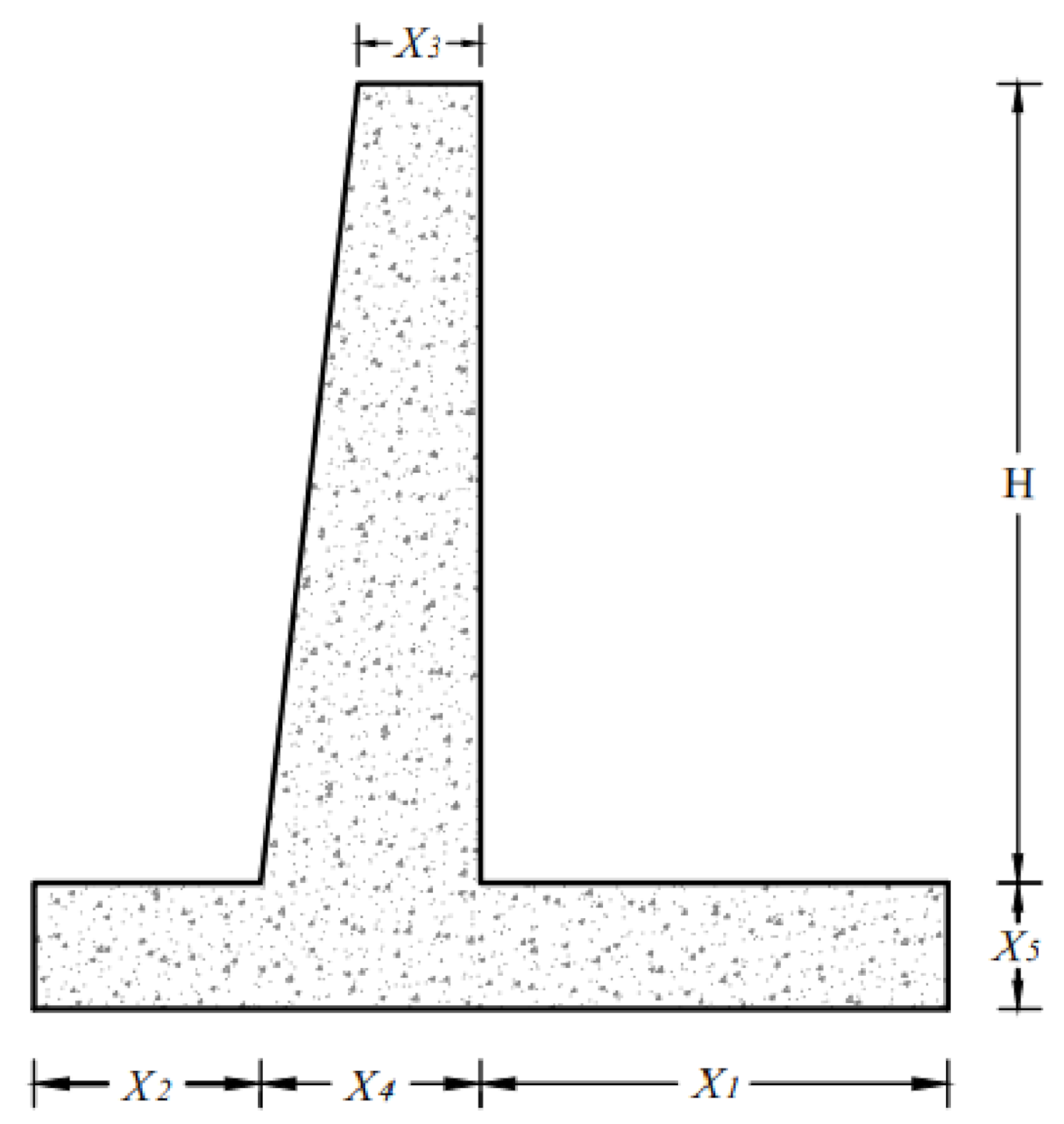
The cross-section of a T-shaped retaining wall is shown in Figure 1 including the design variables and design constants. The definitions of the symbols are listed in

Table 1. Optimization data for T-shaped walls concerning a specific design.

	Definition	Symbol	Limit/Value	Unit
Design Variables	Heel slab/back encasement width of retaining wall	X1	0–10	M
	Toe slab/front encasement width of retaining wall	X2	0–3	M
	Upper part width of cantilever/stem of wall	X3	0.2–3	M
	Bottom part width of cantilever/stem of wall	X4	0.3–3	M
	The thickness of the bottom slab of the retaining wall	X5	0.3–3	M
Design Constants	Difference between the top elevation of bottom-slab with soil in behind of wall (active zone)/stem height	H	6	M
	Weight per unit of volume of back soil of wall (active zone)	γz	18	kN/m3
	Surcharge load in the active zone (on the top elevation of soil)	qa	10	kN/m2
	The angle of internal friction of back soil of wall	Φ	30°
	Allowable bearing value of soil	qsafety	300	kN/m2
	The thickness of granular backfill	tb	0.5	M
	Coefficient of soil reaction	Ksoil	200	MN
	Compressive strength of concrete at 28 days	fc’	25	MPa
	Tensile strength of steel reinforcement	fy	420	MPa
	The elasticity modulus of concrete	Ec	31,000	MPa
	The elasticity modulus of steel	Es	200,000	MPa
	Weight per unit of volume for concrete	γc	25	kN/m3
	Weight per unit of volume for steel	γs	7.85	t/m3
	Width of wall bottom slab	b	1000	Mm
	Concrete unit cost	Cc	50	$/m3
	Steel unit cost	Cs	700	$/ton

. Active and passive stresses occurred according to earth pressures of soil, and external loads are calculated using Rankine earth pressure theory [54]. The objective function is the total material cost of the RC retaining wall, and the aim is to minimize it concerning the design constraints listed in

Table 2. The design constraints

Description	Constraints
Safety for overturning stability	g1(X): FoSot,design ≥ FoSot
Safety for sliding	g2(X): FoSs,design ≥ FoSs
Safety for bearing capacity	g3(X): FoSbc,design ≥ FoSbc
Minimum bearing stress (qmin)	g4(X): qmin ≥ 0
Flexural strength capacities of critical sections (Md)	g5–7(X): Md ≥ Mu
Shear strength capacities of critical sections (Vd)	g8–10(X): Vd ≥ Vu
Minimum reinforcement areas of critical sections (Asmin)	g11–13(X): As ≥ Asmin
Maximum reinforcement areas of critical sections (Asmax)	g14–16(X): As ≤ Asmax

. Also, some coefficients, which are handled to provide the safety of retaining wall, can be seen in

Table 3. ACI 318–14 regulation values utilized in the optimization process.

Load Coefficients in ACI Regulation	Symbol	Value
The coefficient for load increment	Cl	1.7
Reduction coefficient for section bending moment capacity for tension-controlled design	FiM	0.9
Reduction coefficient for section shear load capacity	FiV	0.75
Constant load coefficient	GK	0.9
Live load coefficient	QK	1.6
Horizontal load coefficient	HK	1.6
Safety coefficient for overturning	Osafety	1.5
Safety coefficient for slipping	Ssafety	1.5

. These coefficients and constraints are calculated according to ACI 318: Building Code Requirements for Structural Concrete [55]. If one of the design constraints is violated, the objective function is penalized with a big value. In the design of the RC retaining wall, a tension-controlled design is performed. For that reason, all sections must be designed for the situation that requires a minimum value of 0.005 net tensile strain in the extreme tension steel at nominal strength.

In this section, three different optimization applications are explained: GA, DE, PSO, HS (classic (HS), adaptive (AHS), and adaptive-hybridized (AHHS) versions), FA, ABC, TLBO, FPA, GWO, and JA for minimization of total material cost (concrete and steel reinforcement) for cantilever retaining wall designs. These have consisted of four different cases for wall models individually:

Case 1: Thirty multiple cycles of optimization of design data within Table 1.

Case 2: Thirty multiple cycles of optimization of design data of Case 1, but for different H of the wall.

Case 3: Determination of the best iteration number and population number combination by using different values concerning data in Table 1.

Case 4: Optimization with 20 multiple cycles for different wall parameter combinations given in Table 2.

3.1. Optimization for T-Shaped Wall Designs via Multiple Cycles (Case 1)

In Case 1, optimization processes were carried out for 30 cycles with 20 populations and 5000 iteration numbers to generate optimum wall designs by considering of design values stated in Table 1. The termination criterion is to reach the value of the defined iteration number. Via that criterion, it is also possible to check the number of iterations needed to reach the optimum result. Optimum values of design parameters and objective function with statistical measurements attained in the result of 30 cycles with the usage of 10 metaheuristic algorithms are shown in

Table 4. Optimum design results for Case 1.

Algorithm	X1	X2	X3	X4	X5	Min. Cost	Ave. Cost	Standard Dev.
GA	4.1257	0.0003	0.2003	0.6212	0.4274	428.2421	449.3181	36.9566
DE	4.1323	0.0000	0.2000	0.6098	0.4267	428.1139	433.3653	11.4300
PSO	4.1322	0.0000	0.2000	0.6099	0.4267	428.1139	449.2315	40.6569
HS	4.1197	0.0000	0.2000	0.6222	0.4160	428.2851	429.2780	0.6148
FA	4.1292	0.0000	0.2000	0.6145	0.4266	428.1238	428.1696	0.0294
ABC	4.1315	0.0000	0.2000	0.6135	0.4299	428.1452	431.0378	3.5220
TLBO	4.1323	0.0000	0.2000	0.6099	0.4267	428.1139	428.1139	5.0000 × 10−7
FPA	4.1323	0.0000	0.2000	0.6099	0.4267	428.1139	429.2931	2.1345
GWO	4.0584	0.9320	0.2000	0.6012	0.3800	435.1009	448.5719	9.1413
JA	4.1323	0.0000	0.2000	0.6099	0.4267	428.1139	428.1139	1.2000 × 10−7

. Also, optimization results of HS, AHS, and AHHS where HMCR and FW values are handled as 0.5–0.1, 0.1–0.1 together with random-determined (rand( )), can be seen in

Table 5. Optimum design results provided via HS, AHS, and AHHS for Case 1.

Algorithm	X1	X2	X3	X4	X5	Min. Cost	Ave. Cost	Standard Dev.	HMCR	PAR
HS	4.1308	0.0000	0.2000	0.6078	0.4192	428.2027	429.8543	2.0568	0.5	0.1
	4.1309	0.0000	0.2000	0.6134	0.4245	428.2236	428.7516	1.1862	0.1	0.1
	4.1381	0.0002	0.2000	0.6037	0.4292	428.1761	430.0087	2.2499	rand( )	rand( )
AHS	4.1308	0.0000	0.2000	0.6118	0.4264	428.1151	428.2852	0.9061	0.5	0.1
	4.1354	0.0001	0.2000	0.6053	0.4270	428.1151	428.2852	0.9211	0.1	0.1
	4.1321	0.0000	0.2000	0.6100	0.4266	428.1139	429.4559	2.2556	rand( )	rand( )
AHHS	4.1322	0.0000	0.2000	0.6098	0.4266	428.1139	428.1139	1.7512 × 10−5	0.5	0.1
	4.1323	0.0000	0.2000	0.6098	0.4267	428.1139	428.1143	2.5401 × 10−4	0.1	0.1
	4.1323	0.0000	0.2000	0.6098	0.4267	428.1139	428.1139	2.1047 × 10−5	rand( )	rand( )

. From the results, the optimum design has zero X₂ variables. The front encasement is not required in the optimum design by using the design constants given in Table 1. Only, GA and GWO results have a small non-zero value for X₂, but these algorithms are not effective to find the best optimum result.

On the other hand, according to Table 5, from all of the HMCR–FW combinations, the best results were provided through the usage of random-valued arrangements for each modification of HS. Therefore, for the other following cases, only random-valued arrangements will be evaluated. Additionally, the most effective modification is observed as the random-valued combination of AHHS, so it can reach the minimum cost as an objective function with extremely small deviation compared with all the HS and AHS arrangements.

3.2. Optimization for Wall Designs via Multiple Cycles for H = 10 m (Case 2)

The optimum design of the RC retaining wall is conducted for Case 2 to find an optimum design with front encasement. H value of the wall is taken as 10 m, while all other design properties of the wall and parameters of the optimization process are the same as Case 1, except for iteration number 40,000. The optimum results are given in

Table 6. Optimum design results for Case 2.

Algorithm	X1	X2	X3	X4	X5	Min. Cost	Ave. Cost	Standard Dev.
GA	6.3330	1.4884	0.2000	1.3872	0.7068	1365.3200	1376.4551	32.4525
DE	6.3479	1.4916	0.2000	1.3657	0.7086	1365.2365	1419.9082	1.0055 × 102
PSO	6.3484	1.4914	0.2000	1.3656	0.7086	1365.2388	1458.7287	1.4244 × 104
HS	6.3210	1.4771	0.2000	1.4072	0.7038	1365.7077	1366.2693	0.4286
FA	6.3471	1.4737	0.2000	1.3672	0.7029	1365.3144	1365.3999	0.0561
ABC	6.3534	1.4937	0.2000	1.3584	0.7100	1365.2989	1366.2121	1.6558
TLBO	6.3481	1.4916	0.2000	1.3655	0.7086	1365.2365	1365.2365	2.4953 × 10−5
FPA	6.3483	1.4919	0.2000	1.3651	0.7087	1365.2365	1366.4543	3.8868
GWO	6.3525	1.4440	0.2000	1.3619	0.6999	1365.7193	1376.5011	6.6415
JA	6.3479	1.4916	0.2000	1.3657	0.7086	1365.2365	1365.2366	6.7456 × 10−5

and

Table 7. Optimum design results provided via harmony search (HS), adaptive HS (AHS), and adaptive-hybridized HS (AHHS) for Case 2.

Algorithm	X1	X2	X3	X4	X5	Min. Cost	Ave. Cost	Standard Dev.	HMCR	FW
HS	6.3480	1.4918	0.2000	1.3657	0.7086	1365.2417	1365.3211	0.0509	rand( )
AHS	6.3479	1.4908	0.2000	1.3657	0.7083	1365.2371	1365.2478	0.0081
AHHS	6.3481	1.4914	0.2000	1.3654	0.7085	1365.2365	1365.2369	2.3466 × 10−4

. It can be understood from Table 6 that DE, TLBO, FPA, and JA could reach the minimum cost, but DE deviated from this value with a very high rate along with the cycles. Also, TLBO and especially JA can converge to this value with an extremely minor standard deviation. Both algorithms can be considered as the best options intended for determining optimum design.

On the other hand, HS and AHS are not so effective in terms of reaching the minimum cost. However, AHHS can converge to the minimum cost with a small deviation almost similar to the best algorithms (TLBO and JA).

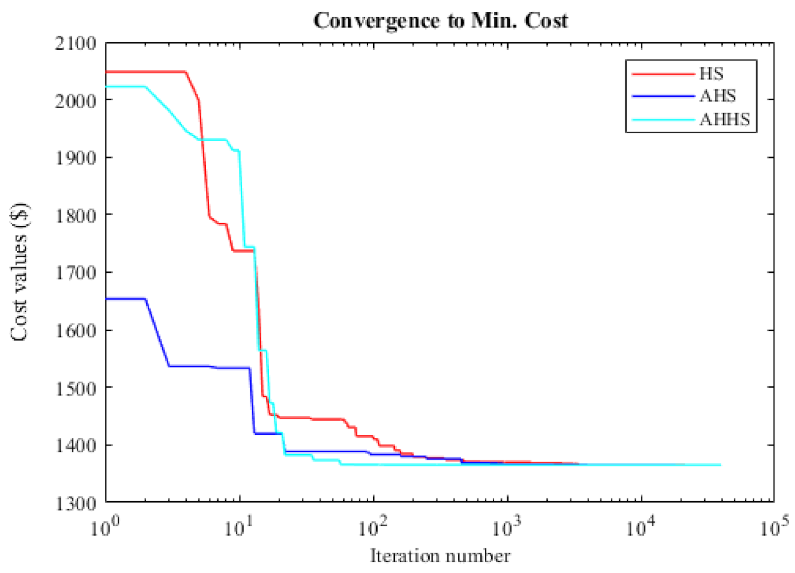
Also, Figure 2 shows convergence behaviors concerning minimum total cost provided in a cycle where the best results are obtained with HS and both modified versions of HS. As can be seen from this figure, reaching the minimum cost level via AHHS, which can find the optimum results and best cost, is realized earlier than the other two methods.

3.3. Best Population and Iteration Numbers for Optimization Processes (Case 3)

In Case 3, the best iteration and population numbers found for determining the optimum design parameters and minimum cost values of retaining wall structures. Accordingly, in all mentioned metaheuristics, the population number is operated as 3, 5, 10, 15, 20, 25, 30, and iteration number is handled from 1 to 5000 increasingly 499, for a specific design comprising from values expressed in Table 1. In this connection, optimum design parameters providing the minimum material cost are found out owing to the determination of the most convenient population together with iteration numbers for each algorithm. These results can be seen in

Table 8. Optimum design values of the wall with the best population-iteration combinations

Algorithm	X1	X2	X3	X4	X5	Min. Cost	Ave. Cost	Standard Dev.	Iter. Num.	Pop. Num.
GA	4.1304	0.0046	0.2001	0.6106	0.4240	428.2186	428.6384	0.3440	2995	15
DE	4.1323	0.0000	0.2000	0.6098	0.4267	428.1139	428.1139	0.0000	1997	30
PSO	4.1324	0.0000	0.2000	0.6096	0.4267	428.1140	699.2741	732.5740	3993	30
HS	4.1356	0.0000	0.2000	0.6110	0.4271	428.3122	432.0160	1.8713	4991	25
FA	4.1331	0.0000	0.2000	0.6078	0.4254	428.1195	428.4955	0.1738	1498	30
ABC	4.1393	0.0000	0.2000	0.5998	0.4269	428.1525	428.7319	0.6954	3494	30
TLBO	4.1323	0.0000	0.2000	0.6098	0.4267	428.1139	428.1139	1.200 × 10−5	4991	25
FPA	4.1323	0.0000	0.2000	0.6099	0.4267	428.1139	428.1139	0.0000	3993	30
GWO	4.0961	0.3437	0.2000	0.6020	0.3762	434.2075	457.4451	9.1502	2496	30
JA	4.1323	0.0000	0.2000	0.6099	0.4267	428.1139	428.1139	5.000 × 10−6	4492	25

and

Table 9. Optimum design values of the wall provided via HS, AHS, and AHHS with the best population-iteration combinations.

Algorithm	X1	X2	X3	X4	X5	Min. Cost	Ave. Cost	Standard Dev.	Iter. Num.	Pop. Num.	HMCR	PAR
HS	4.1281	0.0000	0.2000	0.6164	0.4265	428.1428	428.4236	0.1856	2995	25	rand( )
AHS	4.1326	0.0000	0.2000	0.6094	0.4267	428.1143	428.1207	0.0055	4492	25
AHHS	4.1323	0.0000	0.2000	0.6097	0.4267	428.1139	428.1139	7.600 × 10−6	4492	10

.

As is shown in the tables above, the minimum cost can be obtained via DE, TLBO, FPA, JA, and AHHS. However, it is so clear that the standard deviation of the AHHS result has an extremely low rate when this cost value is determined, besides the population number is smaller than the other most effective algorithm, JA. AHHS can reach the optimum result with a smaller number of the analysis that is calculated by multiplying the population number with the iteration number for all algorithms other than TLBO since it is double this value for TLBO that employs two phases in an iteration.

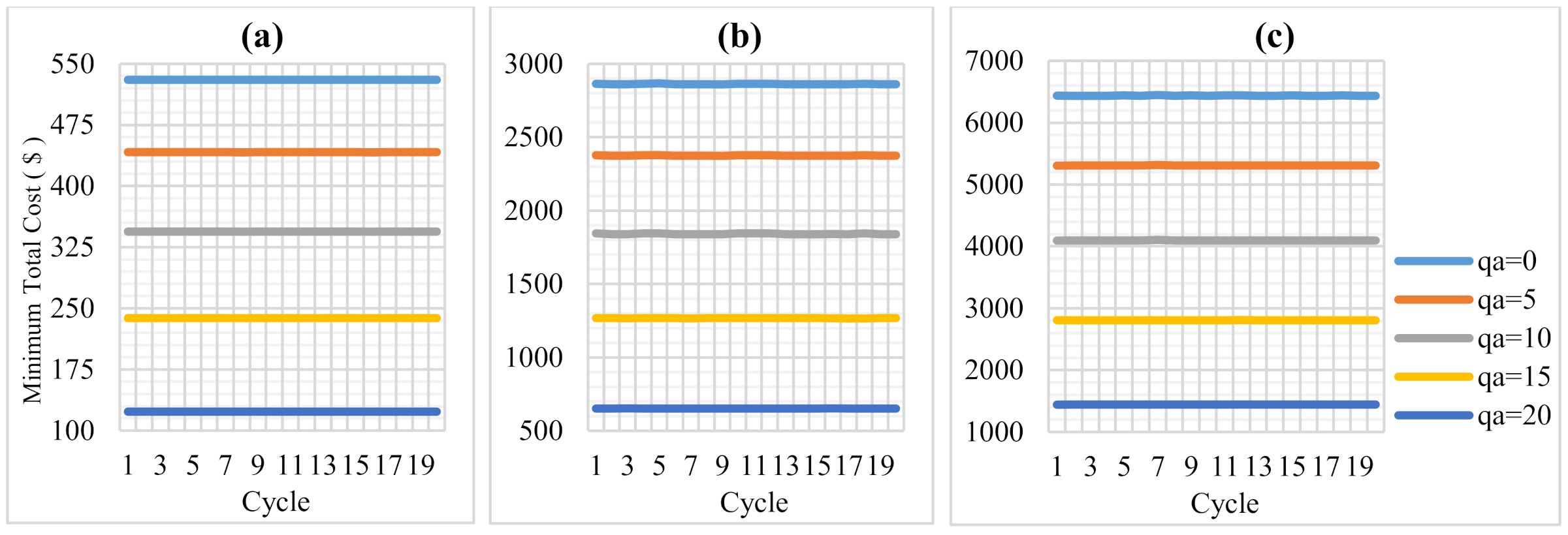
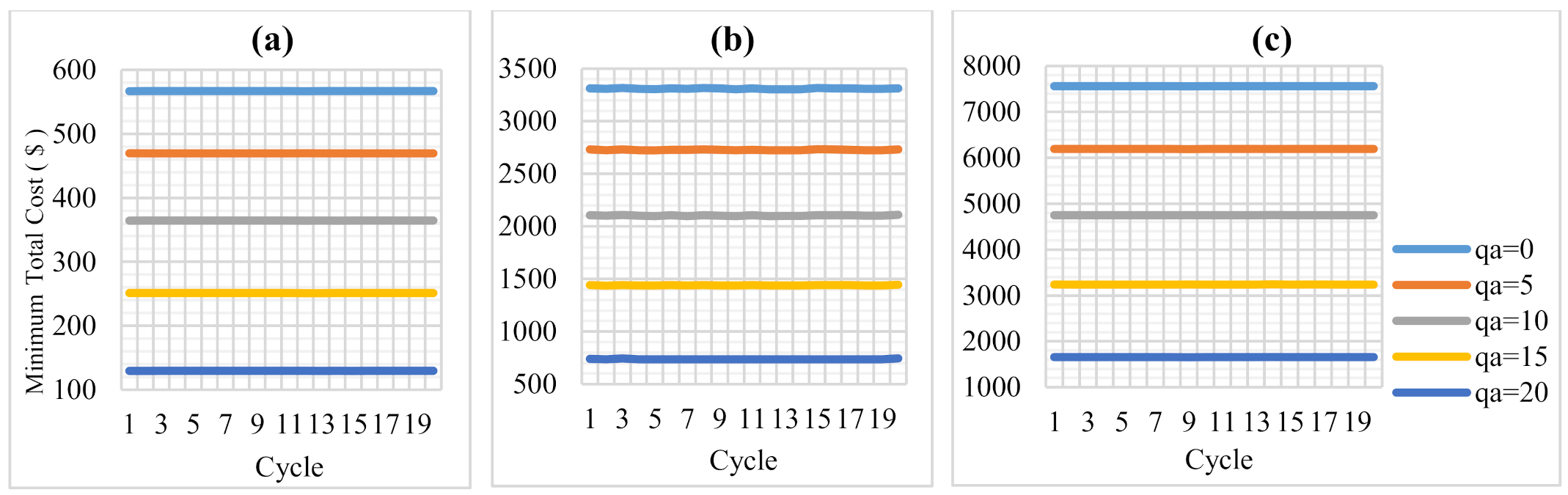
3.4. Optimum Analysis for Different Wall Structure Variations with Multiple Cycles (Case 4)

Finally, numerous retaining wall models are generated employing different ranges for three design constants including stem height (H), soil weight per unit weight of volume for wall back soil (γ_z), and surcharge load on the top elevation of soil (q_a). These constants and their properties are summarized in

Table 10. Range values of design constants used in the optimization process.

Symbol	Ranges	Increment	Unit
H	3–10	1	M
γz	16–22	1	kN/m3
qa	0–20	5	kN/m2

.

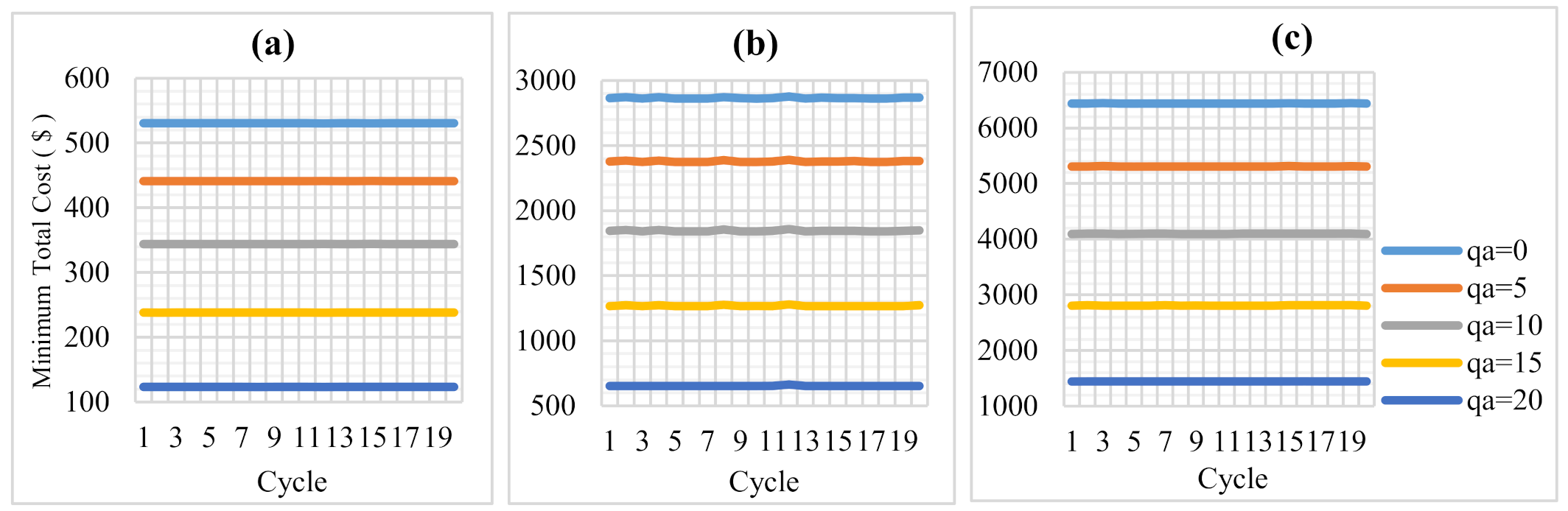
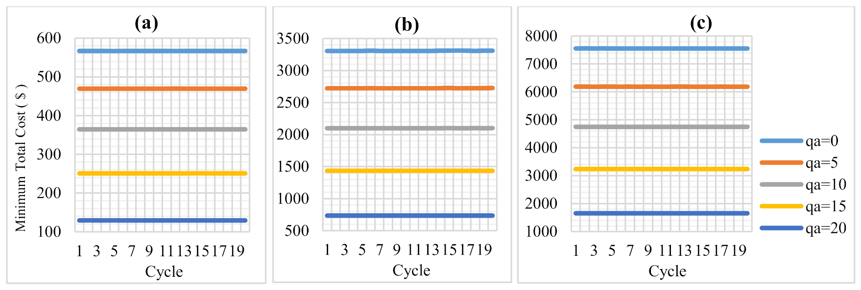
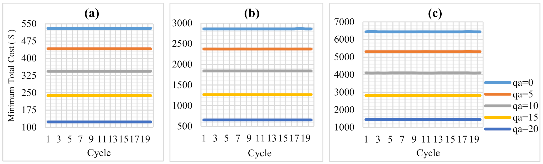
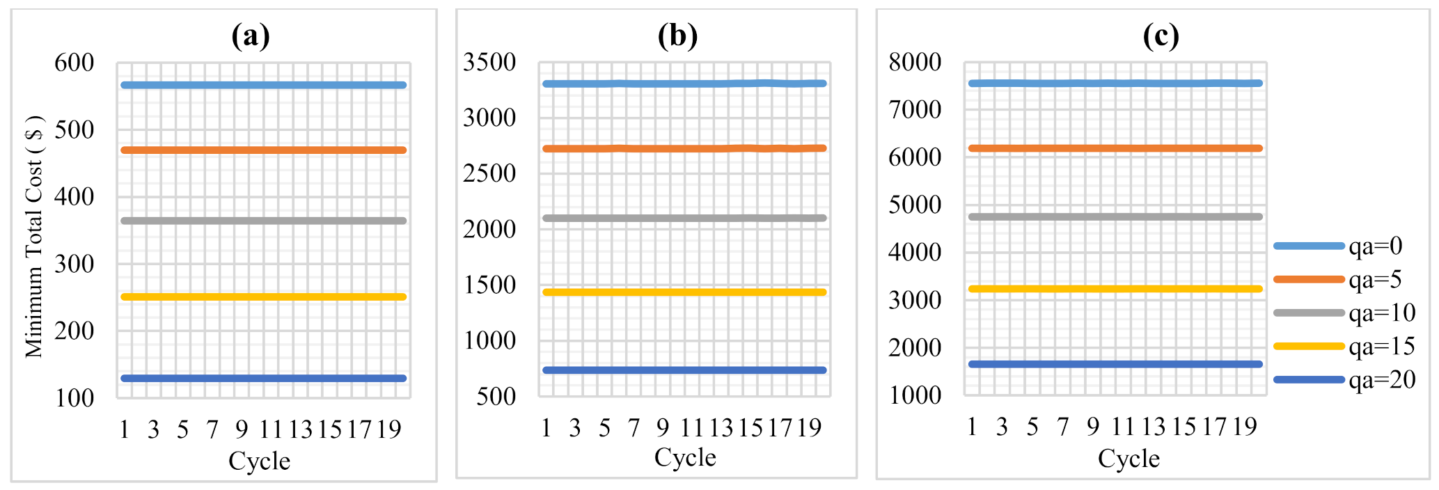
Also, for both modifications of HS together with the classical version of itself, 20 cycles are performed with values of Case 1 as the same population and iteration numbers during optimization application. In Figure 3, Figure 4, Figure 5, Figure 6, Figure 7 and Figure 8, analysis results are presented for HS, AHS, and AHHS, respectively. These are generated according to the minimum and maximum value of γ_z as 16 and 22 kN/m³ and three different H including 3, 7, and 10 m for each q_a to understand the deviation of cost values in each cycle.

According to the results of HS, it can be recognized that the obvious fluctuations for minimum cost results occur in γ_z = 16 kN/m³ and 5 and 10 kN/m² q_a values for 7 m wall height. There are no great changes in costs for other wall heights and q_a values according to the increasing of cycles.

On the other hand, for AHS, minimum costs provided in sequent cycles for γ_z = 16 kN/m³ with 7 m wall height in 0 and 10 kN/m² (q_a), occur as unstable/wavy. Also, in AHHS analysis results, it can be said that there is so small change for minimum cost intended for only one design parameter combination as γ_z = 16 kN/m³, H = 10 m with q_a = 0 kN/m². In general, classical HS and modified versions are effective in this evaluation.

4. Conclusions

4.1. Case 1

In Case 1, optimum design variables and minimum cost were obtained for a specific design through performing 30 cycles. The best result as minimum cost value can be provided via DE, PSO, FPA, TLBO, and JA. However, the most effective ones are JA (first) and TLBO (second) because the standard deviation of both best results provided via themselves are the smallest ones, respectively. These two methods can be the most effective and useful ones for the stability of optimization results. Standard deviation values belonging to DE and PSO especially were quite large, and could cause change of optimum values in every analysis. Thus, DE and PSO are not consistent and the mentioned two new generation algorithms can be accepted as effective and stable for this structure model. The optimum design has zero toe slab/front encasement width of retaining wall, and all algorithms other than GA and GWO are effective to find this solution. Additionally, AHS and AHHS are successful to reach the minimum cost through the usage of random-determined parameters and all of the parameter combinations, respectively. In particular, AHHS possesses a considerable performance in performing this due to showing relatively small deviations.

4.2. Case 2

Case 2 was carried out like Case 1 by considering the wall height (H) as 10 m. Optimization results were ensured with the usage of the same parameters (except for iteration numbers such as 40,000) expressed in Table 1. Different from Case 1, the optimum result of the front encasement (X₂) is not zero. As seen in Table 6, although DE, TLBO, FPA, and JA are effective to find the best objective function as minimum total cost, DE has a big error/deviation rate. This may cause to occur optimum costs at varying values. The most effective methods are TLBO and JA in terms of the finding of the best cost with a very small deviation. Moreover, FPA is also successful at this issue but can approach the minimum cost result with a slightly high deviation. As to HS modifications, the best result as $1365.2365 can be observed in operation performed via only AHHS, which consists of HS and JA. A similar result can be found in the performance with TLBO and JA in terms of smallness of standard deviation. Also, the proposed hybrid algorithm has a better convergence ability than HS and AHS. For the difference between the best and average results, the hybrid method has a very small difference compared to the others.

4.3. Case 3

In Case 3, the optimization process was performed by using different iteration and population numbers to find the best parameter combinations. According to the obtained results (Table 8), DE and FPA have equal performance in terms of minimizing the cost, and JA and TLBO are the best algorithms towards the aim of this process. However, there is a significant point for the best iteration number that DE is better than FPA as 1997 iterations. Both required iterations and population numbers are almost the same for TLBO and JA. When they are compared, JA’s deviation is smaller than TLBO’s one. In a summary, DE is very effective for providing optimum values and prohibits loss of time. As the second alternative method, FPA can be preferred due to the equivalent small deviation and less iteration number. It proves that the best pick of the population and iteration number plays an important role in the performance increase by DE and FPA. According to the results of HS and its modifications, only AHHS can be successful for detection of the minimum cost as $428.1139 with a very small standard deviation. From the results, AHHS is the best among all of the metaheuristics for this case because of the extremely low population number of 10, compared with the other values such as 25 and 30. That is why AHHS provides a speed increase in reaching the optimum values comparing to other ones, while the other advantages are slightly equal with the best ones.

4.4. Case 4

In Case 4, minimum costs and optimum design variables were determined for retaining wall designs modeled by using different value ranges for the design constants. The results were evaluated concerning two different values of γ_z (minimum 16 kN/m³, maximum 22 kN/m³) and minimum, average, and maximum values of H. Only HS and its modified versions, which are developed in the current study, were evaluated, and Figure 3, Figure 4, Figure 5, Figure 6, Figure 7 and Figure 8 were presented to show the fluctuation of minimum costs for specific designs by the usage of some values of q_a, by regarding HS, AHS, and AHHS, respectively. It can be seen that in analysis results made for the modified versions the deviations occur in only 16 kN/m³ value of γ_z for all wall height combinations. It means that since γ_z increases, minimum cost deviations for different designs generated with various wall heights do not appear for any q_a. Also, according to the results of HS, AHS, and AHHS for 16 kN/m³, it can be seen that the deviations for costs along 20 cycles are the most apparent in classical HS and AHS with 0 and 10 for q_a and 7 m wall height (H), respectively. Consequently, in Case 4, the most effective and usable algorithm is AHHS for the wall designs in terms of both stability of objective function values and the true value of minimum costs without almost fluctuation for costs.

4.5. General Advantages of AHHS

It is noticed that AHHS is also quite effective and can provide optimum design variables with the minimization of total cost in all Cases 1, 2, and 3. According to this performance, it is possible to say that AHHS is a competitive method. The robustness of the algorithm and success for the local optima problem was provided via obtaining very small standard deviation results for multiple runs, while most of the classical methods have big values for standard deviation. The essential performance of the algorithm is realized for the computational effort value due to having a smaller number of iterations than the others for reaching the final optimum results. Furthermore, AHHS can be used as a user-defined parameter-free algorithm by assigning the parameter with a random number. The analysis results done with randomly assign initial parameters of HMCR and FW provided that AHHS was not affected by the choice of the parameter. Also, the best performance is obtained via using random parameters. In that case, being an adaptive algorithm plays an important role in this performance.