Study on the Spatial Association and Influencing Factors of Carbon Emissions from the Chinese Construction Industry

Abstract

As the world’s largest carbon emitter, China is under enormous pressure to decrease carbon emissions. With the economic development in recent years, China has increased its investment in infrastructure, and the construction industry has become an essential source of carbon emissions. Using the social network analysis (SNA) methodology, this article analyzes the evolutionary characteristics of the spatial correlation network for carbon emissions in the construction industry from 2003–2017 and its affecting factors. The results of the empirical analysis in this paper are: (1) the spatial association of carbon emissions in Chinese inter-provincial construction industry shows an intuitive network layout and the spatial network has gradually stabilized since 2014; (2) according to the results of degree centrality, betweenness centrality and closeness centrality, it can be concluded that the regions with higher level of association with other provinces are the central and the eastern regions (Henan, Hubei, Hunan, Guangdong, Jiangsu, etc.) and Xinjiang; the linkage of construction-related carbon emissions was mainly achieved through the regions of Henan, Anhui, Shanxi, Hebei, Guangdong, and Inner Mongolia; the regions with higher level of construction industry development (Jiangsu, Henan, Hunan, Guangdong, etc.) are more closely associated with other provinces; (3) geographical proximity and reduction of difference in energy intensity and in industrial structure have substantial positive effects on the carbon emission association of the construction industry. Finally, based on the research results, this article proposes corresponding policy recommendations.

1. Introduction

Global climate governance is of particular relevance as the adverse impact of greenhouse gas (GHG) emissions on the ecological environment and the health of residents [1,2,3,4]. With rapid economic growth since the 21st century, a considerable number of resources and energy have been consumed, making China the world’s largest energy consumer and GHG emitter [5]. Carbon dioxide (CO₂) is the most significant anthropogenic greenhouse gas in the environment [6]. These serious climatic problems and environmental issues triggered by GHG have aroused the attention of the Chinese government to introduce a series of carbon emission reduction policies [7]. With the increased investment in infrastructure, the construction industry has become a significant source of carbon emissions in China and needs further attention in the development of a low-carbon economy [8,9,10]. Previous studies have shown here that the construction sector accounts for much more than 40% to world energy consumption as well as 36% of global carbon emissions [11]. China’s construction sector occupies a crucial position in the national economies, consuming 10.5–11.3 billion tons of coal equivalent, contributing as much as 28–30% of the country’s total carbon emissions [12]. Moreover, due to rapid urbanization and industrialization, plus economic development, China’s construction industry is facing tremendous carbon emission reduction stresses. Simultaneously, there is still excellent abatement potential for this industry [13,14,15,16]. Therefore, for both China and the world, the carbon emissions mitigation in the Chinese construction industry is of substantial implications.

Regional economic imbalance, low carbon technology level, and other factors lead to the spatial heterogeneity for carbon emissions and the complexity of spatial associations in the construction industry, which pose a challenge to regionally coordinated carbon emission reduction [17]. Furthermore, carbon emissions have spillover effects, which are not just an ambient issue for a particular district but may also be transported to several other districts via climate ingredients and economic behavior, including atmospheric flows and industrial transfer [18,19]. Therefore, a complete understanding of the space network structure of carbon emissions from the construction industry among Chinese provinces, determining the roles of different regions in the spatial correlation network and analyzing the driving factors of CO₂ emissions spatial correlation, is necessary. Most of China’s local policies and allocation targets for carbon emissions are based on each province’s direct emissions, and the links between regions were seldom considered [20]. The study of spatial association features and evolution rules of the regional construction industry can help the devising of regional low-carbon development policies.

The study of the regional system has developed in recent years from regional attribute analysis to regional network research, with an emphasis on space network correlation behavior [21,22]. The most used method applied in this analytical framework is social network analysis (SNA). When representing complex associations in SNA, researchers usually use an association matrix, which not only exposes the characteristics of the association network from an attribute data point of view but also identifies the relationships that exist between nodes in the network from a relational data point of view [23]. Most of the traditional spatial measurement methods use attribute data, which are hard to classify in relation to the entire network structure of a spatial association of carbon emissions, and its impact can only be studied by “quantity” rather than “relationship” [24]. Due to network data frequently encountering problems as with multicollinearity and autocorrelation, the quadratic assignment protocol (QAP) is considered more amenable than other approaches for the regression analysis of impact variables [25].

This research complements previous studies of the construction industry’s carbon emissions since we first included SNA into a spatial correlation study among this framework. This method outperforms existing methods in terms of analyzing the correlated evolution of the spatial associations among emission networks in China’s interprovincial construction sector and reveals ways of effect by different provinces. The results presented in this paper are intended to provide a foundation for the regional collaborative reduction strategies for the construction industry. In this article, we use applicable data from 2003 to 2017 in the different provinces of China and build a modified gravity model to study the spatial correlation of construction CO₂ emissions within China from the perspective of the social network. Based on the modified gravity matrix, we researched the features of the spatial correlation network and its driving ingredients. Finally, we make policy recommendations for the collaborative governance of carbon emissions from the construction industry of each province based on our analysis results.

The article is organized into six sections. The related literature is discussed in Section 2. The methods used to analyze the carbon emissions spatial association of Chinese construction are defined in Section 3. The results are summarized in Section 4. We discuss the research results in Section 5. The research conclusions and the policy recommendations are presented in Section 6.

2. Literature Review

Spatial analysis is becoming the mainstream method used to provide a scientific basis for regional low-carbon policies. Through the growth of spatial econometric research and SNA, more and more academics are paying attention to the spatial correlation characteristics of connected networks from these two perspectives.

First, some studies used spatial correlation to assess the spatial econometric effects of pollutants. Although spatial weight matrix was incorporated in these studies, the other underlying data were attributed data. Except for the spatial weight matrix which represents the geographical relationship among provinces, other variable data cannot describe the inter-provincial correlation effect properly [26]. For instance, by introducing the global and the local Moran I exponents, researchers notice the evident positive spatial association between Chinese regional CO₂ emissions, and spatial agglomeration features exist [27,28,29,30,31,32,33]. However, Han et al. (2018) concluded that a gravity model combining geographic and economic distances presented significantly higher spatial correlations of carbon emissions than a simple matrix of geographic and economic distances [18]. Therefore, for carbon emission, we are more likely to see a significant correlation in areas that are geographically close and economically interconnected.

Second, the other category of studies employs the SNA approach to analyze the carbon emissions spatial correlation properties [34,35,36,37,38]. These studies define the spatial association between sample regions by the vector autoregression (VAR) approach or the gravity model, then create a network of spatial associations across all regions and investigate the features of CO₂ emissions spatial associations. Relational data are utilized in this method to study the interrelationships that exist between provinces and the spatial correlation from the perspective of the system’s structure rather than a single region. This approach takes into consideration both holism and individualism, of which the whole configuration of the network and the unique features of the regions may be investigated. For instance, Wang et al. (2018) used this approach to research particularly the structure of the CO₂ network in Chinese regions and the ingredients affecting the CO₂ emissions spatial correlation; findings show that regional emissions of carbon are an intuitive network of spatial connections [39]. He et al. (2020) conducted SNA to research the spatial network structure and the spatial correlation effects of carbon emissions from the electricity sector in China from 2005 to 2016; the results indicate that the space network structure of CO₂ emissions from the electricity sector presents an apparent network structure and the spatial correlation of carbon emissions is relatively stable, and regions are closely connected [24].

The two kinds of research mentioned above are essential to the comprehension of the spatial correlation properties for carbon emissions. While both approaches could be applied to spatial interaction research, SNA occupies distinct advantages. First, the SNA approach is mainly based on relational data instead of attribute data to describe the relationships in space, and it studies the relationships between objects in the network rather than individual characteristics. Relational data have the advantage of directly reflecting association features, which is beneficial to the construction of spatial correlation networks and can give concise and intuitive visual analysis. Second, the QAP analysis method in SNA allows correlation analysis among the spatial association matrix and possible driven ingredients, which facilitates the identification of influence factors that significantly affect spatial associations [36]. It is worth mentioning that QAP obtains the estimation results by multiple permutations of the random permutation matrix, thus avoiding the multicollinearity problem that often occurs when using the traditional ordinary least squares (OLS) method [40]. Additionally, methods for spatial econometric analyses are highly spatial weight matrix-based, but different matrices of spatial weight can result in different results. Similarly, SNA does not necessarily involve using a specific method for constructing a spatial association matrix. Errors also occur when building correlations based on gravity models. However, the procedure for modification of the model using the geometric average value could significantly minimize the influence of an individual index on the entire results and can be used to obtain the network structure’s evolution trend.

Based on previous studies, the main contributions of this paper are as follows. By introducing the SNA method, we analyzed the evolution of the spatial association of inter-provincial construction industry emissions in China and revealed the influence pathways of the inter-provincial emission association network, thus providing a scientific basis for the formulation of regional collaborative emission reduction policies for the construction industry in China. Specifically, this paper first obtains the carbon emission spatial correlation matrix by constructing a modified gravity model. Second, the SNA method is introduced into the analysis of the spatial association of CO₂ emissions from the construction sector, and the structure of the CO₂ emission association network can be presented more intuitively through social networks. In addition, we applied the QAP regression analysis approach to research the driving ingredients for the carbon emission spatial network, essentially avoiding the problem of multicollinearity caused by multiple independent variables, providing a more scientific and reasonable analysis.

3. Methodology and Data

China’s inter-provincial construction CO₂ emission spatial association network gathers all inter-regional CO₂ emission spatial connections [41]. In the network, each node refers to a different province, and the connections between nodes represent the spatial correlation of inter-provincial construction industry carbon emissions. The research steps of this article are as follows: first, by constructing a corrected gravitational model, we obtained the spatial correlation network matrix and used UCINET software to research the features of the network as a whole and individual provinces; second, based on the constructed spatial association network matrix and the graph theory, we calculated degree, betweenness, and closeness centrality of each node. Then, QAP correlation and regression analyses were used to determine the significant affecting factors of the spatial correlation network.

The SNA method enables the analysis of a region as a whole by establishing an association network between actors and also by conducting a comparative study of the individuals in the network from a partial perspective [42]. The spatial correlation analysis can help identify which factors better explain the complexity of carbon emission correlation networks. Therefore, the SNA method was used in this study because of its advantages over traditional measures in analyzing interprovincial differences.

3.1. The Modified Gravity Model

The study of the SNA is based on the matrix of correlation between the nodes that are often calculated via the causality test of Granger on the basis of the VAR approach or by the gravity model. VAR’s susceptibility to time lag makes it only suitable for data spanning a long time, thus VAR should not be applied to cross-sectional data or to expose different evolution characteristics of the network architecture [40]. The gravity model overcomes this shortcoming and is more conducive to portraying the evolution pattern of the spatial association network of CO₂ emissions in the construction industry. This study incorporates the gravity model in the area of CO₂ emissions for the construction sector based on the abovementioned considerations:

$${\mathrm{G}}_{\mathrm{i}\mathrm{j}}=\mathrm{k}\frac{{\mathrm{M}}_{\mathrm{i}}{\mathrm{M}}_{\mathrm{j}}}{{\mathrm{D}}_{\mathrm{i}\mathrm{j}}^{\mathrm{b}}}$$

(1)

where G_ij is the gravitational value between objects i and j, M_i and M_j are their “mass”, D_ij is the specific distance between i and j, b is the distance attenuation coefficient; additionally, k is a constant based on experience.

Geographical proximity and economic importance are critical variables that have an impact on the spatial structure of economic operations, contributing directly to a growth of the demand for energy and producing large emissions of CO₂ [43]. Therefore, geographic proximity and economic proximity should both be considered when establishing the correlation network of CO₂ emissions for the construction sector, and the “mass” of construction CO₂ emissions for the gravity model is modified. We refined the conventional gravitational model on the basis of the associated variables so that it can be applicable to the development of CO₂ emission linkages in the construction industry. As follows, the basic model is:

$${\mathrm{c}}_{\mathrm{i}\mathrm{j}}=\frac{{\mathrm{T}}_{\mathrm{i}}}{\left({\mathrm{T}}_{\mathrm{i}}+{\mathrm{T}}_{\mathrm{j}}\right)}\times \frac{\sqrt[3]{{\mathrm{P}}_{\mathrm{i}}\times {\mathrm{T}}_{\mathrm{i}}\times {\mathrm{E}}_{\mathrm{i}}}\times \sqrt[3]{{\mathrm{P}}_{\mathrm{j}}\times {\mathrm{T}}_{\mathrm{j}}\times {\mathrm{E}}_{\mathrm{j}}}}{{\mathrm{D}}_{\mathrm{i}\mathrm{j}}{}^2}$$

(2)

where c_ij represents the correlation between carbon emissions from construction in province i and province j, T is the total carbon emissions from the construction industry, P is the population size, E is the regional GDP, D_ij is the geographical distance between provincial capital i and j; for the choice of distance centers, in addition to referring to previous studies, we justified the choice by analyzing the carbon emission data of cities in each province (see Appendix A). k = $\frac{{\mathrm{T}}_{\mathrm{i}}}{\left({\mathrm{T}}_{\mathrm{i}}+{\mathrm{T}}_{\mathrm{j}}\right)}$ is the empirical constant, expressed by the proportion of carbon emissions in construction of province i to the sum of construction carbon emissions of provinces i and j, which represents the structural difference in CO₂ emission control between regions [34].

The gravitational matrix between the 30 provinces can be obtained from model (2):

$${\mathrm{G}}_{\mathrm{i}\mathrm{j}}={\mathrm{G}}_{30\times 30}=\left(\begin{array}{cccc}{\mathrm{c}}_{1,1}& {\mathrm{c}}_{1,2}& \dots & {\mathrm{c}}_{1,30}\\ {\mathrm{c}}_{2,1}& {\mathrm{c}}_{2,2}& \dots & {\mathrm{c}}_{2,30}\\ \dots & \dots & \dots & \dots \\ {\mathrm{c}}_{30,1}& {\mathrm{c}}_{30,2}& \dots & {\mathrm{c}}_{30,30}\end{array}\right)$$

(3)

After obtaining the gravity matrix (G = (G_ij)), the average value of each row of the gravity matrix is calculated as the threshold value. If c_ij is smaller than the line average, the CO₂ emissions of provinces i and j are not correlated. On the other hand, if c_ij is greater than the row average, there is a link between the CO₂ emissions of provinces i and j, and the position of the line in the spatial network can be drawn from province i to j. If the value of gravity between the two provinces is greater than this threshold, it means that there is a strong correlation of carbon emissions between the two provinces, and the value is 1; otherwise, the value is 0.

3.2. Network Characterization Index

Identifying the most influential nodes in the network and evaluating the centrality of the network are two main objectives of SNA [33]. In terms of the overall network features, centrality and spatial clustering, the network can be evaluated, and the methods used in this section are based on Scott’s book, “Social Network Analysis: A Handbook” (2007) [40]. Network access represents the network structure’s robustness and weakness. For connectedness, the calculation formula used is:

$$\mathrm{C}=1-\frac{\mathrm{V}}{\mathrm{N}\times \left(\mathrm{N}-1\right)/2}$$

(4)

where C is the connectivity, V is the number of unreachable pairs of points in the network, and N is the number of network nodes.

The network density indicates how tightly connected the spatial network is, and the higher the network density is, the greater the correlation of the network is. The formula here is:

$$\mathrm{D}=\frac{\mathrm{L}}{\mathrm{N}\times \left(\mathrm{N}-1\right)}$$

(5)

where D is the network density, L is the number of network relationships, and N(N-1) is the maximum number of possible network relationships.

Network efficiency reflects the degree of redundancy of inter-provincial network connections—the lower the efficiency of the network is, more frequently do the inter-provincial connections occur and the smaller the room is for CO₂ emissions. The calculation formula is as follows:

$$\mathrm{E}=1-\frac{\mathrm{M}}{\max \left(\mathrm{M}\right)}$$

(6)

where E is the network efficiency, M is the number of redundant lines in the network, and max (M) is the actual number of lines that can be redundant in the network.

The hierarchy of the network represents the supremacy position of the network members in the network. The higher the value is, the more nodes in the edge position are present. The formula here is:

$$\mathrm{H}=1-\frac{\mathrm{K}}{\max \left(\mathrm{K}\right)}$$

(7)

where H is the network hierarchy, K is the number of symmetrically reachable node pairs in the network, and max (K) is the maximum number of symmetrically reachable node pairs in the network.

3.3. Centrality Analysis Index

Centrality is a valid index that measures the position and the function of individuals in a network and is widely used in social network analysis, which can help better understand the importance of the roles played by individual provinces in the associated network and thus help formulate regional policies accordingly. Centrality represents the position and the function of each network node and what kind of central position it occupies, including degree centrality, betweenness centrality, and closeness centrality. In the network centrality analysis, the centrality of each node measures the “power” of an individual in the whole network, and the larger the value is, the more a province is related to other regions in the network, and the greater the network is constructed around this province.

The degree centrality of each node in the network is the number of other points that are directly connected to that point. If a point has a high centrality, it means that a province is directly connected to several provinces in the CO₂ emission correlation network and is closer to the center of the network. It is expressed as follows:

$$\mathrm{D}\mathrm{e}=\frac{\mathrm{n}}{\mathrm{N}-1}$$

(8)

where De is the degree centrality of the province, n is the number of regions directly connected with the target region, and N is the number of entire regions in the network.

Betweenness centrality is defined as the degree to which a node controls the relationships between other nodes. Specifically, if a province is on a geodesic (shortest path) between many other provinces, that point has a high degree of betweenness centrality. The greater its importance is, the greater are the province’s superiority and its power to regulate ties with other provinces. The formula here is:

$${\mathrm{C}}_{\mathrm{A}\mathrm{B}\mathrm{i}}=\frac{2{\displaystyle \sum _{\mathrm{j}=1}^{\mathrm{n}-1}{\displaystyle \sum _{\mathrm{k}=2}^{\mathrm{n}}{\mathrm{b}}_{\mathrm{j}\mathrm{k}}\left(\mathrm{i}\right)}}}{{\mathrm{n}}^2-3\mathrm{n}+2},\mathrm{j}\ne \mathrm{k}\ne \mathrm{i},\mathrm{a}\mathrm{n}\mathrm{d} \mathrm{j}<\mathrm{k}$$

(9)

where C_ABi is the betweenness centrality of province i, b_jk(i) denotes the ability of province i to control the association of two points in province j and province k, and is equal to the probability that province i is on a shortcut between province j and province k, i.e., ${\mathrm{b}}_{\mathrm{j}\mathrm{k}}(\mathrm{i})={\mathrm{p}}_{\mathrm{j}\mathrm{k}}(\mathrm{i})/{\mathrm{p}}_{\mathrm{j}\mathrm{k}}$, where p_jk(i) represents the number of shortcuts that exist between province j and province k through province i.

In addition to degree centrality and betweenness centrality, another indicator that portrays the central position of a point is closeness centrality. The centrality of the closeness measures the sum of the shortcut distances between a node and all other nodes in the network. In our carbon emission correlation network of the construction industry, if the “distance” between a province and all other provinces is very short, it can be considered that the province has a high degree of closeness centrality. The expression is as follows:

$${\mathrm{C}}_{\mathrm{A}\mathrm{P}\mathrm{i}}^{-1}={\displaystyle \sum _{\mathrm{j}=1}^{\mathrm{n}}{\mathrm{d}}_{\mathrm{i}\mathrm{j}}}$$

(10)

where ${\mathrm{C}}_{\mathrm{A}\mathrm{P}\mathrm{i}}^{-1}$ is the closeness centrality of province i in the association network, and d_ij is the shortcut distance between province i and province j (i.e., the number of edges contained in the shortcut).

3.4. QAP Relationship Hypothesis Testing

In order to analyze the affecting factors of the spatial correlation of carbon emissions for the Chinese construction industry, we introduced QAP correlation analysis and regression analysis methods. The specific calculation is divided into two steps. Firstly, the correlation between the dependent variable and the influencing factor is analyzed, and the influencing factors with significant correlation are obtained; secondly, the significant variables obtained by the correlation analysis are brought into the QAP regression analysis model, and each row and column of the dependent variables is stochastically replaced at the same time; finally, the regression result of the related influencing factors of the construction industry carbon emission spatial association matrix is obtained.

The construction sector’s spatial carbon emissions are impacted by several factors, and it is also critical that policymakers recognize influencing factors and implement more focused strategies to minimize provincial pollution. Lu et al. (2020) demonstrated that there is a spatial spillover effect of carbon emissions from the construction industry in China through a spatial econometric regression model and that factors such as economic level, energy intensity, industrial structure, and industrial agglomeration level have observably spatial spillover effects on CO₂ emissions from the construction industry [17]. Yang et al. (2019) analyzed the spatial data to conclude that air pollution in China exhibits significant spatial spillover effects and spatial agglomeration characteristics, and the input of environmental management has a significant inhibitory effect on air pollution [44]. According to the related research and data availability, we set up the model on the basis of the analysis above:

$$\mathrm{T}=\mathrm{f}\left(\mathrm{D},\Delta \mathrm{P}\mathrm{G}\mathrm{D}\mathrm{P},\Delta \mathrm{E}\mathrm{I},\Delta \mathrm{I}\mathrm{S},\Delta \mathrm{I}\mathrm{A},\Delta \mathrm{E}\mathrm{R}\mathrm{I}\right)$$

(11)

where T represents carbon emissions spatial correlation matrix for the construction industry in China, which can be obtained by symmetrizing the spatial gravity matrix; D refers to the geographical adjacency matrix of provinces; $\Delta \mathrm{P}\mathrm{G}\mathrm{D}\mathrm{P}$ is the difference in economic development, which is expressed by the difference in GDP per capita of each province; $\Delta \mathrm{E}\mathrm{I}$ refers to the interprovincial differences in energy intensity of the construction industry; $\Delta \mathrm{I}\mathrm{S}$ is the difference of industrial structure in the construction industry by provinces; $\Delta \mathrm{I}\mathrm{A}$ refers to the interprovincial differences in construction industry agglomeration; rep $\Delta \mathrm{E}\mathrm{R}\mathrm{I}$ resents the difference in environmental regulation intensity in the construction industry by provinces. The detailed definition and calculation method of relevant variables in the model are shown in

Table 1. Variables and data definitions.

Variable	Description	Definition
T	carbon emission spatial correlation	Spatial correlation matrix obtained by the modified gravity model
D	Geographical Adjacency	If there are two neighboring provinces, its value is set to 1; if there are no adjacent provinces, its value is set to 0
ΔPGDP	Difference in Economic Development	PGDP = GDP of each province/total population in each province
ΔEI	Difference in Energy Intensity	EI = energy consumption in each province’s construction sector/total output value in the construction sector of each province
ΔIS	Difference in Industrial structure	IS = construction sector output of each province/total national output value of construction industry
ΔIA	Difference in Industrial agglomeration	IA = (c/q)/(cT/qT), where c represents the construction industry output value of each province, q refers to each province’s total output, cT represents national construction industry total output, qT represents the total national output
ΔERI	Difference in Environmental Regulation Intensity	ERI = R/c, where R represents the total pollution control investment of each province, c refers to construction industry output value in each province

.

3.5. Data Sources

This paper researched the spatial correlation network of CO₂ emissions in the construction industry from 2013–2017 using Chinese provinces as network nodes. Considering the availability of data, the study only included 30 provinces; Tibet, Hong Kong, Macao, and Taiwan were not included. The relevant data needed for this analysis were mainly the CO₂ emissions from the construction sector in each province, the geographical distance between provincial capitals, the GDP of each province and country, the population size at the end of the year, the total output of the construction sector in each province and country, the energy consumption, and the environmental management inputs. The data were mainly obtained from China Statistical Yearbook, China Energy Statistical Yearbook, and China Environmental Statistical Yearbook in previous years. Moreover, GDP and gross construction output were adjusted to 2003 prices to erase the effect of price variation. China officially does not have an official statistics body that specifically issues data on carbon emissions from construction. Therefore, in academia, top-down and bottom-up methods have generally been used to measure construction carbon emissions. Since the bottom-up method needs full details, we take the top-down method to measure CO₂ emissions from construction based on the final use of energy in the construction industry. Taking into account the key fuels in the construction sector and the 2006 IPCC (Intergovernmental Panel on Climate Change) Recommendations for National Greenhouse Gas Inventories, CO₂ emissions were measured using the following equation:

$$\mathrm{c}={\displaystyle {\sum }_{\mathrm{i}}^8{\mathrm{e}}_{\mathrm{i}}\times {\mathrm{v}}_{\mathrm{i}}\times \mathrm{c}{\mathrm{e}}_{\mathrm{i}}\times \mathrm{r}}$$

(12)

where c is the total CO₂ emissions from the construction industry, i is the type of fuel consumed, e is the fuel consumption, v is the average low fuel calorific value, ce is the fuel CO₂ emission factor, and r is the carbon oxidation rate. The China Energy Statistical Yearbook (2004–2018) provides consumption and average low heat value for diverse fuels, while the IPCC 2006 National Greenhouse Gas Inventory recommendations give carbon emission factors for different fuels. Furthermore, in accordance with current research practice, the oxidation reaction is assumed to be complete; therefore, here r = 1. The CO₂ emission coefficients and the overall low heating values of the different fuels are referenced in

Table 2. Carbon emission calculation related coefficient.

Fuel	Carbon Emission Coefficient	Average Low Calorific Value	Conversion Coefficient of Standard Coal
Raw coal	25.8	20,908	0.714
Coke	29.2	28,435	0.971
Crude oil	20.0	41,816	1.429
Fuel oil	21.1	41,816	1.429
Gasoline	18.9	43,070	1.471
Kerosene	19.6	43,070	1.470
Diesel oil	20.2	42,652	1.457
Natural gas	15.3	38,931	1.214

Notes: (1) The units of CO₂ emission coefficient and average low calorific values are kg/GJ and KJ/kg for all fuels except natural gas, which is m³/GJ and KJ/m³, respectively. (2) The CO₂ emission coefficients of different fuels were obtained from the 2006 “IPCC National Greenhouse Gas Inventory Guidelines”, and the average low calorific value and conversion coefficient of standard coal refer to the “China Energy Statistical Yearbook” (2004–2018).

.

4. Results

4.1. Structural Properties of the Spatial Association Network

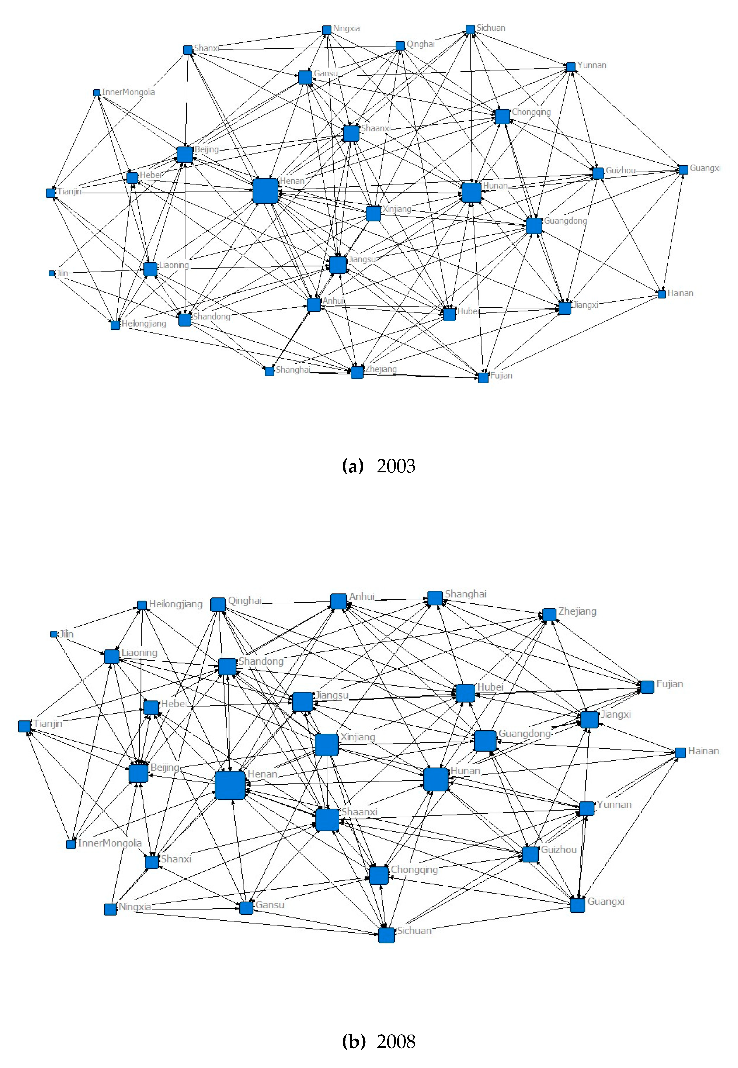
To capture overall structural characteristics of the spatial correlation network for China’s construction industry, we calculated carbon emissions connection values between different provinces on the base of the modified gravity model and established the inter-provincial correlation matrix after the binary process. Next, binary correlation matrixes were imported into the NetDraw, a tool of visualization in UNICET, to intuitively exhibit the spatial correlation status of the Chinese regional CO₂ emissions network for construction, and the network maps of every five years (2003, 2008, and 2017) were presented to show the evolution rules (see Figure 1). In the figure, the scale of the nodes represents the number of radiation connections they have, that is, the bigger the node is, the more regions it radiates. It should be noted that arrows indicate a significant transfer of construction carbon emissions from one province to another, while the absence of arrows and sides indicates no significant spatial transfer of construction carbon emissions between the two provinces. From that, we can see intuitively that the structure of spatial association presents a typical network morphology.

As shown in Figure 1, in 2003, the spatial association of China’s construction industry showed an obvious “core-periphery” network structure, with Henan, Jiangsu, Hunan, and Guangdong as the network center and the rest of the provinces generally at the edge of the network. The overall distribution of carbon emissions association was unbalanced. However, the distribution of network associations became more even in its evolution from 2008 to 2017, as more provinces shifted from the periphery to the center, and fewer provinces became marginal. The network includes 215 associations within 30 provinces, and several spatial associations exist in each province, indicating a typical spatial association of CO₂ emissions in each province of China’s construction industry and the existence of a stable spatial association structure.

It can be seen from Figure 2 that network efficiency has shown a certain cyclical change, with rapid growth from 2003 to 2009, an upward trend from 2012 to 2014, and a significant decline in 2010–2012 and 2015–2017. This result indicates that interprovincial network connectivity first tended to fluctuate and weaken, and after 2014, it tended to strengthen and stabilize. Moreover, these cyclical characteristics are opposite to the evolution of network density during the same period. The decline in network density, and the increase in network efficiency in the previous period can be attributed to the unbalanced regional development of infrastructure and residential construction and the outflow of labor from the backward to the developed regions. However, under the impact of government policies to strengthen infrastructure construction in backward regions and balanced regional economic development, high and low inflection points in network density and network efficiency were observed in 2014, respectively. From the perspective of national policies, China has proposed strategies to promote the rise of the central region and the development of the western region during the 11th and the 12th Five-Year Plans. Furthermore, to answer the international financial crisis in 2008, a “four trillion yuan” stimulus program was launched by the Chinese government, and a substantial amount was invested in infrastructure construction. The introduction of these policies has promoted balanced regional economic development and accelerated the urbanization of the undeveloped regions as well as the return of labor. As a result, network density and efficiency of the spatial correlation network exhibit certain cyclical features.

The calculation results indicate that network connectedness and hierarchy were 1 and 0.2598, respectively, from 2003 to 2017. When the importance of network connectivity is 1, according to Scott (2007) [40], it means that the two provinces in the network can establish spatial connections directly or indirectly, such that there are no independent entities within the network, so that the whole network has a significant spatial association effect. Moreover, network hierarchy has remained the same, suggesting that the hierarchy of spatial associations has not changed significantly.

4.2. Centrality Analysis

According to the method in Section 3, we consider each province to be a social actor in order to measure the “power” of nodes in a network from a “relation” perspective and analyze their capacity to regulate and manipulate other actors in terms of degree centrality, betweenness centrality, and closeness centrality. With the average of original data from 2003 to 2017, we calculated each kind of centrality index for the Chinese regional construction CO₂ emissions spatial association network. The distributions of the centrality indices are displayed in Figure 3.

Figure 3a shows that the regions in the first-degree centrality gradient are primarily located in central and eastern China, specifically Jiangsu, Henan, Hubei, Hunan, Guangdong, and Beijing, as well as the western provinces Xinjiang and Shaanxi. The reasons may be related to the fact that central and eastern provinces have a superior economic base, high technical level, and advantageous location conditions. However, the number of receiving relationships in Xinjiang is much lower than the number of sending relationships, indicating its stronger dependence on other provinces, and its carbon spatial correlation with other regions is mainly due to its rapid development and increasing energy consumption level in recent years, which is consistent with the conclusion of Yang and Chen (2019) [44]. For another, the provinces in the fourth-degree centrality gradient are Heilongjiang, Jilin, Inner Mongolia, and Hainan, mostly sited on the periphery of the geographical range in China with fewer associations with other regions.

Betweenness centrality measures the extent to which a point is located in the middle of the connection between two other points in the network; if a point has a greater degree of betweenness centrality, it is likely to play an important “bridge” role and is therefore at the center of the network. The average betweenness centrality of the 30 provinces was 4.536, with a sum of 136.085. The above-average provinces included Shaanxi, Shanxi, Hebei, Henan, Anhui, Liaoning, Inner Mongolia, and Guangdong (see Figure 3b). According to the National Bureau of Statistics of China, by 2017, the population of Henan was 95.59 million, ranking the third in China. The development standard of its economy, however, is comparatively backward. For the year 2017, the per capita GDP of Henan was 46,674 yuan/person, ranking 19th in China. However, its adequate workforce does not balance its degree of economic growth. Meanwhile, located in the western region center, Shaanxi’s population mobility is also very high. Hebei, Shanxi, and Anhui export a large amount of labor to the Beijing-Tianjin-Hebei region and the Yangtze River Delta region. The massive population migration necessarily brings about a growth in construction carbon emissions and underlines these regions’ central role among the network of spatial correlation. It should be mentioned that the energy intensity for the construction industry of Inner Mongolia was 3.24 in 2017, while no other provinces exceeded 1. The backwardness of the technical level in the construction sector and the large consumption of energy are the reasons for the high betweenness centrality of Inner Mongolia in the carbon emissions association network.

Closeness centrality is a measure that represents the reachability of a node with other network nodes. If a point has a high overall centrality, its distance from all other points in the networks is short. As seen from Figure 3c, the closeness centrality of Henan, Jiangsu, Hunan, Guangdong, Shaanxi, and Xinjiang is higher than the average and is situated on the first gradient. Most of these provinces have a high demand for construction and a high level of construction industry development. The exponential expansion of industry, the rise in people’s housing needs, and the heavy use of coal and other resources have contributed to severe carbon emissions. Xinjiang also showed remarkable spatial correlation characteristics, at which time its closeness centrality was higher than the surrounding provinces. This appearance has a close connection with economic growth, development of resources, and industrialization of Xinjiang [44].

4.3. Influencing Factors Analysis by QAP

For this article, 5000 random permutations were chosen to acquire the spatial correlation coefficient between the spatial correlation matrix of the construction industry and the driving factors with the UCINET software, as shown in

Table 3. Results of quadratic assignment protocol (QAP) correlation analysis.

	Coefficient	Significance	Average	Std Dev	Minimum	Maximum
Geographical Adjacency	0.492 ***	0.000	0.001	0.042	−0.148	0.153
Difference in Economic Development	−0.022	0.310	0.000	0.045	−0.205	0.146
Difference in Energy Intensity	−0.081 **	0.042	0.000	0.046	−0.162	0.151
Difference in Industrial structure	−0.120 ***	0.005	0.000	0.043	−0.163	0.132
Difference in Industrial agglomeration	−0.077 **	0.048	0.000	0.044	−0.190	0.143
Difference in Environmental Regulation Intensity	−0.069 *	0.068	0.000	0.047	−0.187	0.146

Notes: *** Significance at 1% level; ** Significance at 5% level; * Significance at 10% level.

. “Average” and “Std. Dev” represent the mean value and the standard deviation of the coefficients for 5000 permutations. “Minimum” and “Maximum” are the minimum and the maximum values of the coefficients, respectively. Furthermore, “Prop ≥ 0” denotes the probability that all coefficients obtained by the matrix permutation are greater than or equal to the actual coefficient, whereas “Prop ≤ 0” suggests the reverse probability. At the 1% level, the correlation coefficient between geographic adjacency and the matrix of spatial relationships is highly positive, meaning that they have a positive correlation. The correlation coefficient between the difference in industrial structure and the spatial correlation is substantially negative at the 1% level. At the 5% level, the correlation coefficients between energy intensity differences and industrial agglomeration differences and spatial correlations are all significantly negatively correlated. The correlation coefficients between environmental regulation intensity differences and spatial correlation are significant at the 10% level and are negative. The interprovincial differences in economic development did not pass the significance test, indicating that the variable is not correlated with spatial correlation. The above results are based only on correlation analysis, and the QAP regression analysis should be applied to verify the preliminary results.

The purpose of QAP regression analysis in this paper is to study the regression relationship between multiple influence factor matrices and the spatial correlation matrix. Based on the QAP correlation results, this study removes the variable of difference in economic development and chooses the remaining six influencing factors with remarkable coefficients as the independent variables for QAP regression analysis. The results of the data randomly permuted 2000 times calculated from UCINET are shown in

Table 4. Results of QAP regression analysis.

Independent	Unstandardized Coefficient	Standardized Coefficient	Significance	Proportion as Large	Proportion as Small
Geographical Adjacency	0.595	0.489 ***	0.001	0.001	1.000
Difference in Energy Intensity	−0.055	−0.054 *	0.087	0.914	0.086
Difference in Industrial structure	−0.057	−0.066 **	0.042	0.958	0.042
Difference in Industrial agglomeration	−0.004	−0.005	0.426	0.574	0.426
Difference in Environmental Regulation Intensity	−0.011	−0.012	0.365	0.635	0.365
Intercept	0.159	0.000	-	-	-

Notes: *** Significance at 1% level; ** Significance at 5% level; * Significance at 10% level.

.

In Table 4, “Proportion as large” conveys that the absolute value of the random replacement determination coefficient is not less than the determination coefficient observed, and “Proportion as small” describes that the absolute value of the determination coefficient generated by stochastic replacement is not greater than the obtained determination coefficient. The outcomes indicate that the geographical adjacency and the differences in industrial structure and in energy intensity have significant effects on the spatial correlation network formation. The coefficient of the geographical adjacency matrix is strongly positive at the 1% level, suggesting that the geographical adjacency assumes a crucial role in the development of the spatial correlation network. The explanation for this is because business contact as well as resource transport between geographically neighboring provinces are more common, reinforcing the spatial connection. However, the differences in industrial structure and energy intensity are significantly negatively correlated at the levels of 5% and 10%, respectively, indicating that the differences in industrial development level and energy saving technologies in the construction industry in different regions are not conducive to the formation of spatial associations. The differences in the industrial agglomeration and the environmental regulation intensity are not significant, suggesting that differences in the degree of agglomeration and environmental policy management in the Chinese construction sector do not have a significant impact on the formation of a spatial association network of carbon emissions from the construction industry.

5. Discussion

This paper provides a new perspective on the spatial analysis of carbon emissions of the inter-provincial construction industry in China. First, using the gravity model, this study overcomes the limitation of the time lag of the traditional VAR model and can analyze the evolutionary characteristics of the network structure through cross-sectional data, while the modified gravity model takes into account the geographical adjacency and the main factors affecting construction emissions (carbon emission scale, population scale, and economic level) and is more able to reflect the spatial characteristics of construction emissions. Bai et al. (2020) verified the reliability of the modified gravity model by demonstrating the significant correlation between the modified carbon emission spatial association matrix and the related variables in the analysis of the spatial correlation data over the years [26]. Yang and Liu (2020) studied the spatial association of low carbon innovation in China by using a modified gravity model through the analysis of manufacturing patents data [36]. In this paper, a construction carbon emission network was constructed by constructing a spatial correlation matrix obtained from a modified gravity model. Second, in the analysis of the overall structure and the characteristics of the spatial association networks, the SNA also has advantages over traditional measurement methods, which can visually present the structural state of the spatial association networks, and the characteristics of both individuals and the whole in the network can be detected [37]. This paper constructed a spatial association network as the object of social network research through a modified gravity model, which can intuitively and completely analyze the evolution pattern of inter-provincial construction carbon emission network characteristics in China. Third, the QAP method can overcome the problems of multicollinearity and autocorrelation, thus this paper applied this method to correlation as well as regression analysis of the factors influencing the spatial association of carbon emissions in the construction industry and obtained similar conclusions as Lu et al. (2020) [17], that is, inter-provincial carbon emissions in the Chinese construction industry have significant spatial correlation characteristics, and spatial adjacency, energy intensity, and industrial structure have significant effects on them.

Moreover, the result of network density and efficiency shows that the closeness degree of spatial correlations tended to increase, with a high and a low inflection point for network density and network efficiency, respectively, and network connections tended to stabilize in 2014. This result is also reasonable considering that the global economic crisis in 2008 and the economic development afterward made the construction carbon emissions decrease and then increase. Lu et al. (2020) [17] and Du et al. (2018) [28] have come to a similar conclusion. According to the findings of the QAP regression, it can be found that the spatial association of CO₂ emissions for the construction sector would be significantly influenced by geographical adjacency and the differences in energy intensity and industrial structure. Qin et al. (2019) [22] and Yang and Liu (2020) [36] showed that geographical proximity is the main factor of spatial relationships, and industrial structure, technology level, and other factors also significantly affect spatial correlation.

6. Conclusions and Policy Recommendations

This paper used SNA to analyze the structural characteristics and the influencing factors of the spatial network for the Chinese construction industry. A modified gravity model was utilized to build up the interprovincial carbon emissions spatial association matrix and discover the overall characteristics and the centrality characteristics of the spatial correlation network based on this matrix. Finally, QAP correlation analysis and regression analysis were applied to investigate the ingredients impacting the spatial correlation of carbon emissions for the construction sector. The conclusions and the policy recommendations were drawn based on the results of the above analyses.

First, as network efficiency shifted from cyclical fluctuations to an overall downward trend, network connections tended to strengthen and stabilize after 2014. The connectedness and the hierarchy of the network, however, were invariably 1 and 0.2598, respectively. In general, the spatial association’s closeness degree indicated a growing pattern, and network connections appeared to be more stable. The intuitive spatial correlation network structure of the Chinese inter-provincial construction industry’s CO₂ emissions implies that the Chinese government should pay attention to the spatial CO₂ emissions correlation in the inter-provincial construction sector and introduce coordinated cross-regional governance.

Second, from the degree centrality results, it can be concluded that the central region (Henan, Hubei, Hunan, Shaanxi), the developed regions (Beijing, Guangdong, Jiangsu), and Xinjiang have a high level of provincial construction carbon emissions association; regional synergistic emission reduction can be carried out by adjusting the energy structure, improving industry emission reduction standards, and carrying out market interventions in these regions. The result of the betweenness centrality shows that the regions above the average are Henan, Anhui, Shaanxi, Shanxi, Hebei, Guangdong, Liaoning, and Inner Mongolia, etc., and the spatial carbon emissions of the construction industry can be controlled by improving the industrial structure and the energy efficiency in these regions. The results of closeness centrality indicate that regions with closer connections to other provinces are mainly concentrated in regions with higher levels of construction industry development (Henan, Jiangsu, Hunan, Guangdong, Shaanxi, and Xinjiang). For these regions, the transmission flow of carbon emissions from the construction industry in the network can be enhanced through market cooperation and the establishment of regional development mechanisms.

Third, QAP regression analysis indicates that the reduction of industrial structure and energy intensity differences can significantly facilitate the spatial association of carbon emissions for the construction industry. Therefore, the Chinese government should put forward a reasonable development program for the construction industry to continuously reduce the differences in the industrial structure and the energy intensity of the construction industry within various provinces. Specifically, the government can increase investment in infrastructure construction in backward regions, promote low-carbon development in the construction industry, encourage technological upgrading and innovation in less developed regions, as well as introduce high-tech enterprises through preferential policies so that the industrial structure can be optimized and energy intensity can be reduced, thus narrowing the gap between them and developed regions.