Identify Optimal Traffic Condition and Speed Limit for Hard Shoulder Running Strategy

Abstract

Highway system is experiencing increasing traffic congestion with fast-growing number of vehicles in metropolitan areas. Implementing traffic management strategies such as utilizing the hard shoulder as an extra lane could increase highway capacity without extra construction work. This paper presents a method of determining an optimal traffic condition and speed limit of opening hard shoulder. Firstly, the traffic states are clustered using K-Means, mean shift, agglomerative and spectral clustering methods, and the optimal clustering algorithm is selected using indexes including the silhouette score, Davies-Bouldin Index and Caliski-Harabaz Score. The results suggested that the clustering effect of using K-Means method with three categories is optimal. Then, cellular automata model is used to simulate traffic conditions before and after the hard shoulder running strategy is applied. The parameters of the model, including the probabilities of random deceleration, slow start and lane change, are calibrated using real traffic data. Four indicators including the traffic volume, the average speed, the variance of speed, and the travel time of emergency rescue vehicles during traffic accident obtained using the cellular automata model are used to evaluate various hard shoulder running strategies. By using factor analysis and TOPSIS (Technique for Order Preference by Similarity to Ideal Solution) methods, the optimal traffic condition and speed limit of opening hard shoulder could be determined. This method could be applied to highway segments of various number of lanes and different speed limits to optimize the hard shoulder running strategy for highway management.

1. Introduction

With the development of economy, the highway system become increasingly overloaded with traffic. The excessive traffic load induced increasing frequency of traffic congestion and incidents, especially during holidays. The problem of traffic congestion has affected people’s quality of life and caused economic losses. It has been reported that the economic loss of travel time delay and fuel consumption was $121 billion in 2011 worldwide [1,2], and the annual loss was estimated to reach $199 billion in 2020 [3]. Construction of new highways would cost huge funding budget and require long construction period. In addition, the growth rate of new highway mileages is far less than the growth rate of traffic volumes. Therefore, the more effective way to relieve the traffic congestion on highway is to use appropriate transportation management techniques to maximize the operating efficiency of current transportation facilities compared with expanding more highway mileages.

Recently the Active Traffic Management System (ATMS) has aroused wide attention of researchers and engineers. The effective approaches of the ATMS include the Advisory Variable Speed Limits (AVSLs), Lane-Use Control Signals (LUCS) and Dynamic Hard Shoulder Running. One research studied the effects of the three approaches and found that most of the improvements occurred in the hard shoulder running section [4]. A typical hard shoulder has a width of more than three meters and is usually placed on the right side of the road which can meet the parking and driving need of vehicles. In most countries the hard shoulder is used as an emergency lane which allow drivers to stop and handle emergency events, however running on the emergency lane is generally prohibited for safety concerns. Some countries started to use the hard shoulder as an extra running lane to alleviate traffic congestion on highway [5,6,7]. Germany has used hard shoulder to evacuate traffic flow since 1996 [8,9]. In Netherlands, bus was allowed to operate on the hard shoulder, and hard shoulder running has been implemented on around 1000 km of highway segments since 2003 [8]. It was found that using the hard shoulder as additional travel lane led to a saving of 50,000 Euros per day in Germany, and a reduction in the overall fuel consumption by 4% was measured in England [10]. One research estimated that when the hard shoulder was opened, congestion frequency fell by between 68% and 82%, and average speed (same traffic volume) rose by 9% [11]. Another research suggested that using hard shoulder as additional travel lanes would not induce adverse changes and some countries even found decreases in accidents associated with opening hard shoulder [10]. Therefore, as can be induced from previous experiences, if the safety factors could be properly managed, opening the hard shoulder have great potential in increasing traffic capacity of highways.

Various studies have been conducted in investigating proper methods to utilize the hard shoulder for normal vehicle operation [12]. Farrag et al. [13] evaluated the impacts of hard shoulder running strategy and ramp closure strategy using a simulation-based method with the Vissim software. Berger and Maurer [14] conducted a cost-benefit analysis to identify what traffic volume range is economically advisable to permit hard shoulder running. The cost includes the investment cost, maintenance cost, user’s cost (travel time and operating cost), environmental damage cost and accidents cost. Bergmeister et.al [15] utilized the speed of the traffic flow to determine the opening and closing of the hard shoulder. Zhou.et.al [16] used Q-learning method to coordinate hard shoulder running control strategy to optimize the travel time. Karan [17] proposed a dynamic control strategy of opening hard shoulder using variable speed limit. In conclusion, the previous researches could be improved in three aspects: (1) Previous researches mainly relied on single traffic parameter such as the traffic volume or the speed to determine the proper condition to permit hard shoulder running. However, it’s not accurate to represent the traffic condition purely depend on one single traffic parameter. A comprehensive standard could be established to evaluate various traffic conditions. (2) Many of the previous researches focused on improving the traffic efficiency, however as indicated by Kellerman [11], when the hard shoulder lane was opened, the possibility of lane changing would increase, which may result in rear end collisions. Therefore, when optimizing hard shoulder running strategy, both efficiency factors and safety factors should be considered. (3) Few studies have mentioned how to set the optimal speed limit of the hard shoulder lane. When applying hard shoulder running strategy, the speed limit should be set properly to optimize both traffic efficiency and travel safety.

This paper aims to identify proper traffic condition to open hard shoulder as an extra lane and to optimize the speed limit of the hard shoulder lane. The rest of the paper is organized as follows: Section 2 introduces the data used in this research; Section 3 introduced the methodology, which includes three parts: methods of clustering traffic states, traffic simulation method using cellular automata model, and optimization method for determining optimal traffic condition and speed limit. Section 4 presents the results, and the conclusions and discussions are introduced in the final section.

2. Research Data

The traffic data used in this research is collected in the Shanghai-Nanjing expressway, which is a tier 1 level expressway that connects two major metropolitan areas of China. This expressway was built in 1996, which has four lanes in each direction and each lane is 3.5 m in width. Hard isolation is used to separate opposite driving directions in this highway segment. The width of the central separation belt is 4.5 m. In each direction, there is hard shoulder with the width of 3.25 m. The current speed limits on the four-lane highway segment is 120 km/h, 120 km/h, 100 km/h, 100 km/h respectively. The cross-section design and the speed limit configuration followed the regulations of the Ministry of Transport of China. In 2015, this regulation is updated which require that the lane width for the new expressways should be 3.75 m and the hard shoulder should be 3.5 m in width. Therefore, for both of the existing expressways and new expressways, the difference of the widths between the normal driving lanes and the hard shoulder is not significant, and the width of the hard shoulder is sufficient for traffic operation.

Millimeter-wave radar sensors are installed along both directions of the highway, which could collect traffic data include the traffic counts and the vehicles’ speed simultaneously from the four lanes every 30 s. These traffic data are aggregated by 5 minutes’ interval in order to facilitates further analysis. The traffic data used in this research are collected from May 1 to May 4 in 2019, which is during national holiday period. In this four-day long holiday, tolling fee is free for all types of vehicles. Compared with normal days, the traffic volume and chances of traffic incidents are higher in the tolling-free holidays. We select the traffic data in this period in order to simulate more complex traffic conditions. The data is used to calibrate the parameters of the cellular automata model.

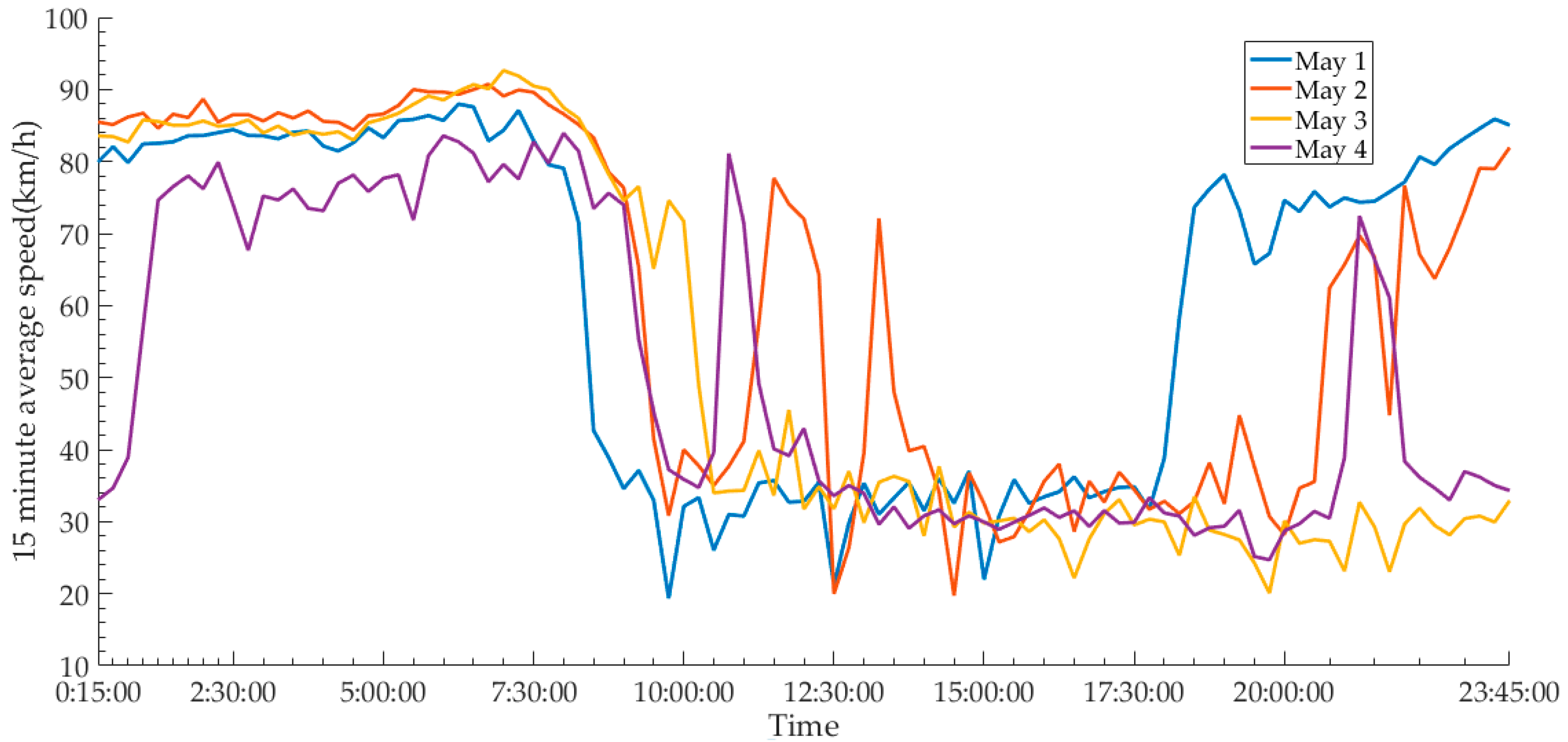
Figure 1 presents the variation of traffic volume and Figure 2 presents the average speed of the road segment during the research period. On May 1, from 8:30:00 to 17:30:00, it was apparent that the average speed was lower and the traffic volume was higher. On May 2, from 9:00:00 to 14:30:00, the fluctuation of traffic volume and average speed was comparatively large. From 14:30:00 to 20:00:00, it could be seen that traffic volume was higher and average speed was lower. On May 3 and May 4, the traffic volume was higher and the average speed was lower from 12:00:00 to 23:55:00. However, the fluctuation of traffic volume on May 4 was larger than May3. At about 9:30:00 in May 4 and 14:00:00 in May 2, the average traffic volume was the highest, with approximately 1800 vehicles/hour/lane. At about 9:30:00 in May 1, 12:30:00 in May 2 and 14:30:00 in May 2, the average speed was the smallest, with approximately 15 km/h. The reasons may be that May 1 was the first day of the vacation and May 4 was the last day of the vacation.

Figure 3 and Figure 4 displays the distribution of the hourly traffic volume and hourly average speeds on each of the four lanes. The lane next to the center belt is numbered as lane 1, and the lane adjacent to the hard shoulder is numbered as lane 4. As can be seen in Figure 1, the average volume generally decreases from lane 1 to lane 4. The peak hour starts at 8:00 on lane 1 and lane 2, while on lane 3 and lane 4, the peak hour starts from 9:00. The traffic volume is relatively low in the period from 1:00 to 7:00. Figure 4 indicates that in the non-peak hours from 1:00 to 7:00, the average speed on each lane is about 100 km/h, 90 km/h, 80 km/h, 70 km/h from lane 1 to lane 4 respectively. The traffic volume distribution and the average speed distribution can be attributed to the speed limits of the lanes. The speed limit on lane 1 and lane 2 is 120 km/h, and the speed limit on lane 3 and lane 4 is 100 km/h. Most of the small vehicles would drive on lane 1 and lane 2 while most of the heavy vehicles would operate on lane 3 and lane 4. We can find an obvious decrease of the average speed from 10:00, and the average speed starts to increase at about 19:00. The speed variations are comparatively large from 19:00 to 24:00. The average speeds are always very low from 13:00 to 18:00, with about 40 km/h on the first two lanes and 30 km/h on the last two lanes.

3. Methods

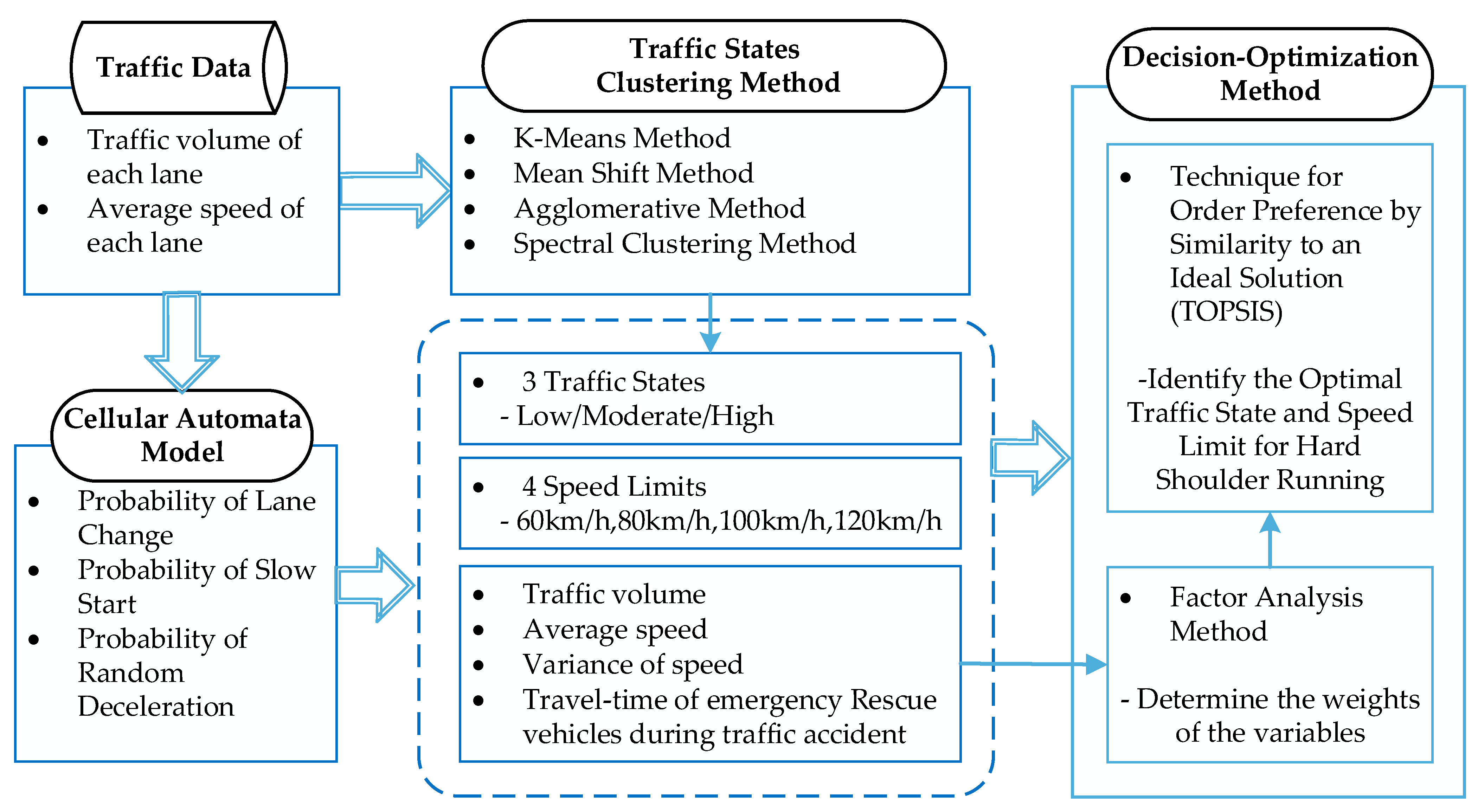
The methodology could be divided into three parts, including the traffic states classification using clustering methods, the traffic simulation using cellular automata model and the decision-optimization methods for identifying optimal traffic states and speed limit, respectively. Figure 5 presents the flow chart of the methodology. (a) Firstly, we used several clustering methods to group similar traffic states. The traffic state varies with different time-of-day and different day-of-week, different traffic management strategies could be applied to different traffic states in order to achieve higher traffic efficiency. However, there’s no uniform indicator to quantify the traffic states of highway. In order to simply the solution, we firstly used clustering methods to group similar traffic patterns together based on the traffic volume and the average speed on each lane. (b) Secondly, the cellular automata model is used to simulate varies traffic scenarios, including the traffic condition after the hard shoulder is used as an extra lane under various speed limits and the traffic condition when traffic accident happened. The parameters of the cellular automata model, including the probabilities of the lane change, slow start, and random deceleration behavior, are calibrated using the real world data as introduced in the previous section. By using the cellular automata simulation model, we can obtain four traffic parameters including the traffic volume, the average speed, the variance of the speed and the travel time of emergency rescue vehicles. (c) Finally in the decision optimization part, we used factor analysis method to determine the weight of the four traffic parameters obtained from the cellular automata model, and then the Technique for Order Preference by Similarity to an Ideal Solution (TOPSIS) method is used to identify the optimal traffic state and speed limit of opening hard shoulder.

3.1. Clustering Traffic States

Nowadays with the wide spread of electronic sensors equipped on highways, such as loop coil, video detector, ultrasonic detector and etc., it is easy to obtain traffic parameters such as speed, time occupancy, traffic volume, time-headway and etc. All of them could reflect traffic states. However there’s no uniform indicator to quantify the level of congestion of highway [18,19]. Low traffic volume could indicate two contradictory conditions. For example, when the number of vehicles on the road is few, drivers can drive at the high speed limit; when the number of vehicles on the road is very high, conflictions between vehicles would increase and the frequency of stopping and starting would also increase, which result in low average speed and low traffic volume. Therefore, classifying traffic states should consider more than one traffic flow parameter. This paper selected indications of the average speed and the traffic volume of each lane to cluster the traffic states.

There are various clustering models, such as K-means, mean shift, agglomerative clustering, spectral clustering and etc. The K-means method is one of the most popular and simplest clustering method [20]; the mean shift method is a centroid-based algorithm with the aim of discovering blobs in a smooth density of samples [21]; the spectral clustering method is based on graph theory [22]; the agglomerative clustering method is based on hierarchical methods with the main idea that each observation started in its own cluster, and clusters are successively merged together [23]. Therefore, it is difficult to choose an optimal clustering algorithm to cluster traffic states.

The purpose of clustering is to ensure that the differences in the same traffic state cluster are small and the differences in different traffic state clusters are large. Silhouette Score, Davies-Bould in Index and Caliski-Harabaz Score are chosen to evaluate the effect of the clustering methods.

Silhouette score can be calculated by the following equation:

$$\mathrm{s}=\frac{b-a}{\max \left(a,b\right)}$$

(1)

where $a$ is the average distance between the sample and all points at the same cluster, b is the average distance between the sample and the closest cluster of all points.

The range of silhouette score is from −1 to 1. When the silhouette score is closed to 1, it means that the sample is similar to all points at the same cluster, and the sample is not similar to other points at other clusters. Higher silhouette score indicates better clustering effect.

Davies-Bouldin Index can be calculated by the following equation:

$$\mathrm{DBI}=\frac{1}{N}\ast {\displaystyle \sum }_{i=1}^{n}MA{X}_{i\ne j}\left(\frac{a_i+a_j}{d\left(c_i,c_j\right)}\right)$$

(2)

where: $d\left(c_i,c_j\right)$ is the distance between centers of clusters; $a_i$ is the average distance between the center and all points at the same cluster. N is the number of clusters. When the Davies-Bouldin Index is small, it indicates that the effect of clustering is good.

Caliski-Harabaz Score can be calculated by the following equation:

$$\mathrm{c}=\frac{M-K}{K-1}\ast \frac{T_r\left(B_k\right)}{T_r\left(W_k\right)}$$

(3)

where:$M$ is the number of samples, K is the number of clusters, $T_r\left(B_k\right)$ is the trace of covariance matrix of different clusters, $T_r\left(W_k\right)$ is the trace of covariance matrix of the same clusters. When Caliski-Harabaz Score is large, it represents that the effect of clustering is good.

3.2. Cellular Automata Model

The cellular automata model is a simulation model based on discrete space, time and states, and it’s suitable for fast computer calculations [24]. A cellular automata comprises a regular grid of cells, each cell can only take finite states, and the rules of states updating should be local and synchronous [25]. State updating of each cell is only related to its own state and the states of the surrounding cells. Each cell follows the same rule of updating according to the states of the neighborhood cells and its own state [26]. This process is similar with actual vehicles running and therefore the cellular automata model is frequently used in traffic simulation. In addition, the mechanism of the cellular automata model ensured that error accumulation won’t happen in the process of simulation, and the accuracy of the simulation would be sufficient to be used in long-time simulation.

This research utilized cellular automata model to obtain the traffic volume, average speed, time-headway and travel time of emergency rescue vehicles during traffic accident. As the research highway segment have four running lanes and one emergency lane (hard shoulder), five rows of cellular automata cells are built with 1000 cells in each row. The length of each cell is set as 50/9 m. Two different types of cell spacing are used, which includes the ordinary lane cell spacing and hard shoulder cell spacing. The cellular automata adopted the periodical boundary in simulation. The cells have three cell states: 0 represents that the cell is NOT occupied, 1 represents the cell is occupied, −1 represents the cell is impassable. In reality, the speed limit of each lane is 120 km/h, 120 km/h, 100 km/h, and 100 km/h from the first lane to the fourth lane respectively. Therefore, in cellular automata model, the speed limit of each lane is set as 6 cells/s, 6 cells/s, 5 cells/s, and 5 cells/s respectively. The hard shoulder did not have speed limit. However, from the perceptive of safety, when the hard shoulder is opened, all vehicles in the hard shoulder should obey speed limit rule. Therefore, it is meaningful to study optimal traffic states of opening hard shoulder and the speed limits for the hard shoulder. The original function of the hard shoulder lane is to serve as an emergency lane for emergency rescue vehicles to bypass traffic jams to get to the accident location or as a temporary safe parking place for malfunctional vehicles. It’s necessary to compare traffic condition with the influence of traffic accidents before and after the hard shoulder is opened. The length of accident area is set as 30 cells, which equals to 500/3 m.

This research utilized cellular automata model to obtain the traffic volume, average speed, time-headway and travel time of emergency rescue vehicles during traffic accident. As the research highway segment have four running lanes and one emergency lane (hard shoulder), five rows of cellular automata cells are built with 1000 cells in each row. The length of each cell is set as 50/9 m. Two different types of cell spacing are used, which includes the ordinary lane cell spacing and hard shoulder cell spacing. The cellular automata adopted the periodical boundary in simulation. The cells have three cell states: 0 represents that the cell is NOT occupied, 1 represents the cell is occupied, −1 represents the cell is impassable. In reality, the speed limit of each lane is 120 km/h, 120 km/h, 100 km/h, and 100 km/h from the first lane to the fourth lane respectively. Therefore, in cellular automata model, the speed limit of each lane is set as 6 cells/s, 6 cells/s, 5 cells/s, and 5 cells/s respectively. The hard shoulder did not have speed limit. However, from the perceptive of safety, when the hard shoulder is opened, all vehicles in the hard shoulder should obey speed limit rule. Therefore, it is meaningful to study optimal traffic states of opening hard shoulder and the speed limits for the hard shoulder. The original function of the hard shoulder lane is to serve as an emergency lane for emergency rescue vehicles to bypass traffic jams to get to the accident location or as a temporary safe parking place for malfunctional vehicles. It’s necessary to compare traffic condition with the influence of traffic accidents before and after the hard shoulder is opened. The length of accident area is set as 30 cells, which equals to 500/3 m.

In this paper, we assumed five rules for cellular automata, which includes the acceleration, random deceleration, lane change, slow start and deceleration rule.

• Acceleration rule: $V_n\to \min \left(V_n+1,V_{max}\right)$. This rule described the drivers are expected to drive at the maximum speed.
• Random deceleration rule: with probability $P_1$, $V_n\to \max \left(V_n-1,0\right)$, the speed of vehicles would slow down due to various uncertain reasons.
• Lane change rule: with probability $P_2$, and , the vehicle would change the lane.
• Slow start rule: with probability $P_3$, and $V_n$= 0, instead of accelerating, the vehicle would keep the original position.
• Deceleration rule:$V_n\to \min \left(V_n,d_n\right)$. This rule described the measures taken by the driver to avoid a collision with other cars.

Where, $d_n$ is the number of cells between the vehicle and the vehicle in front on the same lane; $d_{n,other}$ is the number of cells between the vehicle and the vehicle in front on the target lane; $d_{n,back}$ is the number of cells between the vehicle and the vehicle behind on the target lane; $V_{max}$ is the speed limit of the lane; $V_n$ is the speed of the vehicle.

The cellular automata model is calibrated using the research data including the traffic volume and the average speed aggregated by 5 min interval. For each of the three traffic conditions, the corresponding set of model parameters $P_1,P_2,P_3$ are adjusted to minimize the RMSE (Root Mean Square Error) between the field data and the simulated data. The RMSE can be calculated as follows:

$$\mathrm{RMSE}=\sqrt{\frac{1}{n}\ast {\displaystyle \sum }_{i=1}^n{\left(y_i^{{}^{\prime }}-y_i\right)}^2}$$

(4)

where, $y_i^{{}^{\prime }}$ represents the value obtained by simulation, $y_i$ refers to the real value, n is the number of values. By comparing RMSE, better probabilities of $P_1,P_2,P_3$ could be selected.

3.3. Decision-Optimization Methods

After using cellular automata simulation models, we could obtain the traffic volume, average speed, variance of speed and travel time of emergency rescue vehicles during traffic accident. For better transportation service, we wish to maximize the traffic volume and the average speed to improve the traffic efficiency. However, for safety concerns, we need to minimize the variance of the speed, since large speed variance may lead to safety issues. We also concerned if accidents do happen, we need to use the hard shoulder as the emergency lane, and the travel time of the emergency rescue vehicle to the accident location should be minimized. In order to balance the multiple contradictory targets, we use factor analysis method in combination of TOPSIS method as the decision-optimization methods to determine an optimal traffic state and speed limit of opening hard shoulder.

Factor analysis is a multivariate statistical analysis method, which is based on the study of the internal dependencies of variables, and some variables with complex relationships are reduced into a few comprehensive factors [27,28]. The original variables are expressed and processed through linear combination [29]. The specific steps of factor analysis include: calculating the correlation coefficient matrix and selecting the main factors based on eigenvalues, calculating the rotated matrix by the maximum variance method, and obtaining weight of indicators with the adoption of contribution rate. The rate of contribution can be calculated as followed:

$$b_j=\frac{{\lambda }_j}{{{\displaystyle \sum }}_{k=1}^m{\lambda }_k} \mathrm{j} = 1, 2, 3, \dots , \mathrm{m}$$

(5)

where ${\lambda }_j$ is eigenvalue, $b_j$ is rate of contribution, $y_j$ is the value of new comprehensive index. Higher comprehensive score indicates better scheme.

TOPSIS (Technique of Order Preference Similarity to the Ideal Solution) is a useful technique in dealing with multi-attributes or multi-criteria decision making problems [30]. It could help decision makers carry out analysis, comparisons and ranking of the alternatives [31]. The TOPSIS method first construct positive ideal solutions and negative ideal solutions of the decision-optimization problems, then calculate the distance between each scheme and the positive ideal solution and the negative ideal solution for comparisons [32]. The computation process of the TOPSIS method is straightforward and easy to implement [33]. In addition, the decision process permits the pursuit of best alternatives for each criterion depicted in a simple mathematical form [33]. The reason of both positive ideal solutions and negative ideal solutions are used is that, when only positive ideal solution is used, sometimes two schemes may have the same distance between the positive ideal solution. In order to distinguish the pros and cons of the two schemes, it is necessary to use both positive ideal solutions and negative ideal solutions.

The distance between each scheme and the positive ideal solution is calculated as followed:

$$s_i^{*}=\sqrt{{{\displaystyle \sum }}_{j=1}^n{(C_{ij-}{C}_j^{*})}^2}, \mathrm{i} = 1, 2, 3, \dots , \mathrm{m}$$

(6)

The distance between each scheme and the negative ideal solution is calculated as followed:

$$s_i^0=\sqrt{{{\displaystyle \sum }}_{j=1}^n{(C_{ij-}{C}_j^0)}^2}, \mathrm{i} = 1, 2, 3, \dots , \mathrm{m}$$

(7)

Finally, an optimal scheme is selected by the following equation:

$$f_i^{*}=\raisebox{1ex}{$s_i^0$}\!\left/ \!\raisebox{-1ex}{$(s_i^0+s_i^{*})$}\right., \mathrm{i} = 1, 2, 3, \dots , \mathrm{m}$$

(8)

where: $C_j^{*}$ is the positive ideal solution, $C_j^0$ is the negative ideal solution. When $f_i^{*}$ is higher, it means that the scheme is better.

4. Results

This section describes the result of applying our methodology to identify the optimal traffic condition and speed limit for hard shoulder running strategy on the research highway segment. Section 4.1 compares the effects of several traffic states clustering method. Section 4.2 presents the results of traffic simulation using the cellular automata model and validates the model by comparisons between the simulated data with the field data. In Section 4.3, the cellular automata model is applied to obtain variables including the traffic volume, average speed, variance of speed and the travel time of emergency rescue vehicles during traffic accidents, before and after the opening of the hard shoulder. Section 4.4 compares various hard shoulder running scenarios under different traffic conditions and speed limits, and presents the result of the decision optimization method.

4.1. Results of Clustering Traffic States

In this paper, four clustering methods including the K-means method, the mean shift method, the agglomerative clustering method and the spectral clustering method are used to group similar traffic states. Silhouette score, Caliski-Harabaz Score and Davies-Bouldin Index are used to evaluate and select the optimal clustering algorithm. Higher value of silhouette score and Caliski-Harabaz Score lower value of Davies-Bouldin Index represents better clustering effect.

Table 1. Silhouette score, Caliski-Harabaz Score and DBI of K-means algorithm.

Cluster Number	Silhouette Score (K-Means)	DBI (K-Means)	Caliski-Harabaz Score (K-Means)
2	0.6046	0.6012	4824.4674
3	0.6014	0.5814	6235.6981
4	0.4484	0.7787	5554.2090
5	0.4253	0.8242	5925.4492
6	0.4202	0.8200	5826.7358
7	0.3946	0.8727	5920.5752
8	0.3713	0.8955	5712.3713
9	0.3361	0.9454	5578.5043

,

Table 2. Silhouette score, Caliski-Harabaz Score and DBI of Agglomerative algorithm.

Cluster Number	Silhouette Score (Agglomerative)	DBI (Agglomerative)	Caliski-Harabaz Score (Agglomerative)
2	0.6037	0.5998	4584.4790
3	0.5935	0.5735	5786.7530
4	0.5345	0.7359	5200.3829
5	0.4622	0.7560	5384.5324
6	0.4308	0.7848	5197.1510
7	0.3944	0.8863	5060.2791
8	0.3263	0.9981	4972.6302
9	0.3056	0.9902	5014.4874

,

Table 3. Silhouette score, Caliski-Harabaz Score and DBI of Spectral clustering algorithm.

Cluster Number	Silhouette Score (Spectral Clustering)	DBI (Spectral Clustering)	Caliski-Harabaz Score (Spectral Clustering)
2	0.6034	0.6000	4566.6627
3	0.6010	0.5813	6190.4380
4	0.5483	0.7000	5458.8068
5	0.4908	0.6659	5314.5480
6	0.4608	0.7511	5033.8106
7	0.3963	0.8103	5139.0803
8	0.3674	0.8488	4952.6232
9	0.3593	0.8641	4756.4975

and

Table 4. Silhouette score, Caliski-Harabaz Score and DBI of mean-shift algorithm.

KERRYPNX	Silhouette Score (Mean shift)	DBI (Mean shift)	Caliski-Harabaz Score (Mean shift)
0.5	0.1448	1.1194	1349.0838
0.8	0.3978	0.8621	4003.6231
1.1	0.5497	0.7003	5364.1282
1.4	0.5128	0.7454	5198.6654
1.7	0.5994	0.5731	6006.6977
2	0.6013	0.5787	6179.0463
2.3	0.6060	0.5992	4802.9241
2.6	0.6010	0.6048	4805.8280

record the silhouette score, Caliski-Harabaz Score and Davies-Bouldin Index of each clustering method.

By comparing data in Table 1, Table 2, Table 3 and Table 4, it’s obvious that the clustering effect is better under five conditions: K-means, spectral clustering and agglomerative algorithms with three categories, and mean-shift with bandwidth of 1.7 and 2 respectively. Therefore, in order to choose an optimal clustering algorithm, we also calculated the number of silhouette score less than or equal to 0, the number of silhouette score greater than average silhouette score, and the number of silhouette score greater than 0 and less than or equal to average silhouette score and showed in Figure 6.

As shown in Figure 6, when the K-means algorithm is adopted and the cluster number is 3, the number of silhouette score less than 0 is minimum and the number of other categories is maximum. When the silhouette score is negative, it means that the effect of some clusters is not good. The result indicated that the K-means algorithm performs better than the agglomerative, spectral clustering and mean-shift methods. Therefore, the K-means algorithm is adopted to cluster traffic states, and the traffic states would be grouped into three categories.

When the K-Means algorithm is adopted and the cluster number is three, in order to evaluate the clustering effect of each category, the silhouette score of each sample is plotted in Figure 7. In Figure 7, the red vertical line represents the average of the silhouette score of all samples. As Figure 7 presents, when the cluster label is 0 or 1, the number of samples with above-the-average silhouette score is larger, and there exists no sample with silhouette score less than 0. Therefore, for samples labeled 0 or 1, the effect of clustering is better.

Figure 8 illustrates the traffic states of each group. Cluster label 0 represents the high density group with corresponding density ranging from 140 pcu/km/four-lanes to 700 pcu/km/four-lanes, the range of 5 min traffic volume is from 270 pcu to 630 pcu, and the average speed is between 15 km/h and 55 km/h. Cluster label 1 represents low density group, the range of density is from 0 pcu/km/four-lanes to 50 pcu/km/four-lanes, the range of four-lanes-traffic volume of 5 min is from 65 pcu to 270 pcu, the average speed is between 75 km/h and 95 km/h. Cluster label 2 represents the moderate density group, the range of density is from 50 pcu/km/four-lanes to 140 pcu/km/four-lanes, the range of 5 min traffic volume is from 270 pcu to 560 pcu, and the average speed is between 55 km/h and 95 km/h.

4.2. Validation of the Cellular Automata Model

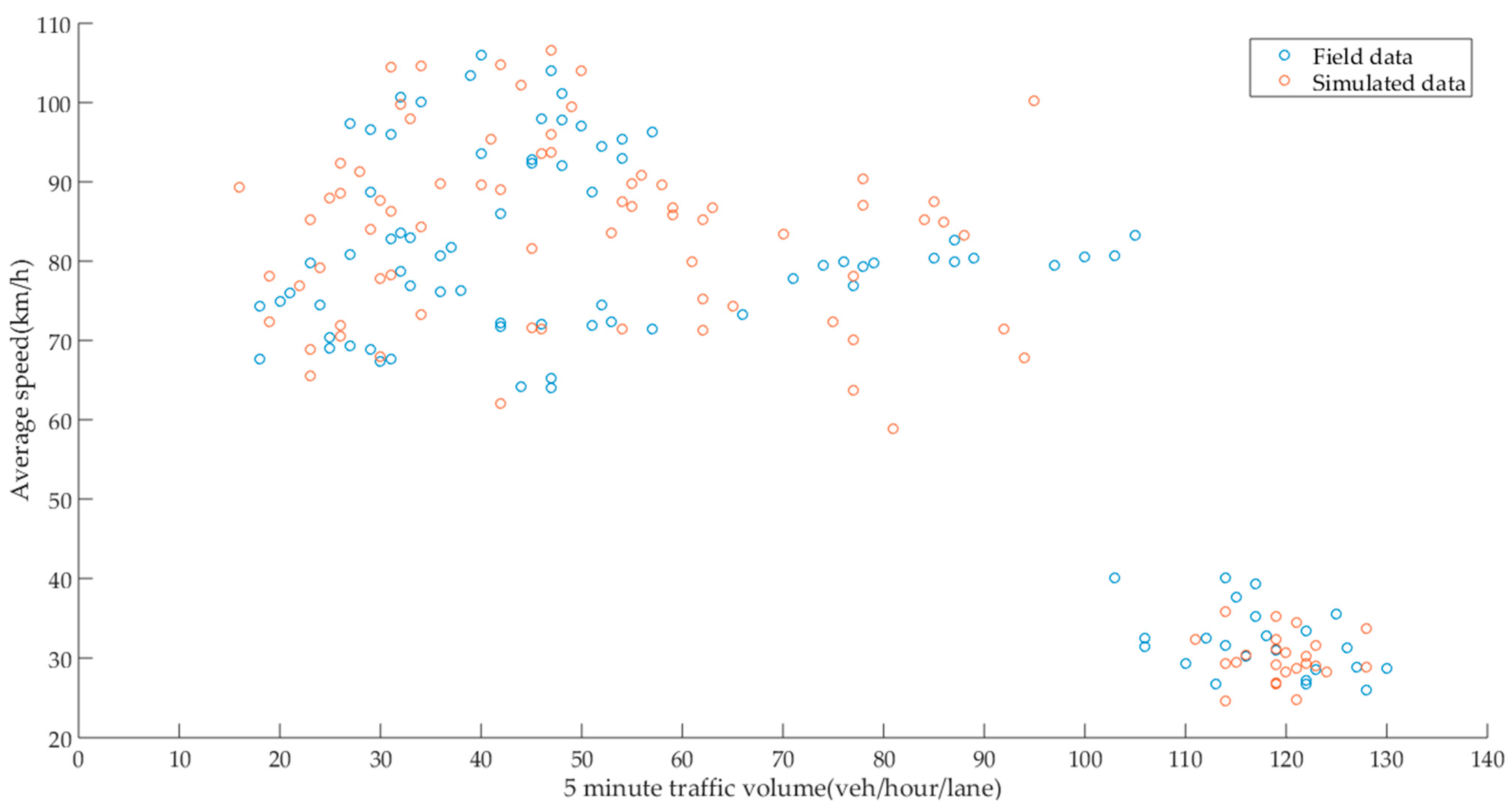
Figure 9 displays the speed-volume relationship of the field data and the simulated data generated by the cellular automata model. The blue dots represent the field data and the red dots represent the simulated data. Generally, the simulated data matches well with the field data. The Root Mean Squared Error (RMSE) between the field data and the simulated data for the traffic volume and the average speed are 6.9124, and 9.0095 respectively. The R² value of the traffic volume simulation and the average speed simulation are 0.9645, and 0.8944 respectively, which indicates the cellular automata model could simulate traffic conditions on the research highway effectively.

4.3. Application of the Cellular Automata Model

The cellular automata model is used to simulate the traffic states before and after the hard shoulder is used as an extra lane. We collected four variables including the traffic volume, average speed, variance of speed and travel time of emergency rescue vehicles during traffic accidents. We run the simulation model for 10 times to eliminate the random error. The traffic accident location is randomly selected in each run.

Table 5. Change rate of traffic states before and after the hard shoulder is opened (in percentage).

Low Density
Speed Limit	Traffic Volume	Average Speed	Variance of Speed	Travel time of emergency rescue vehicles during traffic accidents
60 km/h	0.10	−2.59	−9. 40	6.20
80 km/h	1.33	−1.70	−8.45	2.02
100 km/h	0.71	−0.84	−1.34	0.08
120 km/h	0.09	2.10	−7.78	5.07
Moderate density
Speed limit	Traffic volume	Average speed	Variance of speed	Travel time of emergency rescue vehicles during traffic accidents
60 km/h	1.57	−6.81	−11.39	−1.02
80 km/h	0.05	−0.73	−12.99	−3.10
100 km/h	−0.71	6.15	−13.95	0.08
120 km/h	0.25	10.19	−17.67	3.31
High density
Speed limit	Traffic volume	Average speed	Variance of speed	Travel time of emergency rescue vehicles during traffic accidents
60 km/h	23.06	5.58	2.96	34.07
80 km/h	24.09	10.07	9.74	74.93
100 km/h	24.65	19.43	17.38	125.67
120 km/h	24.46	12.49	13.25	154.77

describes the change rate of the variables before and after the hard shoulder is opened.

$$\mathrm{g}=\frac{y^{\prime }-y}{y}\ast 100$$

(9)

where, $y^{\prime }$ represents the variable obtained when the hard shoulder is closed, y refers to the variables obtained after the harder shoulder is opened during the simulation, g is the change rate in percentage.

As indicated in Table 5, when the density is low or moderate, the variations of the traffic states before and after the hard shoulder is used as running lane is not significant. When the density is high, opening the hard shoulder for running vehicles could improve the traffic volume by more than 20% under various speed limit, and the average speed could also be improved. However, opening the hard shoulder in the high-density condition also brings side effect of increased speed variance and travel time of emergency rescue vehicle.

4.4. Results of Decision Optimization Method

One key issue in this study is to determine the optimal traffic state and speed limit of opening hard shoulders. We use cellular automata model to simulate traffic states when the hard shoulder is opened for normal vehicle operation. Four variables including the traffic volume, the average speed, the speed variation and the travel time of emergency rescue vehicles to the accident location are collected to evaluate traffic conditions under different speed limits of the hard shoulder. We use the factor analysis method in combination of TOPSIS method to establish the evaluation standard. The factor analysis method is used to identify appropriate weights of the four variables and TOPSIS method is used to rank the different hard shoulder operation strategies. The hard shoulder had two states: opened and closed. When the state of hard shoulders changed, changes of the traffic volume and the average speed are used as benefit attributes, changes of the variance of speed and the travel time of emergency rescue vehicles during traffic accident are used as cost attributes.

KMO test and Bartlett sphere test are used to determine the correlation of data and whether it conforms to the requirement of factor analysis [34]. The value of KMO test is between 0 and 1. The higher the KMO value, the better effect of factor analysis. Generally, when the value of KMO test is greater than 0.5, it indicates that the factor analysis is suitable.

In this research, the value of KMO test is calculated as 0.78, which indicates the validity of using factor analysis. The weight of traffic volume, average speed, variance of speed and travel time of emergency rescue vehicles during traffic accident are computed as 0.26, 0.23, 0.25, 0.26 respectively. Four different speed limits including 60 km/h, 80 km/h, 100 km/h and 120 km/h are considered under three categories of traffic states including the high density, moderate density and low density. The TOPSIS method is used to rank the 12 alternatives.

Table 6. Results of the Optimization Method.

Cluster Label	Speed Limit of Hard Shoulder	${\mathit{f}}_{\mathit{i}}^{*}$	Rank of TOPSIS
1	60 km/h	0.1602	10
1	80 km/h	0.1815	9
1	100 km/h	0.2723	6
1	120 km/h	0.2348	8
2	60 km/h	0.1042	12
2	80 km/h	0.1417	11
2	100 km/h	0.2451	7
2	120 km/h	0.2923	5
0	60 km/h	0.5099	4
0	80 kn/h	0.6759	3
0	100 km/h	0.9122	1
0	120 km/h	0.8495	2

displays the results of the calculation.

As Table 6 shows, the rank is higher when the cluster label is 0, which indicates opening hard shoulder as an extra lane can achieve better effect when the traffic density is high. When the traffic is congested, opening the hard shoulder could provide an extra lane for the excessive traffic volume. However, when the traffic is not congested, an extra lane would not bring significant improvement of traffic condition. In addition, Table 6 indicates that the speed limit for the hard shoulder lane could be set as 100 km/h to achieve better effect. If the speed limit is too high, the speed variations would increase, which may lead to potential traffic incidents. If the speed limit is too low on the hard shoulder lane, the drivers may be discouraged to use the extra lane. In our case, 100 km/h is found to be optimal. The reason maybe attribute to the speed limit of the adjacent lane is also 100 km/h. For other highways, if the speed limit of the adjacent lanes is set differently and the number of the lanes of the highway are different, the optimal speed limit for the hard shoulder lane may be different. However, similar methodology could be applied to identify the optimal speed limit and the optimal traffic condition for other highways.

5. Discussion and Conclusions

This paper proposed an optimization method for identifying the proper traffic condition and speed limit for hard shoulder running strategy. Our work contributes to the traffic management strategies in the following aspects: (1) For different traffic condition, we could implement different traffic management strategy to maximize traffic control efficiency. We used clustering method to group similar traffic states and tested four clustering methods including the K-Means, agglomerative, mean shift and spectral clustering method. The silhouette score, DBI and Caliski-Harabaz Score are used to compare the clustering effect and the results showed that the K-Means method with three traffic state categories is best. (2) We used the cellular automata model to examine the traffic condition when the hard shoulder is opened. The parameters of the cellular automata model include the probabilities of random deceleration, slow start and lane change are calibrated using real-world traffic data. In addition, we simulated traffic accident condition to evaluate the influence of hard shoulder running strategy on the safety aspect. (3) We proposed that four variables including the traffic volume, average speed, variance of speed and travel time of emergency rescue vehicles during traffic accident should be used as indicators to compare various hard shoulder running strategies. The traffic volume and the average speed could reflect the traffic efficiency, meanwhile the variance of speed and the travel time of emergency rescue vehicles during traffic accident could indicate the level of safety. We used factor analysis method to determine the weights of the four variables, and TOPSIS is used as the decision-optimization method to identify the optimal traffic condition and speed limit to open the hard shoulder as an extra driving lane.

The methodology framework to calculate the optimal traffic condition and speed limit as proposed in this paper could be applied to other highways where the width of the hard shoulder satisfy the traffic operation requirement (>3.25 m). In our research, the result suggested that the hard shoulder could be opened when the traffic density is high and the speed limit should be set as 100 km/h to achieve best performance. However, when applied to other highway segments with different geometric design and different speed limits, the result may be different since the traffic conditions may be different. In order to ensure traffic safety when applying hard shoulder running strategy, dynamic message signs and traffic surveillance devices such as loop detectors, video cameras, and radar detectors should be equipped along the roadway. The dynamic message signs are prerequisites since the drivers need to be informed whether the hard shoulder is opened or closed in a certain segment. The traffic surveillance devices are needed to collect traffic states information. For practice, traffic engineers could predict traffic states based on historical traffic statistics and make reasonable decisions in advance on when to open the hard shoulder. The traffic surveillance devices are also needed in case of accidents, the hard shoulder should be closed immediately to help reduce the travel time of emergency rescue vehicles.

For future research, we could extend our current research in the following directions: (1) We could further evaluate the safety issues that may be aroused by applying the hard shoulder running strategy. More simulations should be conducted to study traffic conditions under accidents of various severity levels, which may block more than one lane and larger road surface. (2) We could consider dividing the highway into different segments by dynamic message signs and apply more flexible control strategies. The spacing of the dynamic message signs could be optimized, and the speed limits for each segment under various traffic condition could be controlled using dynamic optimization methods.

References

1. Wang, S.; Djahel, S.; Zhang, Z.; McManis, J. Next Road Rerouting: A Multiagent System for Mitigating Unexpected Urban Traffic Congestion. IEEE Trans. Intell. Transp. Syst. 2016, 17, 2888–2899. [Google Scholar] [CrossRef] [Green Version]
2. Schrank, D.; Eisele, B.; Lomax, T. TTI’s 2012 Urban Mobility Report Powered by INRIX Traffic Data; Texas A&M Transportation Institute Texas, A&M University System: College Station, TX, USA, 2011. [Google Scholar]
3. Jiang, P.; Liu, L.; Cui, L.; Li, H.; Shi, Y. Congestion prediction of urban traffic employing SRBDP. In Proceedings of the 2017 IEEE International Symposium on Parallel and Distributed Processing with Applications and 2017 IEEE International Conference on Ubiquitous Computing and Communications (ISPA/IUCC), Guangzhou, China, 12–15 December 2018; pp. 1099–1106. [Google Scholar]
4. Dutta, N.; Boateng, R.A.; Fontaine, M.D. Safety and Operational Effects of the Interstate 66 Active Traffic Management System. J. Transp. Eng. Part A Syst. 2019, 145, 4018089. [Google Scholar] [CrossRef]
5. Lemke, K. Hard Shoulder Running as a Short-Term Measure to Reduce Congestion. In Proceedings of the Interntional Symposium on Highway Geometric Design, Valencia, Spain, 1–5 June 2010. [Google Scholar]
6. Geistefeldt, J. Operational Experience with Temporary Hard Shoulder Running in Germany. Transp. Res. Rec. 2012, 2278, 67–73. [Google Scholar] [CrossRef]
7. Brilon, W.; Lippold, C. Country Report--Germany: A New Concept for Highway Design Guidelines in Germany. In Proceedings of the International Symposium on Highway Geometric Design, Chicago, IL, USA, 29 June–1 July 2005. [Google Scholar]
8. Guerrieri, M.; Mauro, R. Capacity and safety analysis of hard-shoulder running (HSR). A motorway case study. Transp. Res. Part A Policy Pract. 2016, 92, 162–183. [Google Scholar] [CrossRef]
9. Lemke, K.; Irzik, M. Temporary Use of Hard Shoulders—Experiences and Economic Assessment; Traffic Planning Highway Disaster Safety Analytical Section, Federal Highway Research Institute: Bergisch Gladbach, Germany, 2016. [Google Scholar]
10. Gitelman, V.; Hakkert, S.; Zilberstein, R.; Grof, T. Bus Operations on Hard Shoulders during Congested Morning Hours—A Pilot Evaluation in Israel. Transp. Res. Procedia 2016, 14, 1144–1153. [Google Scholar] [CrossRef] [Green Version]
11. Kellermann, G. Experience of Using the Hard Shoulder to Improve Traffic Flows. Traffic Eng. Control 2000, 41, 412–414. [Google Scholar]
12. Chase, P.; Avineri, E. Maximizing Motorway Capacity Through Hard Shoulder Running: UK Perspective. Open Transp. J. 2008, 2, 7–18. [Google Scholar] [CrossRef]
13. Farrag, S.G.; Outay, F.; Yasar, A.U.H.; El-Hansali, M.Y. Evaluating active traffc management (ATM) strategies under non-recurring congestion: Simulation-based with benefit cost analysis case study. Sustainability 2020, 12, 6027. [Google Scholar] [CrossRef]
14. Berger, W.J.; Maurer, P. Emergency bays versus emergency lanes on motorways-A cost benefit analysis. In Proceedings of the 10th International Conference-Traffic Safety on Two Continents, Malmo, Sweden, 20–22 September 1999; pp. 1–12. [Google Scholar]
15. Bergmeister, K.; Benesperi, C.; Cavestro, R.; Mauro, R. New Information technologies on the Brenner Freeway. In Proceedings of the 2nd Int. SIIV Congress on New Technologies and Modelling Tools for Roads: Applications to Design and Management (CD-ROM), Italian Society of Road Railway Airport, Ancona, Italy, 27–29 October 2004. [Google Scholar]
16. Zhou, W.; Yang, M.; Lee, M.; Zhang, L. Q-Learning-Based Coordinated Variable Speed Limit and Hard Shoulder Running Control Strategy to Reduce Travel Time at Freeway Corridor. Transp. Res. Rec. 2020, 2674, 915–925. [Google Scholar] [CrossRef]
17. Karan, A. An Integrated Variable Speed Limit with Dynamic Hard Shoulder Running for Urban Freeway Traffic Control. Schulich Sch. Eng. 2018. [Google Scholar] [CrossRef]
18. Chen, Z.; Jiang, Y.; Sun, D. Discrimination and Prediction of Traffic Congestion States of Urban Road Network Based on Spatio-Temporal Correlation. IEEE Access 2020, 8, 3330–3342. [Google Scholar] [CrossRef]
19. Shen, X.; Chen, J. Study on prediction of traffic congestion based on LVQ neural network. 2009 Int. Conf. Meas. Technol. Mechatronics Autom. ICMTMA 2009 2009, 3, 318–321. [Google Scholar] [CrossRef]
20. Jain, A.K. Data clustering: 50 years beyond K-means. Pattern Recognit. Lett. 2010, 31, 651–666. [Google Scholar] [CrossRef]
21. Yamasaki, R.; Tanaka, T. Properties of Mean Shift. IEEE Trans. Pattern Anal. Mach. Intell. 2020, 42, 2273–2286. [Google Scholar] [CrossRef]
22. Huang, D.; Wang, C.D.; Wu, J.S.; Lai, J.H.; Kwoh, C.K. Ultra-scalable spectral clustering and ensemble clustering. IEEE Trans. Knowl. Data Eng. 2020, 32, 1212–1226. [Google Scholar] [CrossRef] [Green Version]
23. Kakkavas, G.; Karyotis, V.; Papavassiliou, S. A Distance-based Agglomerative Clustering Algorithm for Multicast Network Tomography. In Proceedings of the ICC 2020–2020 IEEE International Conference on Communications (ICC), Dublin, Ireland, 7–11 June 2020; pp. 1–7. [Google Scholar] [CrossRef]
24. Hua, W.; Yue, Y.; Wei, Z.; Chen, J.; Wang, W. A cellular automata traffic flow model with spatial variation in the cell width. Physica A 2020, 556, 124777. [Google Scholar] [CrossRef]
25. Ad, V.; Networks, H.; Cheng, S.; Horng, G.; Chou, C. Using Cellular Automata to Form Car Society in Vehicular Ad Hoc Networks. IEEE Trans. Intell. Transp. Syst. 2011, 12, 1374–1384. [Google Scholar] [CrossRef]
26. Mamei, M.; Roli, A.; Zambonelli, F.; Università, I. Emergence and Control of Macro-Spatial Structures in Perturbed Cellular Automata, and Implications for Pervasive Computing Systems. IEEE Trans. Syst. Man, Cybern. Part A Syst. Hum. 2005, 35, 337–348. [Google Scholar] [CrossRef] [Green Version]
27. Hamurcu, M.; Eren, T. Strategic planning based on sustainability for urban transportation: An application to decision-making. Sustainability 2020, 12, 3589. [Google Scholar] [CrossRef]
28. Gong, Y. Business performance evaluation of sports industry listed-companies based on factor analysis. In Proceedings of the 2017 International Conference on Smart Grid and Electrical Automation (ICSGEA), Changsha, China, 27–28 May 2017; pp. 450–453. [Google Scholar] [CrossRef]
29. Han, D.; Ren, X. Financial risk assessment based on factor analysis model. J. Phys. Conf. Ser. 2020, 1616. [Google Scholar] [CrossRef]
30. Hwang, C.L.; Yoon, K.; Hwang, C.L.; Yoon, K. Multiple Attribute Decision Making. Lect. Notes Econ. Math. Syst. 1981, 404, 287–288. [Google Scholar]
31. Shih, H.; Shyur, H.; Lee, E.S. An extension of TOPSIS for group decision making. Math. Comput. Model. 2007, 45, 801–813. [Google Scholar] [CrossRef]
32. Zhang, J.; Wang, C.; Liu, L.; Guo, H.; Liu, G.; Li, Y.; Deng, S. Science of the Total Environment Investigation of carbon dioxide emission in China by primary component analysis. Sci. Total Environ. 2014, 472, 239–247. [Google Scholar] [CrossRef] [PubMed]
33. Wang, T.C.; Chang, T.H. Application of TOPSIS in evaluating initial training aircraft under a fuzzy environment. Expert Syst. Appl. 2007, 33, 870–880. [Google Scholar] [CrossRef]
34. Chen, S.; Fan, Y.; Cao, Y.; Khattak, A. Assessing the relative importance of factors influencing travel happiness. Travel Behav. Soc. 2019, 16, 185–191. [Google Scholar] [CrossRef]
Figure 1. Traffic Volume of the Highway Segment.
Sustainability 13 01822 g001
Figure 2. Average Speed of the Highway Segment.
Sustainability 13 01822 g002
Figure 3. Boxplot of traffic volume on each lane.
Sustainability 13 01822 g003
Figure 4. Boxplot of the average speed on each lane.
Sustainability 13 01822 g004
Figure 5. Flow chart of the methodology.
Sustainability 13 01822 g005
Figure 6. Bar chart of Silhouette score.
Sustainability 13 01822 g006
Figure 7. The silhouette score plot of K-Means.
Sustainability 13 01822 g007
Figure 8. Scatter plot of three traffic states.
Sustainability 13 01822 g008
Figure 9. Comparison of the field data and the simulated data.
Sustainability 13 01822 g009