Abstract
The Indonesian government needs to maintain around 231,000 school buildings in active use. Such a portfolio of buildings given the diversity of locations, limited maintenance budget, and deterioration rates varied by different building conditions presents many challenges to effective maintenance planning. Many of those schools had been reported to be aging and in a degenerated condition. However, contemporary practice for the planning method of Indonesia’s building maintenance program applies reactive maintenance strategies with a single linear deterioration rate. Such methodology cannot properly guarantee the sustainability of those school buildings. Therefore, this study attempts to examine a different approach to Indonesia’s building maintenance planning by adopting a preventive maintenance strategy using the deterioration rate model proved by historical data from a previous study. This study develops an optimization model with varied deterioration rates and considers the budget limitation, by utilizing a Constraint Programming (CP) approach. The proposed model achieves the minimum maintenance cost for a real case of 41 school buildings under different deterioration rates to ensure adequate building conditions and maintain expected levels of service. Finally, research analysis also proves that this new preventive maintenance model has potential to deliver superior capability for assisting building maintenance decisions in Indonesia’s government.
1. Introduction
Building maintenance is widely acknowledged as a critical issue throughout the building management life cycle to prevent building deterioration [1,2] and to ensure building safety and comfort [3]. Several challenging issues for building maintenance topics, such as maintenance budget [4], demand for safety and serviceability from the organization or user [5], and difficulties in assessing and predicting the future of the facility condition [6], have been receiving great attention in recent years. Especially from the maintenance budget perspective, over a building’s life cycle, operation and maintenance costs can account for 50–80% of the total cost [4].
This study adopts school buildings as a case study to discuss different aspects of building maintenance problems since school buildings are high-priority public facilities to preserve from the public asset management point of view. Given the importance of educational facility preservation, some nations have emphasized the renovation of existing school buildings and launched school building modernization programs to ensure building sustainability [7,8,9,10]. Meanwhile, the maintenance of school buildings in Indonesia remains a scattershot affair [11]. Comparing with those developed countries with an advanced building maintenance program, this study is then inspired to conduct in order to accelerate a systematic approach for the issues of school building maintenance in Indonesia.
Today in Indonesia, the number of buildings is up to 170,000 elementary schools, 35,000 junior high schools, 20,000 general senior secondary schools, and 6000 vocational senior secondary schools [12]. The Ministry of National Education and Culture recently reported that 182,500 classrooms are severely compromised [13]. Utami [14] reported extensive damage in classrooms in Central Java Province. School buildings actually collapsed in West Jakarta in 2017 [15] and in Pasuruan East Java in 2019 [16]. All accidents happened due to the aging of building structures. These events have occurred without precaution and were caused by the neglect of proper building maintenance. Therefore, proper maintenance should be performed in different ways that depend on building agency policy, building environment, building function, and building existing condition. Moreover, delays in maintenance or repair will worsen building deterioration and make maintenance costs higher [17]. Such conditions create a challenge for the building agency to perform effective maintenance.
To aid problem-solving, this study aims to develop an optimization model of building maintenance schedules for a finite time horizon that considers the building deterioration rates. The main objectives of the proposed model are listed as follows: (1) an optimal decision to select a proper building maintenance plan to execute maintenance action at a certain time based on the building condition and the available annual maintenance budget; (2) a solution of preventive maintenance strategy that satisfies the building target service time and ensure the building condition in an acceptable condition. This paper adopts the Constraint Programming (CP) technique to develop the optimization model with varied deterioration rates to solve building maintenance problems under annual budget limitations. The proposed model is then validated using the case of school buildings in Tangerang city near Jakarta.
The following sections of this paper are organized as follows: In Section 2, the building maintenance problem is defined from previous research works, and the conceptual idea of building maintenance problems regarding research flow and data preparation is discussed. The methodology of the proposed preventive maintenance model is introduced, and model formulation is presented in Section 3. In Section 4, the results of the optimization model for a case of 41 school buildings are discussed and analyzed. Lastly, Section 5 concludes the research findings and provides a suggestion for future research.
2. Prior Studies
Maintenance is a combined technical and administration activity, including supervision to restore a particular element to a condition in which it adequately fulfills performance requirements [18]. According to Au-Yong et al. [19], maintenance management is the process that performs maintenance services to satisfy the organizational necessity. Moreover, cost-effective maintenance strategies include the performance of maintenance measures and implementation of the preventive and corrective measures at the proper time [20].
This study’s maintenance strategy refers to preventive maintenance. For building managers, building deterioration is a principal and ongoing concern throughout building service life [21]. Previous studies suggested that preventive maintenance strategy by defining particular deterioration models and setting priority criteria is an alternative solution to solve those hindrances [5,18,22,23]. The preventive maintenance strategy entails a regular maintenance schedule to ensure adequate building service and functionality throughout its lifecycle [24].
Building reliable maintenance can be started by establishing a deterioration model to govern decision-making in maintenance management [6,23,25]. Building maintenance actions are complicated by different deterioration rates among various building’s functions and locations, as well as coastal conditions, which contribute to more rapid deterioration [23]. Building location also influences other factors that determine deterioration of building facades including concrete formulation, color, texture surface, and finishing surface type [26].
This has prompted work in infrastructure maintenance management to develop optimization strategies that maximize maintenance performance while minimizing costs for roads [27,28,29,30] and bridges [31,32,33,34]. Particularly in the domain of building maintenance management, some researchers have sought to develop decision-making models to optimize building performance under limited budget conditions [22,24,35,36]. Overall, this study deals with a preventive maintenance strategy with various deterioration rates of building conditions. We formulate this problem using the Constraint Programming (CP) technique to develop the optimization model consider the budget limitations to perform the preventive maintenance. The model is then validated on school buildings in Tangerang city near Jakarta. CP is an operations research technique as a computational method and has been advantageously used to solve many optimization problems due to its effectiveness in resolving combinatorial search problems by representing the relations among decision variables as constraints and assigning the objective function [37,38]. As an algorithm for solving optimization problems in project scheduling, CP has been shown to be an applicable and efficient technique that is adopted by Liu [39], Tang and et al. [40], Menesi and Hegazy [41], as well as Zou and Zhang [42].
3. Methodology
3.1. Research Process of Building Maintenance Problem
The research methodology of the proposed model is divided into two stages: (1) data preparation stage, (2) optimization model development stage. The experimental process of this study begins with the data collection of the selected school buildings. As a hard constraint of building maintenance problem, the assessment on annual budget approval from the responsible public sector must be also taken into consideration for the data preparation stage. The detailed definition of other necessary data for a good preventive management strategy, such as building condition index (BCI) value for each building and classification rules of deterioration rates, will be presented in the following subsections. Figure 1 illustrates the research flow of the proposed model for the building maintenance problem.
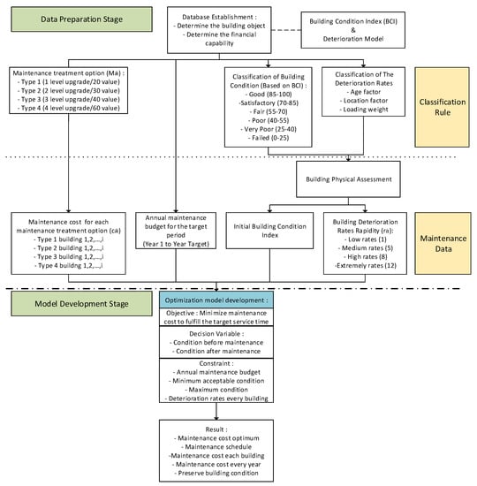
Figure 1.
Research flow chart of building maintenance problem.
The factors that make life cycle forecasting so difficult are future operating costs, maintenance costs, and discount rates [43,44]. Since it is difficult to forecast the lifecycle cost (LCC) of the facility precisely, then LCC is normally assumed as a constant value especially for the purpose of maintenance planning [45]. Therefore, the discount rate is not considered in this research. The LCC analysis is based on time- and cost-related variables and the lifecycle span for a facility is required to evaluate for facility service life. Thus, the building service time in the proposed model is assumed to be the building lifecycle to estimate maintenance frequency and cost [24]. In reality, the demand for annual maintenance costs always exceeds the annual maintenance budget. Therefore, the consideration of the annual maintenance budget is then a crucial constraint to influence maintenance actions.
3.2. Building Maintenance Data Preparation
3.2.1. Building Condition Index (BCI) and Classification of Building Condition
A Building Condition Index (BCI) assessment is used to measure and represent the physical condition of a building component. The BCI obtained from the condition inspection undertaken using a standardized condition assessment process. The calculation basis of the BCI equation used in this study is adopted from Grussing and Liu’s [35] research. The BCI was adopted from road pavement assessments, with the condition index expanded for building roofs and generalized building components [35]. Table 1 presents the BCI scale from 0 to 100, with 100 as the best building condition.

Table 1.
Value and condition description of building condition index (BCI).
Based on the condition described in Table 1 to ensure building safety and serviceability, this study aims to maintain the minimum condition in the proposed model of at least 40 according to Grussing and Liu’s work [35] to ensure sustainable building performance. BCI value will be used to define the initial building condition and an important parameter for evaluating the overall building condition in the proposed model.
3.2.2. Deterioration Model and Classification of Deterioration Rates
Most building maintenance strategies use a deterioration model to predict the building’s future condition, creating a condition index to assess and measure building conditions. This deterioration model presumes that the future condition index is a function of time after the latest maintenance treatment. This study applies two different types of deterioration rates. The first type is a 2% depreciation rate based on specifications from the Indonesian Ministry of Public Works and Housing [46], shown in Equation (1). The second type is the BCI assessment equation developed by Grussing in 2006 and 2014 [35,47]. The three-parameter Weibull distribution of the Grussing deterioration model adopted in this study was also utilized by Strzelecki [48] to determine the fatigue limit of the round drew steel bar. Some scenario conditions are stipulated in the maintenance management cycle to validate the proposed model.
Considering several diversified factors like the building age, building location, and building loading weight based on the building physical assessment, four types of rapidity deterioration rates are then determined. Wu and Lepech [49] mentioned that chloride-induced corrosion impacts the deterioration behavior of reinforced concrete structures. Prieto et al. [50] stated that different building locations result in different deterioration rates because of climate factors. Furthermore, Faqih and Zayed [51] declared that building environment and occupation utilization both are the influence factors of building deterioration. The building with the oldest age and hazardous locations, as well as most frequent use, will have the fastest deterioration rates. On the contrary, the building with the youngest age and a relatively safe environment, as well as minimum use will have the slowest deterioration rates. The value range to differentiate rapidity deterioration is shown in Table 2, where different values are set by the process of enormous trial and error best-fits of the deterioration curve after we acquired building condition data. Those values will be applied to the deterioration behavior of Equations (4) and (5). Based on these four types of rapidity deterioration value, this study then classifies all selected buildings into four groups with different deterioration rates.
Table 2.
Value and classification of building rapidity deterioration rate.
3.2.3. Maintenance Strategy
The idea of preventive building maintenance strategy attempts to preserve the building condition for all selected buildings above the minimum service level under a tight maintenance budget, where the minimum BCI value of an acceptable condition is 40. Four specific maintenance treatment options to upgrade the building condition are adopted. Each maintenance treatment option has a different ability to upgrade building conditions with different improvements to the BCI value and its corresponding maintenance cost. The maintenance option with the greatest BCI improvement corresponds to the most expensive maintenance cost, and vice versa. This concept is shown in Figure 1 and has a similar maintenance scheme for upgrading building structure conditions as proposed by Shuie et al. [52]. Moreover, the estimation of maintenance costs in this study is conducted by identifying building features, also through the historical maintenance data of public sectors. The maintenance costs are dependent on the building scale and features of the RC building structure.
3.3. Constraint Programming
It can be difficult to determine the best maintenance treatment option under a limited budget and a variety of deterioration conditions for several buildings. To address this difficulty, this study adopts constraint programming (CP) in developing the optimization model. CP has been widely used in previous studies to solve linear project scheduling problems for construction crews [39], schedule optimization given limited resources [53], multimode resource-constrained project scheduling [41], and dual-level multi-project scheduling for optimal resource allocation decisions among multiple concurrent prefabrication projects [54].
Constraint programming prevails the benefits of constraint propagation and systematical solution-seeking methods to effectively identify an optimal solution [54]. Constraint propagation, known as the consistency technique, eliminates values from variable domains that are not included in any solution or will generate infeasible solutions; thus reducing the search space and enhancing search efficiency [42,55]. There is a three-stage process of CP in dealing with optimization problems, that is, problem specification, consistency techniques, and systematic solution-seeking strategies to perform problem-solving [37,56]. Problem specification in CP optimization is defined by utilizing the subsequent structures: (1) a set of variables X = {x1, x2,… xn} in the proposed model to denote the building, maintenance treatment option, year, and priority value; (2) there exists a finite set domain of feasible values for every variable xi, such as building number, year, and cost for each maintenance treatment; and (3) a set of constraints f restricting possible concurrent and recognizable variable values. The constraints in this study include acceptable building conditions, building priority status, and maintenance budget.
The consistency techniques approach is applied to improve the search efficiency for acquiring solutions by removing inconsistent values from the variables domain [56,57]. CP provides three primary consistency techniques including node consistency, arc consistency, and path consistency [57]. The node consistency technique is the most straightforward technique to deal with unary constraints; the values from variable domains with unary constraints on the appurtenant variable are removed by using this technique [37,56]. The most general technique used is the arc consistency technique, the values from the variable domain with binary constraint is removed by using this technique. Lastly, path consistency removes relevant inconsistent values by employing three or more variables [37,56].
The propagation mechanism is implemented by the CP solution searching algorithm, by acquiring the objective function as a constraint while solving an optimization problem. The upper or lower bounds of the constraint are substituted after identifying a better objective function value. The solution searching process starts from the main objective, overall maintenance cost minimization, and related variables. The propagation constraints for reducing variable domains are obtained by using the consistency checking technique. Then, the variables and objects are stipulated as components of an empty set and treated as an initial solution. The BT searching strategy is used in this optimization algorithm to select relevant decision variables to promote search efficiency, then the key variables are searched in order with the following rules: (1) binary variable (Sijk) and (2) variable of maintenance treatment option (Mik), and the smallest value in each variable domain will become the starting point of the solution-searching process. Formerly the solution is an empty set, then, after acquiring a better value, this solution is substituted for the former solution. The current solution will be kept for a while when the present moves identify a worse solution up till when the next move engages in the case required. During each move, the solution information will be updated, and new constraints are then provided for constraint propagation and variable domain reduction. Furthermore, the solution re-searching and updating process is repeated for empty every variable domain. This process will quickly bind the optimal values from the variables’ domains, and the suggested optimization algorithm can acquire the optimal solution. [39]. The optimization algorithm is illustrated in Figure 2, thus an optimal solution for the objective can be assured.
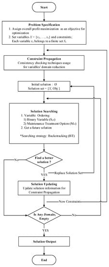
Figure 2.
CP optimization procedure for building maintenance problems.
3.4. Model Formulation
This study focuses on developing the CP formulation model using the IBM ILOG CPLEX CP Optimizer as a solver engine and using ILOG OPL language for model setup and problem description [58]. The proposed model could be used in optimizing the maintenance strategies of a variety of buildings by minimizing the total maintenance cost within a given service life target.
This model consists of three parts, namely decision variables, constraints, and objective function. Each of these parts will be equipped with notations to describe the variable involved in the model. Table 3 presents the notation symbols.
Table 3.
Notations index, parameters, and variables.
In this CP model, there are three decision variables. The first decision variable is Sijk as the binary variable to determine the specific choice of maintenance strategy. The second decision variable, BCIij, represents the condition before maintenance in year one. The third decision variable is CAij, which indicates the condition after maintenance in the current year. Since the deterioration rate is a graphical line of the building condition index value over the years, the model is described with these specific constraints:
where the constraint in Equation (1) is determined by the condition before maintenance as the initial value of the condition index in year one for existing building conditions (bi1). Information for existing building conditions (bi1) is collected through building physical assessment. To accommodate the four different types of rapidity deterioration rates (ris) in the model formulation, this study applies Equations (2) and (3) respectively. Constraint Equation (2) is used to represent the deterioration rate based on the Indonesian Ministry of Public Works and Housing, and Equation (3) is used to represent the deterioration rate based on the modified Weibull probability model. The values of rapidity deterioration rates (ris) in Equations (2) and (3) are substituted from Table 2 to generate four types of different deterioration rates. The value of the decay parameter (di) is obtained by the trial and error process of historical data collection, this value is determined 2.1. Since the collected data does not show service life assessment, the adjustment service time (Tij) value in this study is assumed to be 1, with no adjustment needed. The terminal condition index (n) is the approximation of building condition at the end of service life that depends on the design plan of each building.
Equation (4) represents that the maintenance action is followed by the situation of existing Sijk, where mik improves the current condition of the select building, new BCIi,j becomes CAi,j+1. These two equations establish the deterioration graph for conditions before and after maintenance.
Based on Equations (4)–(6), the binary variable Sijk will be engaged when the building condition degrades almost under 40 BCI value, based on the rapidity deterioration rate of this building. Sijk will decide whether or not to perform maintenance, and which type of maintenance treatment to use. Equation (5) indicates that if a particular building is selected to be maintained according to a certain maintenance treatment option, the corresponding maintenance cost for the maintenance type maintenance option to upgrade the building condition is also determined. Equation (6) represents that if there is no maintenance treatment applied, the maintenance cost will not occur. Subsequently, the upgrading value from the chosen maintenance treatment is added to the index value condition before maintenance to obtain the index value condition after maintenance.
According to the index range shown in Table 1, Equations (7) and (8) create a range of acceptable building conditions. Equation (9) indicates that all buildings must be above 0 BCI value. The limited maintenance budget condition is described in the constraint Equation (10), where fj represents the total available maintenance budget every year, and cik represents the maintenance cost. The details for maintenance cost (cik) for each building and annual maintenance budget (fj) are provided in Table A1 in the Appendix A. The maintenance cost is chosen by binary variable Sijk, where maintenance cost (cik) offers four options to be selected for all maintenance actions of all buildings, subject to annual budget limitations (fj).
Constraint Equation (11) is formulated to keep the selected building in good condition in a certain year.
The model also can be set to preserve several buildings in good condition in the whole target service time by applying Equation (12).
The objective function of the proposed model is to assure sustainable building performance while minimizing total maintenance costs for a certain building setup during a specific service period, based on maintenance treatment options. This study performs the objective function as follows:
i = 1,2,….,l ; j = 1,2,…,y ; k = 1,2,….,n
This objective function will choose the most efficient maintenance treatment option subject to the available maintenance budget and recommend the most efficient maintenance plan for all selected buildings each year.
4. Case Study and Discussion
The case study in this study includes 41 school buildings in Tangerang from Kusnadi’s work [59]. The service target time is set for 15 years with varied annual budgets for each year, shown in Appendix A Figure A1. Annual budget limitations are assumed according to the financial ability of the Tangerang city government. Based on the physical assessment conducted by Kusnadi [59] and the local government, the 41 buildings have various initial conditions and are divided into four groups, based on different deterioration speed, as follows: (1) Building numbers 1–10 are grouped as group 1 with the slowest deterioration, (2) Building numbers 11–20 are grouped as group 2 with the medium deterioration, (3) Building numbers 21–30 are grouped as group 3 with the fast deterioration, (3) Building numbers 31–41 are grouped as group 4 with the fastest deterioration. The optimized results are used to evaluate the effectiveness of the two deterioration models.
4.1. Deterioration Model Scenario 1
The deterioration rate in this scenario is based on a linear rate. The simulation of maintenance decision planning conforms with the model’s assumptions. Figure 3a–d compare the before and after maintenance conditions for the 10 sample buildings, selected according to the deterioration rates group for good priority condition, and specific conditions for building 7 in Figure 3a, as well as building 29 in Figure 3c.
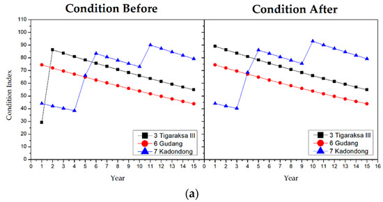
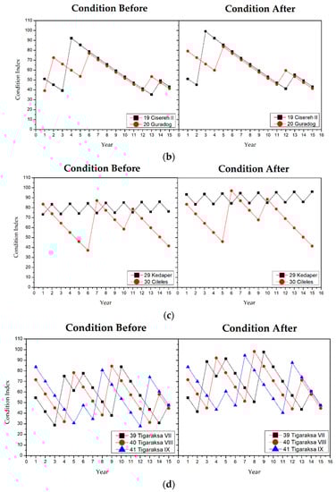
Figure 3.
(a) Condition before and after maintenance scenario 1 for the buildings in group 1. (b) Condition before and after maintenance scenario 1 for the buildings in group 2. (c) Condition before and after maintenance scenario 1 for the buildings in group 3. (d) Condition before and after maintenance scenario 1 for the buildings in group 4.
Most sample buildings before maintenance have condition index values below the minimum threshold value, except for building number 29 (Figure 3c) that is required to be consistently kept in good condition. Over the course of the 15-year maintenance period, all buildings must be maintained above the minimum acceptable condition. Comparing conditions before and after maintenance, we find that all buildings have a new condition index post-maintenance. Moreover, this condition confirms that the deterioration rate after maintenance equals the deterioration rate at the corresponding new condition state [60].
For building numbers 39, 40, and 41 in Figure 3d, due to the fast deterioration rates, the maintenance option chosen by the model is mainly maintenance option 4 to secure building service performance and the building safety condition. Hence, Figure 3d shows that all building conditions after maintenance preserve the building in the lowest satisfactory condition or above a 70 BCI value.
Based on Figure 3a–d, Table 4 presents the typical maintenance planning and the maintenance treatment options. Table 4 confirms that buildings with a slow deterioration rate need less maintenance than those with faster deterioration rates. Consequently, the building group with a faster average deterioration rate will require greater maintenance treatment, reflecting the findings of Farahani et al. [61] for the maintenance and renovation of multifamily buildings. Furthermore, buildings with the lowest condition index value will receive maintenance before other buildings in year one, except for building number 29 which is prioritized to be continuously maintained in good condition. From the results in Table 4, the maintenance cost information is established in Table 5. The total maintenance cost for 41 buildings during the 15-year service target is IDR 44,296,680,750.
Table 4.
Maintenance plan for all buildings in scenario 1.
Table 5.
Optimized maintenance cost for the 10 chosen sample buildings scenario 1.
4.2. Deterioration Model Scenario 2
This model has been widely used in previous studies and has been shown to be reliable for describing building deterioration rates [35,61,62]. The simulation performed in maintenance decision planning scenario 2 is still in line with the assumption in the proposed model. To represent the four different group deterioration rates and building priorities, 10 buildings are chosen to represent the before and after maintenance conditions in Figure 4a–d.
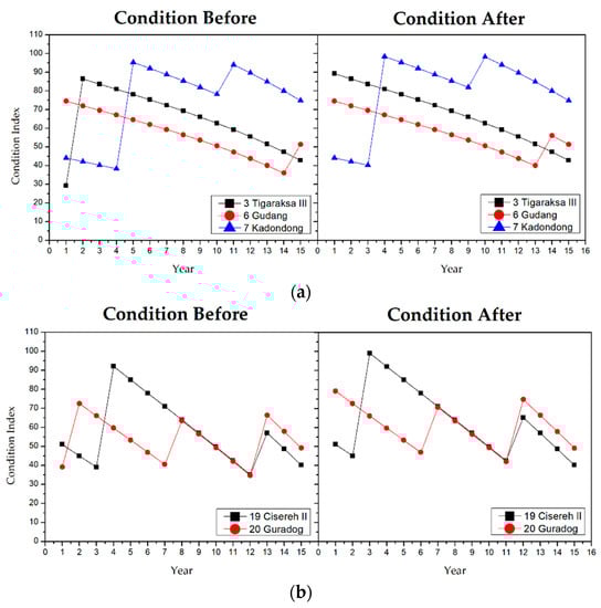
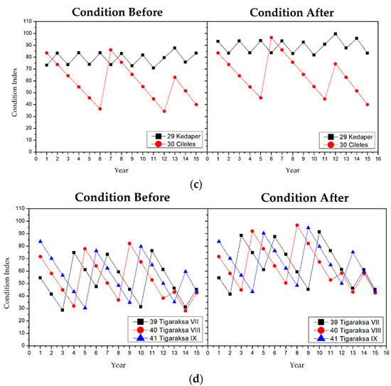
Figure 4.
(a) Condition before and after maintenance scenario 2 for the buildings in group 1. (b) Condition before and after maintenance scenario 2 for the buildings in group 2. (c) Condition before and after maintenance scenario 2 for the buildings in group 3. (d) Condition before and after maintenance scenario 2 for the buildings in group 3.
The non-linear model in scenario 2 features faster deterioration than the linear model in scenario 1, reflected by the higher number of buildings requiring maintenance in scenario 2.
In order to ensure building service performance, the maintenance option applied for building numbers 39, 40, and 41 with the fastest deterioration rates for scenario 2 in Figure 4d is mainly maintenance option 4, with the ability to upgrade the building condition with 60 value of BCI. Thus, the condition value of most buildings after maintenance is above 70 BCI value.
According to Figure 4a–d, the maintenance plan for scenario 2 can be decided, as shown in Table 6. The information in Table 6 emphasizes that buildings in scenario 2 with faster deterioration will require additional maintenance treatment, such as buildings 39 and 40, with the buildings with the fastest deterioration requiring four times as much maintenance as buildings 3 and 6. To ensure building sustainability, most of the maintenance treatments applied to the buildings in group 4 are maintenance treatment option 4, which has the highest upgradable capability and is also the most expensive. The chosen maintenance treatment confirms the upgrading ability, similar to the level of renovation proposed by Shiue et al. [52].
Table 6.
Maintenance planning for the 10 chosen sample buildings in scenario 2.
Comparing the results of Table 4 (for scenario 1) with those of Table 6 (for scenario 2), shows that scenario 2 requires more maintenance treatment. The divergence in maintenance treatments between scenarios 1 and 2 is only 1 (scenario 1 needs 29 maintenance and scenario 2 needs 30 maintenance), thus the difference in total maintenance between these two scenarios is not significant. The incidence of maintenance treatment option 4 increases from 9 in scenario 1 to 10 in scenario 2, while that for maintenance treatment option 3 increases from 1 in scenario 1 to 5 in scenario 2. Therefore, the maintenance cost in scenario 2 is higher than in scenario 1, as shown in Table 7. The same steps to create an annual maintenance budget are taken from maintenance planning, and identification of maintenance treatment options should be applied for each building for a given year. Total maintenance cost in scenario 2 is IDR 49,188,282,100.
Table 7.
Optimized maintenance cost for the 10 chosen sample buildings scenario 2.
Comparing the results for scenario 2 in Table 7 and scenario 1 in Table 5, we can notice increasing maintenance costs in scenario 2 for 8 out of all 10 buildings, with the exception of buildings 3 and 29 for which the maintenance cost remains consistent with scenario 1. Building 3 has the slowest deterioration rate and thus does not change significantly between the two scenarios. Building 29 is prioritized to be consistently maintained in good condition, thus maintenance treatment is identical for both scenarios. Building 20 incurs the highest percentage increase in maintenance costs (19.05%) while building 41 has the highest absolute increase due to its large size (IDR 335,964,000), though this only represents an increase of 6.06%.
The characteristic deterioration model in scenario 1 shows a slow deterioration rate, while that in scenario 2 is faster, leading to different amounts of maintenance treatment over the 15-year service period. With the number difference of maintenance treatment reflected in Table 8, in scenario 1, the 41 buildings require 96 maintenance treatments, as opposed to 107 in scenario 2. Regarding maintenance treatment option, the treatment number of maintenance option 4 (i.e., the most expensive treatment) is respectively 33 and 41 in scenarios 1 and 2.
Table 8.
Summary of maintenance treatment option.
4.3. Buildings with High Maintenance Priority
In terms of high maintenance priority, the existing buildings with severe damage conditions (below a value of 40 BCI) and having fast deterioration rates should be devoted more attention. This classification is common sense for facility management problems that have a budget limitation. Subsequently, this classification is used to evaluate the behavior of the model result in selected priority buildings and expected to help the building operator to define a particular building as having maintenance action priority.
Corresponding to this classification, Figure 5 and Figure 6 then confirm the result of the selected buildings by the proposed model for scenario 1 and scenario 2 respectively, where those selected buildings had shown the same characteristics as a Priority Building. These figures show 16 priority buildings in scenario 1 and 17 priority buildings in scenario 2. Further observation from these figures reveals that a building with a severe condition in the first year or one with a severe condition in the early years of service life will be promoted as a priority building. Those buildings are building numbers 3, 14, 31, 36, 37, and 40 for scenario 1, as well as building numbers 3, 20, 32, 33, and 37 for scenario 2. Moreover, most buildings have the characteristic of the fastest deterioration, such as building numbers 31, 36, 37, 38, and 40 for scenario 1, as well as building numbers 32, 33, 35, 37, 38, and 41 for scenario 2. Comparing buildings with the slowest deterioration rate, there is only one building in scenario 1 (building number 3) and two buildings in scenario 2 (building number 2 and 3). For example, building number 3 is selected as a priority building since this building has severe conditions in the first year. Based on those buildings’ characteristics shown in Figure 5 and Figure 6, maintenance option 4 (T4) is applied to most of those buildings.
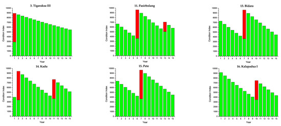
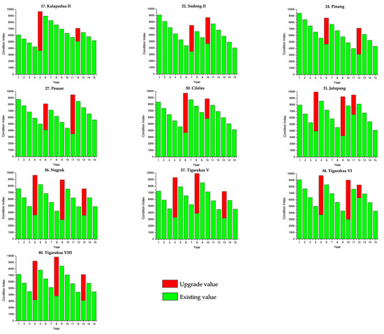
Figure 5.
Decision upgrading condition value of the selected priority building (Scenario 1).
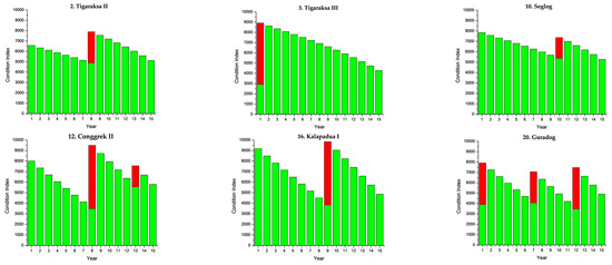
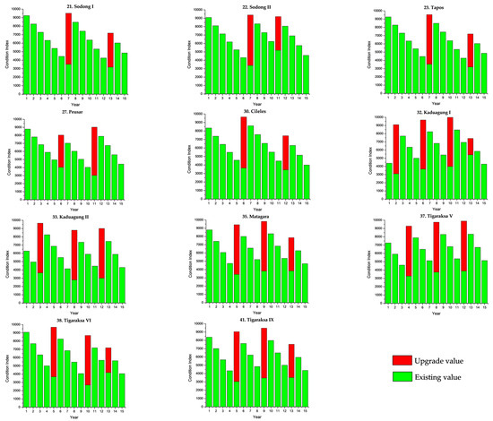
Figure 6.
Decision upgrading condition value of the selected priority building (Scenario 2).
According to the optimized result of the building conditions after maintenance, priority buildings have a better average condition than non-priority buildings. These facts are resumed in Table 9 for scenario 1 and Table 10 for scenario 2. From these Tables, it shows that the smallest average BCI values of priority building groups are 63.05 and 60.51 for scenario 1 and scenario 2, respectively. Comparing non-priority building groups, the smallest values are 53.56 and 57.88 for scenario 1 and scenario 2, respectively. Further results also disclosed that none of the buildings in priority building groups have an average condition scale value below 60.
Table 9.
Average building condition between priority and non-priority (Scenario-1).
Table 10.
Average building condition between priority and non-priority (Scenario-2).
The priority buildings with an average BCI value above 70 include those buildings with faster deterioration rates that usually result in a higher risk to be unserviceable. These buildings are building numbers 3 and 31 in scenario 1, as well as buildings number 16, 22, 32, 35, and 37 for scenario 2. Building number 3 in scenario 1 is an exception due to severe initial condition and slow deterioration rate. This result reflects a common-sense decision where the buildings with greater damage risk are treated as high priority for proper maintenance actions. Non-priority buildings with a BCI value average above 70 are not reflected in the same condition as a priority building, due to good initial conditions and slow deterioration rates.
5. Conclusions
In this paper, a novel CP-based optimization model for building maintenance problems is developed, and a case study of 41 existing school buildings with various sizes and conditions in Indonesia is analyzed. The analysis results with two types of deterioration rates applied to the proposed model are compared in the context of examining and improving building maintenance planning in Indonesia. The objective of the proposed model is to minimize overall maintenance costs over 15 years of service life for all selected buildings. Moreover, the proposed model is designed to be flexible and adaptable to the existing building condition, varied deterioration rates, annual budget limitation, as well as priority building preservation. The optimized result shows that the proper maintenance actions for the buildings with fast deterioration rates provide better average condition results for those buildings, and also none of those buildings have an average BCI value under 60.
Furthermore, the maintenance cost and the maintenance action frequency through scenario 2 are consistent with the demand for building upgrades in a comparable real-world situation. This result reveals that the imprecise factors of the linear deterioration rate adopted by the Indonesian government could be improved, and the proposed model is proved to illustrate building condition degradation in a more realistic and accurate way than the current practices of the Indonesian government agencies.
Overall, the optimization result, particularly in scenario 2, indicates the correct timing to execute specific maintenance actions for upgrading building conditions and avoiding a decline in building conditions under different annual budgets. This result reflects the capability of such an optimization model focused on sustainable building maintenance problems to ensure the optimal allocation of constrained financial resources. Moreover, this proposed model is suitable for a range of building maintenance problems faced by the building industry, especially for buildings operated by government agencies that receive annual budgets to maintain buildings within their areas of responsibility.
Future research and development of the proposed optimization model need to consider the changes in building energy efficiency performance concurrently with the degradation of building conditions. The aging of an existing building affects the building’s energy efficiency performance and leads to greater electrical power consumption. Future expansion of model development should consider energy cost in addition to maintenance cost to improve overall building energy performance.
Author Contributions
Conceptualization, S.-S.L. and M.F.A.A.; formal analysis, S.-S.L. and M.F.A.A.; investigation, S.-S.L. and M.F.A.A.; writing—original draft preparation, M.F.A.A.; writing—review and editing, S.-S.L. and M.F.A.A.; visualization, M.F.A.A.; supervision, S.-S.L. All authors have read and agreed to the published version of the manuscript.
Funding
This research received no external funding.
Institutional Review Board Statement
Not applicable.
Informed Consent Statement
Not applicable.
Data Availability Statement
Data generated or analyzed during the study are available from the corresponding author by request.
Conflicts of Interest
The authors declare no conflict of interest.
Appendix A. Supporting Tables and Figures of Buildings Data for the Case Study
Table A1.
Initial building condition index (bi1) and List of building maintenance cost based on maintenance treatment option (cik).
Table A1.
Initial building condition index (bi1) and List of building maintenance cost based on maintenance treatment option (cik).
| No | Building Name | Building Condition Index | Type 1 | Type 2 | Type 3 | Type 4 |
|---|---|---|---|---|---|---|
| 1 | Tigaraksa I | 86.43 | 172,608,000 | 241,651,200 | 310,694,400 | 448,780,800 |
| 2 | Tigaraksa II | 65.81 | 194,184,000 | 271,857,600 | 349,531,200 | 504,878,400 |
| 3 | Tigaraksa III | 29.19 | 121,702,125 | 170,382,975 | 219,063,825 | 316,425,525 |
| 4 | Tigaraksa IV | 82.10 | 86,304,000 | 120,825,600 | 155,347,200 | 224,390,400 |
| 5 | Babakan | 83.36 | 121,702,125 | 170,382,975 | 219,063,825 | 316,425,525 |
| 6 | Gudang | 74.55 | 121,702,125 | 170,382,975 | 219,063,825 | 316,425,525 |
| 7 | Kadondong | 44.06 | 148,672,125 | 208,140,975 | 267,609,825 | 386,547,525 |
| 8 | Congrek I | 92.34 | 140,244,000 | 196,341,600 | 252,439,200 | 364,634,400 |
| 9 | Pasirnangka | 88.88 | 121,702,125 | 170,382,975 | 219,063,825 | 316,425,525 |
| 10 | Seglog | 78.46 | 140,244,000 | 196,341,600 | 252,439,200 | 364,634,400 |
| 11 | Pasirbolang | 66.71 | 140,244,000 | 196,341,600 | 252,439,200 | 364,634,400 |
| 12 | Congrek II | 80.11 | 140,244,000 | 196,341,600 | 252,439,200 | 364,634,400 |
| 13 | Bidara | 73.15 | 121,702,125 | 170,382,975 | 219,063,825 | 316,425,525 |
| 14 | Kadu | 40.01 | 172,608,000 | 241,651,200 | 310,694,400 | 448,780,800 |
| 15 | Pete | 73.63 | 172,608,000 | 241,651,200 | 310,694,400 | 448,780,800 |
| 16 | Kalapa Dua I | 91.77 | 129,456,000 | 181,238,400 | 233,020,800 | 336,858,600 |
| 17 | Kalapa Dua II | 60.76 | 294,647,250 | 412,506,150 | 530,365,050 | 766,082,850, |
| 18 | Cisereh I | 79.73 | 140,244,000 | 196,341,600 | 252,439,200 | 364,634,400 |
| 19 | Cisereh II | 51.08 | 140,244,000 | 196,341,600 | 252,439,200 | 364,634,400 |
| 20 | Guradog | 39.15 | 121,702,125 | 170,382,975 | 219,063,825 | 316,425,525 |
| 21 | Sodong I | 92.40 | 172,608,000 | 241,651,200 | 310,694,400 | 448,780,800 |
| 22 | Sodong II | 90.92 | 674,960,000 | 944,944,000 | 1,214,928,000 | 1,754,896,000 |
| 23 | Tapos | 92.64 | 151,032,000 | 211,444,800 | 271,857,600 | 392,683,200 |
| 24 | Pinang | 94.35 | 757,412,500 | 1,060,377,500 | 1,363,342,500 | 1,969,272,500 |
| 25 | Tapos Wetan | 84.35 | 172,608,000 | 241,651,200 | 310,694,400 | 448,780,800 |
| 26 | Banjar Panjan | 84.39 | 161,820,000 | 226,548,000 | 291,276,000 | 420,732,000 |
| 27 | Peusar | 87.89 | 242,730,000 | 339,822,000 | 436,914,000 | 631,098,000 |
| 28 | Cigaling | 86.64 | 172,608,000 | 241,651,200 | 310,694,400 | 448,780,800 |
| 29 | Kedaper | 73.26 | 161,820,000 | 226,548,000 | 291,276,000 | 420,732,000 |
| 30 | Cileles | 83.53 | 140,244,000 | 196,341,600 | 252,439,200 | 364,634,400 |
| 31 | Jalupang | 79.63 | 172,608,000 | 241,651,200 | 310,694,400 | 448,780,800 |
| 32 | Kaduagung I | 43.86 | 409,865,625 | 573,811,875 | 737,758,125 | 1,065,650,625 |
| 33 | Kaduagung II | 62.81 | 172,608,000 | 241,651,200 | 310,694,400 | 448,780,800 |
| 34 | Bugel | 91.05 | 172,608,000 | 241,651,200 | 310,694,400 | 448,780,800 |
| 35 | Matagara | 87.94 | 136,535,625 | 191,149,875 | 245,764,125 | 354,992,625 |
| 36 | Nagrak | 76.04 | 402,190,125 | 563,066,175 | 723,942,225 | 1,045,694,325 |
| 37 | Tigaraksa V | 72.54 | 172,608,000 | 241,651,200 | 310,694,400 | 448,780,800 |
| 38 | Tigaraksa VI | 90.82 | 143,278,125 | 208,140,975 | 267,609,825 | 386,547,525 |
| 39 | Tigaraksa VII | 54.63 | 828,360,000 | 1,159,704,000 | 1,491,048,000 | 2,153,736,000 |
| 40 | Tigaraksa VIII | 71.63 | 143,278,125 | 200,589,375 | 257,900,625 | 372,523,125 |
| 41 | Tigaraksa IX | 83.78 | 839,865,000 | 1,175,811,000 | 1,511,757,000 | 2,183,649,000 |

Figure A1.
Available annual maintenance budget.
Figure A1.
Available annual maintenance budget.

References
- Silva, A.; de Brito, J. Do we need a buildings’ inspection, diagnosis and service life prediction software? J. Build. Eng. 2019, 22, 335–348. [Google Scholar] [CrossRef]
- Chan, D.W.M. Sustainable building maintenance for safer and healthier cities: Effective strategies for implementing the Mandatory Building Inspection Scheme (MBIS) in Hong Kong. J. Build. Eng. 2019, 24, 100737. [Google Scholar] [CrossRef]
- Kwon, N.; Song, K.; Park, M.; Jang, Y.; Yoon, I.; Ahn, Y. Preliminary service life estimation model for MEP components using case-based reasoning and genetic algorithm. Sustainability 2019, 11, 3074. [Google Scholar] [CrossRef]
- Zhu, L.; Shan, M.; Hwang, B.G. Overview of Design for Maintainability in Building and Construction Research. J. Perform. Constr. Facil. 2018, 32, 1–9. [Google Scholar] [CrossRef]
- Tam, V.W.Y.; Fung, I.W.H.; Choi, R.C.M. Maintenance priority setting for private residential buildings in Hong Kong. J. Perform. Constr. Facil. 2017, 31, 1–7. [Google Scholar] [CrossRef]
- Mohseni, H.; Setunge, S.; Zhang, G.; Wakefield, R. Markov Process for Deterioration Modeling and Asset Management of Community Buildings. J. Constr. Eng. Manag. 2017, 143, 1–12. [Google Scholar] [CrossRef]
- Pereira, C.; De Brito, J.; Correia, J.R. Building characterization and degradation condition of secondary industrial schools. J. Perform. Constr. Facil. 2015, 29, 1–10. [Google Scholar] [CrossRef]
- Bernardo, H.; Antunes, C.H.; Gaspar, A.; Pereira, L.D.; da Silva, M.G. An approach for energy performance and indoor climate assessment in a Portuguese school building. Sustain. Cities Soc. 2017, 30, 184–194. [Google Scholar] [CrossRef]
- Salvalai, G.; Malighetti, L.E.; Luchini, L.; Girola, S. Analysis of different energy conservation strategies on existing school buildings in a Pre-Alpine Region. Energy Build. 2017, 145, 92–106. [Google Scholar] [CrossRef]
- Jensen, P.A.; Maslesa, E.; Berg, J.B. Sustainable building renovation: Proposals for a research agenda. Sustainability 2018, 10, 4677. [Google Scholar] [CrossRef]
- McCawley, P. Infrastructure Policy in Indonesia, 1965–2015: A Survey. Bull. Indones. Econ. Stud. 2015, 51, 263–285. [Google Scholar] [CrossRef]
- Firman, H.; Tola, B. The Future of Schooling in Indonesia. J. Int. Coop. Educ. 2008, 11, 71–84. Available online: http://ir.lib.hiroshima-u.ac.jp/files/public/3/34287/20141016201611833448/JICE_11-1_71.pdf (accessed on 9 September 2020).
- Taufani, A.R.; Nugroho, A.S.B. Proposed bamboo school buildings for elementary schools in Indonesia. Procedia Eng. 2014, 95, 5–14. [Google Scholar] [CrossRef]
- Utami, T.D.; Chernovita, H.P.; Fibriani, C. Analysis of Primary School Infrastructure Damage using Simple Additive Weighting Method and Map Visualization. Ilm. Tek. Inf. 2017, 6, 66–73. [Google Scholar] [CrossRef]
- School Building Collapses in West Jakarta-City. Available online: https://www.thejakartapost.com/news/2017/12/21/school-building-collapses-in-west-jakarta.html (accessed on 21 December 2017).
- Elementary School’s Roof Collapses in East Java, Killing Teacher, Student. Available online: https://jakartaglobe.id/news/elementary-schools-collapses-in-east-java-killing-teacher-student (accessed on 5 November 2019).
- Kwon, N.; Song, K.; Ahn, Y.; Park, M.; Jang, Y. Maintenance cost prediction for aging residential buildings based on case-based reasoning and genetic algorithm. J. Build. Eng. 2020, 28, 101006. [Google Scholar] [CrossRef]
- Madureira, S.; Flores-Colen, I.; de Brito, J.; Pereira, C. Maintenance planning of facades in current buildings. Constr. Build. Mater. 2017, 147, 790–802. [Google Scholar] [CrossRef]
- Au-Yong, C.P.; Ali, A.S.; Ahmad, F. Participative Mechanisms to Improve Office Maintenance Performance and Customer Satisfaction. J. Perform. Constr. Facil. 2015, 29, 1–7. [Google Scholar] [CrossRef]
- De Silva, N.; Ranasinghe, M.; De Silva, C.R. Risk Analysis in Maintainability of High-Rise Buildings Under Tropical Conditions Using Ensemble Neural Network. Facilities 2016, 34, 2–27. [Google Scholar] [CrossRef]
- Rodrigues, F.; Matos, R.; Di Prizio, M.; Costa, A. Conservation level of residential buildings: Methodology evolution. Constr. Build. Mater. 2018, 172, 781–786. [Google Scholar] [CrossRef]
- Elhakeem, A.; Hegazy, T. Building asset management with deficiency tracking and integrated life cycle optimisation. Struct. Infrastruct. Eng. 2012, 8, 729–738. [Google Scholar] [CrossRef]
- Edirisinghe, R.; Setunge, S.; Zhang, G. Markov model—Based building deterioration prediction and ISO factor analysis for building management. J. Manag. Eng. 2015, 31, 1–9. [Google Scholar] [CrossRef]
- Kim, J.; Han, S.; Hyun, C. Minimizing fluctuation of the maintenance, repair, and rehabilitation cost profile of a building. J. Perform. Constr. Facil. 2016, 30, 1–7. [Google Scholar] [CrossRef]
- Grussing, M.N.; Liu, L.Y.; Uzarski, D.R.; El-Rayes, K.; El-Gohary, N. Discrete Markov Approach for Building Component Condition, Reliability, and Service-Life Prediction Modeling. J. Perform. Constr. Facil. 2016, 30, 1–9. [Google Scholar] [CrossRef]
- Serralheiro, M.I.; de Brito, J.; Silva, A. Methodology for service life prediction of architectural concrete facades. Constr. Build. Mater. 2017, 133, 261–274. [Google Scholar] [CrossRef]
- Abu Samra, S.; Osman, H.; Hosny, O. Optimal Maintenance and Rehabilitation Policies for Performance-Based Road Maintenance Contracts. J. Perform. Constr. Facil. 2017, 31, 1–11. [Google Scholar] [CrossRef]
- Chen, L.; Henning, T.F.P.; Raith, A.; Shamseldin, A.Y. Multiobjective optimization for maintenance decision making in infrastructure asset management. J. Manag. Eng. 2015, 31, 1–9. [Google Scholar] [CrossRef]
- Torres-Machi, C.; Osorio-Lird, A.; Chamorro, A.; Videla, C.; Tighe, S.L.; Mourgues, C. Impact of environmental assessment and budgetary restrictions in pavement maintenance decisions: Application to an urban network. Transp. Res. Part D Transp. Environ. 2018, 59, 192–204. [Google Scholar] [CrossRef]
- De La Garza, J.M.; Akyildiz, S.; Bish, D.R.; Krueger, D.A. Network-level optimization of pavement maintenance renewal strategies. Adv. Eng. Inform. 2011, 25, 699–712. [Google Scholar] [CrossRef]
- Wu, D.; Yuan, C.; Kumfer, W.; Liu, H. A life-cycle optimization model using semi-markov process for highway bridge maintenance. Appl. Math. Model. 2017, 43, 45–60. [Google Scholar] [CrossRef]
- Xie, H.B.; Wu, W.J.; Wang, Y.F. Life-time reliability based optimization of bridge maintenance strategy considering LCA and LCC. J. Clean. Prod. 2018, 176, 36–45. [Google Scholar] [CrossRef]
- Zhang, W.; Wang, N. Bridge network maintenance prioritization under budget constraint. Struct. Saf. 2017, 67, 96–104. [Google Scholar] [CrossRef]
- Luque, J.; Straub, D. Risk-based optimal inspection strategies for structural systems using dynamic Bayesian networks. Struct. Saf. 2019, 76, 68–80. [Google Scholar] [CrossRef]
- Grussing, M.N.; Liu, L.Y. Knowledge-based optimization of building maintenance, repair, and renovation activities to improve facility life cycle investments. J. Perform. Constr. Facil. 2014, 28, 539–548. [Google Scholar] [CrossRef]
- Salah, M.; Osman, H.; Hosny, O. Performance-Based Reliability-Centered Maintenance Planning for Hospital Facilities. J. Perform. Constr. Facil. 2018, 32, 1–7. [Google Scholar] [CrossRef]
- Liu, S.S.; Wang, C.J. Profit optimization for multiproject scheduling problems considering cash flow. J. Constr. Eng. Manag. 2010, 136, 1268–1278. [Google Scholar] [CrossRef]
- Liu, J.; Lu, M. Robust Dual-Level Optimization Framework for Resource-Constrained Multiproject Scheduling for a Prefabrication Facility in Construction. J. Comput. Civ. Eng. 2019, 33, 1–15. [Google Scholar] [CrossRef]
- Liu, S.S.; Wang, C.J. Optimizing linear project scheduling with multi-skilled crews. Autom. Constr. 2012, 24, 16–23. [Google Scholar] [CrossRef]
- Tang, Y.; Liu, R.; Sun, Q. Schedule control model for linear projects based on linear scheduling method and constraint programming. Autom. Constr. 2014, 37, 22–37. [Google Scholar] [CrossRef]
- Menesi, W.; Hegazy, T. Multimode resource-constrained scheduling and leveling for practical-size projects. J. Manag. Eng. 2015, 31, 1–7. [Google Scholar] [CrossRef]
- Zou, X.; Zhang, L. A constraint programming approach for scheduling repetitive projects with atypical activities considering soft logic. Autom. Constr. 2020, 109, 102990. [Google Scholar] [CrossRef]
- Bakis, N.; Kagiouglou, M.; Aouad, G.; Amaratunga, D.; Kishk, M.; Al-Hajj, A. An Integrated Environment for Life Cycle Costing in Construction. In Proceedings of the 20th CIB W78 International Conference on Construction IT, Waiheke Island, New Zealand, 23–25 April 2003; Amor, R., Ed.; University of Auckland: Auckland, NZ, USA, 2003; pp. 15–23. Available online: https://itc.scix.net/pdfs/w78-2003-15.content.pdf (accessed on 3 February 2021).
- National Research Council. Pay Now or Pay Later: Controlling Cost of Ownership from Design Throughout the Service Life of Public Buildings; National Academies Press: Washington, DC, USA, 1991; Volume 12, No. 20. [Google Scholar]
- Dell’Isola, A.; Kirk, S.J. Life Cycle Costing for Facilities; RSMeans: Kingston, MA, USA, 2003. [Google Scholar]
- Ministry of Public Works and Public Housing Republic of Indonesia. Regulation of Minister Public Works and Public Housing the Republic of Indonesia No.22 of 2018; Ministry of Public Works and Public Housing Republic of Indonesia: Jakarta, Indonesia, 2018. [CrossRef]
- Grussing, M.N.; Uzarski, D.R.; Marrano, L.R. Condition and Reliability Prediction Models Using the Weilbull Probability Distribution. In Proceedings of the 9th International Conference on Applications of Advanced Technology in Transportation (AATT), Chicago, IL, USA, 13–16 August 2006; Wang, K.C.P., Smith, B.L., Uzarski, D.R., Wong, S.C., Eds.; American Society of Civil Engineers (ASCE): Reston, VA, USA, 2006; pp. 19–24. Available online: https://ascelibrary.org/doi/10.1061/40799%28213%294 (accessed on 17 August 2020).
- Strzelecki, P. Determination of fatigue life for low probability of failure for different stress levels using 3-parameter Weibull distribution. Int. J. Fatigue 2021, 145, 106080. [Google Scholar] [CrossRef]
- Wu, J.; Lepech, M.D. Incorporating multi-physics deterioration analysis in building information modeling for life-cycle management of durability performance. Autom. Constr. 2020, 110, 103004. [Google Scholar] [CrossRef]
- Prieto, A.J.; Verichev, K.; Silva, A.; de Brito, J. On the impacts of climate change on the functional deterioration of heritage buildings in South Chile. Build. Environ. 2020, 183, 107138. [Google Scholar] [CrossRef]
- Faqih, F.; Zayed, T. Defect-based building condition assessment. Build. Environ. 2021, 191, 107575. [Google Scholar] [CrossRef]
- Shiue, F.J.; Zheng, M.C.; Lee, H.Y.; Khitam, A.F.K.; Li, P.Y. Renovation construction process scheduling for long-term performance of buildings: An application case of university campus. Sustainaibility 2019, 11, 5542. [Google Scholar] [CrossRef]
- Menesi, W.; Golzarpoor, B.; Hegazy, T. Fast and near-optimum schedule optimization for large-scale projects. J. Constr. Eng. Manag. 2013, 139, 1117–1124. [Google Scholar] [CrossRef]
- Liu, J.; Lu, M. Constraint Programming Approach to Optimizing Project Schedules under Material Logistics and Crew Availability Constraints. J. Constr. Eng. Manag. 2018, 144, 7. [Google Scholar] [CrossRef]
- Jeyasenthil, R.; Nataraj, P.S.V.; Purohit, H. Automatic Loop-Shaping of H∞/μ Problems in QFT Using Interval Consistency Based Hybrid Optimization. In Studies in Systems, Decision and Control, Constraint Programming and Decision Making: Theory and Applications; Ceberio, M., Kreinovich, V., Eds.; Springer International Publishing: Basel, Switzerland, 2018. [Google Scholar] [CrossRef]
- Rossi, F.; van Beek, P.; Walsh, T. Handbook of Constraint Programming (Foundations of Artificial Intelligence); Elsevier: Amsterdam, The Netherlands, 2006. [Google Scholar]
- Russel, S.; Norvig, P. Artificial Intelligence: A Modern Approach; Pearson Education: Upper Saddle River, NJ, USA, 2010. [Google Scholar]
- IBM, ILOG CPLEX Optimization Studio. Available online: https://www.ibm.com/products/ilog-cplex-optimization-studio/details (accessed on 7 November 2020).
- Kusnadi, E. Decision Support. System for Maintenance School Building. Master’s Thesis, Sebelas Maret University, Surakarta-Central Java, Indonsia, 2011. [Google Scholar]
- Farahani, A.; Wallbaum, H.; Dalenbäck, J.O. Optimized maintenance and renovation scheduling in multifamily buildings–a systematic approach based on condition state and life cycle cost of building components. Constr. Manag. Econ. 2019, 37, 139–155. [Google Scholar] [CrossRef]
- Farahani, A.; Wallbaum, H.; Dalenbäck, J.O. The importance of life-cycle based planning in maintenance and energy renovation of multifamily buildings. Sustain. Cities Soc. 2019, 44, 715–725. [Google Scholar] [CrossRef]
- Nägeli, C.; Farahani, A.; Österbring, M.; Dalenbäck, J.O.; Wallbaum, H. A service-life cycle approach to maintenance and energy retrofit planning for building portfolios. Build. Environ. 2019, 160, 106212. [Google Scholar] [CrossRef]


Publisher’s Note: MDPI stays neutral with regard to jurisdictional claims in published maps and institutional affiliations. |
© 2021 by the authors. Licensee MDPI, Basel, Switzerland. This article is an open access article distributed under the terms and conditions of the Creative Commons Attribution (CC BY) license (http://creativecommons.org/licenses/by/4.0/).