Spatiotemporal Evolution of Multiscale Urbanization Level in the Beijing-Tianjin-Hebei Region Using the Integration of DMSP/OLS and NPP/VIIRS Night Light Datasets

Abstract

The level of urbanization is a key factor in urban development. In this study, to better characterize the level of urbanization, the panel entropy weight method is used to weight the factors of population, industry, and area to construct a composite indicator of urbanization. A panel regression between this composite index and the average night light values after fusion shows a strong correlation. An accuracy test indicates that the estimated value of fused average light as calculated by the urbanization level estimation model that adequately represents the urbanization level. On this basis, night light data is corrected for zero error on the pixel scale, and spatiotemporal evolution analyses are performed on the city and county scales. The standard deviation ellipse method is used to find that the spatial distribution pattern of the Beijing-Tianjin-Hebei urbanization level from 1995 to 2018 radiates and spreads to the northeast, with Beijing-Tianjin as the center. The spatial pattern shows a contracting trend that is strengthening year by year. Slope analyses show that areas with rapid urbanization growth are mainly concentrated in Beijing and Tianjin. The urbanization development speed of most counties in the Hebei Province is at a low level.

1. Introduction

Urbanization refers to the spatial and demographic process whereby towns and cities gain importance with the concentration of population in a given economy and society [1]. Throughout history, urbanization has always been a key factor in the development process [2]. According to China’s National New Urbanization Plan (2014–2020), released in 2014, the urbanization rate of permanent residents in China will reach about 60% by 2020 [3]. It is expected that, under the Thirteenth Five-Year Plan, China will continue to promote a new type of people-centered urbanization [4], which has hitherto yielded fruitful results. According to the National Bureau of Statistics, at the end of 2019 there were 848 million permanent urban residents in China, 60.6 percent of the total population, 4.5 percentage points higher than at the end of 2015, reaching the planned target one year ahead of schedule. Currently, China’s economic development has entered a new normal of structural adjustment, in which urbanization is considered an important engine of China’s economic growth [5]

The Beijing-Tianjin-Hebei (BTH) region includes Beijing, Tianjin, and 11 prefecture-level cities in the Hebei Province. The total area is about 216,000 square kilometers, accounting for 2.3% of China’s land area. In 2018, the permanent population was 118 million, accounting for 8% of China’s total population. The BTH has the most dynamic economy, the highest degree of openness, and the largest number of foreign-born population [6]. At the same time, in this region, urbanization and regional development are extremely incompatible—including the capital Beijing, the first-tier city Tianjin, and the relatively backward cities in the Hebei Province. In order to achieve coordinated economic and social development in the BTH region and to achieve a balanced increase in the urbanization level, it is necessary to formulate more targeted and refined policies. This indicates that it is necessary to understand the temporal and spatial evolution characteristics of the urbanization level [3] of the BTH region on a fine scale (at least at the county level), analyze its temporal and spatial differences, and formulate relevant policies according to local conditions to achieve further urbanization.

2. Literature Review

The level of urbanization and various policies affect the economic, social, and environmental development of cities [7,8], including land selection [9,10,11], energy intensity [3,12], real estate industry [13], carbon emissions [14,15], and air quality [16].

Lin et al. [17] and Zhang et al. [18] have previously analyzed land urbanization, and Chen et al. [4] and Ju et al. [19] have conducted policy research on the direction of China’s urbanization in terms of development rate.

Regarding the level of urbanization, Dong et al. [20] established a comprehensive evaluation model using GIS technology to study the scale of urban development in the BTH region. Wang et al. [21] reconciled the differences between official census data and other survey data to recalculate China’s urban population and employment data. These results indicate that official statistics underestimate China’s rate of urbanization. To predict the future state of urbanization in China, Gu et al. [22] proposed a system dynamics (SD) model for China’s urbanization and conducted stock-flow tests and sensitivity analyses using real data from 1998 to 2013 to establish the validity of the model and simulation effects. Jin et al. [23] applied stochastic frontier analysis to evaluate the urbanization efficiency of the Yangtze River Economic Belt from 2004 to 2015 and analyzed the spatial correlation characteristics in these data.

The above investigations have produced no consensus on the authenticity and reliability of urbanization as measured by different indicators in China, which may affect our understanding of the process of urbanization and its impact on the environment [24]. Night light (NTL) data acquired by satellite has been used as an alternative measure to a series of socio-economic variables to investigate human activities and the development of urbanization [25]. A large number of studies have used DMSP/OLS (Defense Meteorological Satellite Program’s Operational Linescan System) or NPP/VIIRS (National Polar-orbiting Partnership Visible Infrared Imaging Radiometer Suite) data time series to monitor population density [6,26,27], urban growth [28], and carbon emissions [29,30].

Continuous satellite observation of NTL provides consistent and effective alternative measures for population and socio-economic dynamics in urbanization [31]. In applied study on urbanization level, Zhang et al. [32] used NTL data to draw dynamic maps of urbanization on the regional and global scales, employing time characteristics to determine differences in the urbanization trajectory. Yi et al. [33] used the DMSP/OLS NTL data from 1992 to 2010 to construct an urban light index to analyze and evaluate urbanization and urban expansion. To provide a reliable and accurate measurement of China’s comprehensive urbanization level, Gao et al. [24] and Fu et al. [25] used DMSP/OLS data to establish a composite luminous index, analyzing dynamic changes in China’s urbanization level from 1992 to 2012. Yang et al. [3] extracted time series NTL trajectories for each 1 km × 1 km area from 1992 to 2013 to characterize urbanization dynamics, establishing and comparing the distribution and spatial patterns of NTL trajectories for different administrative divisions in China.

Previous studies have found that DMSP/OLS data are subject to pixel saturation in urban centers, lack comparability among pixels, and expire in 2013 [30], which makes it impossible to measure the differences among urban centers in different provinces or changes in urbanization after the integration of the BTH region in 2014. NPP/VIIRS NTL data have the advantages of DMSP/OLS data [34] and evade the problems listed for DMSP/OLS data, enabling an expansion of research direction and application fields for NTL data [35]. Many scholars have used DMSP/OLS [36] or NPP/VIIRS [37] data for research, but relatively few studies have used integrated NTL datasets to determine urbanization.

Most studies of composite indicators representing urbanization level have given equal weight to each urbanization factor [24,25], but this is not adequate to the importance for each factor in the construction of composite indicators. In this paper, using panel data, the entropy method is used for weighting to increase the differential importance of each factor in the constructed composite urbanization index.

In previous research, an integration of the DMSP/OLS and NPP/VIIRS NTL datasets [29,34] from 1995 to 2018 has been utilized; they both ensured light efficiency and timeliness. Using studies of the urbanization level [24] carbon emissions [38], and other data, this paper used light data and a composite urbanization index to establish an estimation model for urbanization level with a fixed effect model, correcting light data at the pixel scale. To verify the model accuracy, a precision test of the estimation model was carried out on the city scale.

The spatio-temporal evolution of the urbanization level of the BTH region was analyzed at the pixel scale and the city scale. At the city scale, the standard deviation ellipse was utilized to describe the spatial distribution of urbanization.

With reference to the work of [38], corrected lighting data were retrieved at the county-level scale using the urbanization-level estimation model. Slope analysis was used to establish the spatiotemporal evolution and the growth rate characteristics of the urbanization level at the county level for the BTH region from 1995 to 2018 to provide a reference to assess the BTH urbanization policy.

3. Methodology and Data Sources

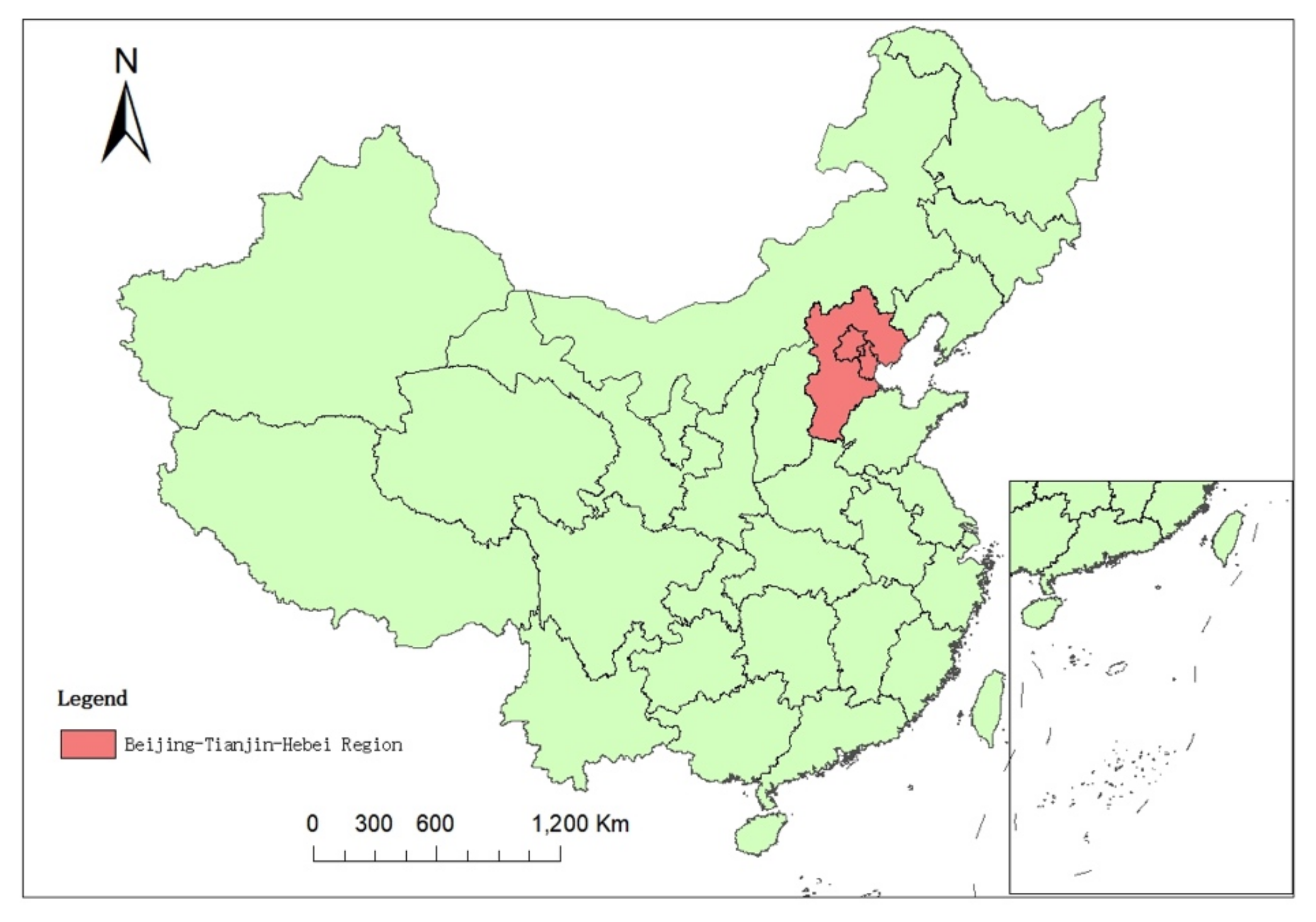
3.1. Study Area

The BTH region was selected as the study area. Figure 1 shows the geographical location of Beijing, Tianjin, and Hebei in China.

3.2. Data Sources

The data sources include NTL data: DMSP/OLS and NPP/VIIRS. At the pixel scale, the spatial resolution was 1km × 1km. Lambert Azimuthal Equal Area Projection was employed in ArcGIS. Statistical data: population, industry and area, in terms of city scale (including Beijing, Tianjin, Shijiazhuang, and other 13 cities). Descriptive information on the data sources are given in

Table 1. Description of the data sources.

Data	Data Description	Year	Source
DMSP/OLS	Annual stable night light data	1992–2013	National Oceanic and Atmospheric Administration National Geophysical Data Center (NOAA/NGDC)
NPP/VIIRS	Monthly night light data	2013, 2014, 2017, 2018	NOAA/NGDC
NPP/VIIRS	Annual night light data	2015, 2016	NOAA/NGDC
Boundaries	Shapefile of province	2015	National Geomatics Center of China
Population	Total regional population and urban population	1995, 2003, 2010, 2018	China City Statistical Yearbook Hebei Province 2010 population Census data
Industry	Proportion of the secondary industry in GDP Proportion of the tertiary industry in GDP	1995, 2003, 2010, 2018	China City Statistical Yearbook
Area	Urban area and construction land area	1995, 2003, 2010, 2018	China City Statistical Yearbook China Urban Construction Statistical Yearbook

.

3.3. Data Preprocessing

3.3.1. Integration of the Two NTL Datasets

1) Prior to the data fusion, the DMSP/OLS NTL data from 1992 to 2013 and the NPP/VIIRS NTL data from 2013 to 2018 were preprocessed:

(1) Monthly NPP/VIIRS data were averaged on an annual basis for 2013, 2014, 2017, and 2018. (2015 and 2016 were the annual data).

(2) Image reprojection, resampling, and cropping were performed on the two kinds of NTL data.

(3) In order to solve the problem of pixel saturation of DMSP/OLS data and lack of comparability of data pixels, the DMSP/OLS NTL data was mutually corrected and fused.

The invariant target area was selected as Jixi City in Heilongjiang Province for mutual image correction, which showed relatively stable economic and social development from 1992 to 2013 [39].

An annual fusion of NTL data obtained from different satellites during the same year was carried out to resolve the problem of varying NTL images produced by different satellites.

(4) Compared with the DMSP/OLS data, the NPP/VIIRS sensor can detect weaker lights with higher temporal and spatial resolution, but it does not remove sporadic weak lights such as flares, which will cause higher image noise. In order to reduce the influence of noise, this paper takes the stable bright element area of the 2016 annual synthetic data as the invariable area and makes stability corrections to the 2012–2016 data.

(5) Time series correction of two NTL data.

The basic assumption of the time series correction was consistent with the reality of China’s rapid economic development, that is, the pixel DN value of the NTL data from the previous year should not be greater than that in the following year.

2) Data fusion processing

Because the DMSP/OLS data covered 1992–2013, and the NPP/VIIRS data covered time since 2012, it was necessary to merge the two.

The fusion of the DMSP/OLS and NPP/VIIRS data was done following the literature [38], and county-scale DMSP/OLS data and NPP/VIIRS data for 2012 and 2013 were selected for regression fitting. A quadratic regression model was selected, and the fitting formula was given as shown in Equation (1). The R² of 0.8354 indicated a strong correlation between the two datasets.

$$f(x)=0.00003x^2+2.6539x+4726.5$$

(1)

where $x$ is the DMSP/OLS data in 2012 and 2013; $f(x)$ represents the NPP/VIIRS composite data for 2012 and 2013.

Equation (1) was used to perform the DMSP/OLS scale-continuity correction for the 2014–2018 NPP/VIIRS composite data, and the integrated NTL dataset was calculated to obtain the total DN values for China on the pixel scale from 1992 to 2018 (Figure 2).

In the ArcGIS software environment, the image was cut with a vector map mask on the BTH region to obtain NTL image data for the corresponding year. To avoid interference from the regional area, the average NTL values were selected for subsequent estimation of the urbanization level.

3.3.2. Preprocessing of Statistical Data

For population, industry, and area statistics in Table 1, the following calculations were performed:

$$x_1=\begin{array}{cc}urban& population/\begin{array}{ccc}total& regional& population\end{array}\end{array}$$

(2)

$$x_2=\begin{array}{cc}\sec ondary& industry\end{array}/GDP+\begin{array}{cc}tertiary& industry\end{array}/GDP$$

(3)

$$x_3=\begin{array}{ccc}construction& land& area\end{array}/\begin{array}{cc}urban& area\end{array}$$

(4)

The three indicators were standardized by min-max:

$$facto{r}_i=[x_i-\min (x_i)]/[\max (x_i)-\min (x_i)]$$

(5)

where $x_i$ is the original statistical data, which $facto{r}_i$ is the standardized data of the three urbanization factors, $i=1,2,3$.

3.4. Methodology and Model

3.4.1. Panel Entropy Weight Method

The entropy-weighting method is an objective method that has come into widespread use in recent years [40,41]. It is a method to determine the weight of indicators by using the amount of information provided by the entropy of various indicators. Entropy weighting method avoids the interference of human factors in the weight of each rating index and make the evaluation result more realistic. It overcomes the problem that the index weighting process is greatly affected by human factors in the current evaluation method. By calculating the entropy value of each index, it measures the size of the index information, to ensure that the established index can reflect most of the original information.

The smaller the entropy value of the factor, the greater the degree of variation in the factor value, the greater the amount of information provided, and the greater the weighting of the factor.

Assuming that the element number in the study area is $p$, the number of factors used is $q$, then the factor matrix is $p\times q$ The entropy of the $\begin{array}{cc}ith& factor\end{array}$ is defined as:

$$S_i=-(1/\ln p){\displaystyle {\sum }_{j=1}^p{y}_{ij}\ln y_{ij}}$$

(6)

where, $S_i$ is the entropy of the $\begin{array}{cc}ith& factor\end{array}$, and $p$ is the number of elements, $p=4\times 13$. When $y_{ij}=0$, $y_{ij}\ln y_{ij}=0$.

$y_{ij}$ is defined as:

$$y_{ij}=-M_{ij}/{\displaystyle {\sum }_{j=1}^p{M}_{ij}}$$

(7)

where $M_{ij}$ refers to the standardized factor value of the $\begin{array}{cc}ith& factor\end{array}$ and the $jth$ evaluation object.

The entropy weight of the $\begin{array}{cc}ith& factor\end{array}$ is defined as:

$${\omega }_i=(1-S_i)/{\displaystyle {\sum }_{i=1}^q(1-S_i)}$$

(8)

where, ${\omega }_i$ is the entropy weight of the $\begin{array}{cc}ith& factor\end{array}$, $0\le {\omega }_i\le 1$. $S_i$ is the entropy of the $\begin{array}{cc}ith& factor\end{array}$, ${\displaystyle {\sum }_{i=1}^q{S}_i}=1$. $q$ is the number of evaluation factors.

3.4.2. Construction of Composite Urbanization Index

The urbanization composite index is calculated according to the following formula:

$$U_p={\displaystyle {\sum }_{i=1}^3{\omega }_i\times x_i}$$

(9)

$U_p$ is the composite index of the urbanization level of $p$ element, $p=4\times 13$. ${\omega }_i$ is the weight of the $ith$ urbanization factor, $x_i$ is the population, industry, and area statistics, $i=1,2,3$.

3.4.3. Urbanization Level Estimation Model

The larger the DN value of the integrated NTL data, the larger the urbanization level. That is, the DN value has a close linear correlation to urbanization level at the pixel level. This study assumes that the correlation between DN and the municipal composite urbanization index is consistent at the pixel level.

Based on the integrated NTL datasets, the estimation model for urbanization level is established as follows:

$$U_p=aD{N}_p+b$$

(10)

where $U_p$ represents composite urbanization index at $p$ element, $D{N}_p$ represents $DN$ value at $p$ element, $a$ and $b$ were the parameters of the linear regression equation. Relying on the accuracy of urbanization level estimation model, the zero-error method of municipal composite urbanization index was adopted to correct the pixel-scale data.

3.4.4. Standard Deviational Ellipse

The standard deviation elliptical (SDE) method is a classical method of analyzing the directional characteristics of spatial distribution. The SDE has been used to analyze the spatial distribution of various phenomena in urban studies [42]. The existing research shows that the operation of SDE is simple and easy to be implemented in ArcGIS. More importantly, this technique is effective in exploring the spatial distribution of geographic events [43]. It is a good choice to employ SDE to study the spatial pattern of urbanization level of BTH in different periods.

The standard deviation ellipse can be utilized to explore the centrality, expansion, orientation, and spatial morphology of the spatial distribution of urbanization from the global and spatial perspectives. The specific calculation is as follows.

The form of the standard deviation ellipse is as follows:

$$SD{E}_x=\sqrt{{\displaystyle {\sum }_{i=1}^n(x_i-\overline{X})/n}}$$

(11)

$$SD{E}_y=\sqrt{{\displaystyle {\sum }_{i=1}^n(y_i-\overline{Y})/n}}$$

(12)

where $x_i$ and $y_i$ are the coordinates of elements, $\overline{X}$ and $\overline{Y}$ are the average central coordinates of the elements, and $n$ is the total number of elements.

The calculation method of rotation angle is as follows:

$$\tan \theta =(A+B)/C$$

(13)

$$A=({\displaystyle {\sum }_{i=1}^n{\overline{x_i}}^2}-{\displaystyle {\sum }_{i=1}^n{\overline{y_i}}^2})$$

(14)

$$B=\sqrt{{({\displaystyle {\sum }_{i=1}^n{\overline{x_i}}^2}-{\displaystyle {\sum }_{i=1}^n{\overline{y_i}}^2})}^2+4{({\displaystyle {\sum }_{i=1}^n\overline{x_i}\overline{y_i}})}^2}$$

(15)

$$C=2{\displaystyle {\sum }_{i=1}^n(\overline{x_i}-\overline{y_i})}$$

(16)

where $\overline{x_i}$ and $\overline{y_i}$ are the difference between the mean center and coordinates of $XY$.

The standard deviations of the $X$ and $Y$ axes are as follows:

$${\sigma }_x=\sqrt{2}\sqrt{{\displaystyle {\sum }_{i=1}^n{(\overline{x_i}\cos \theta -\overline{y_i}\sin \theta )}^2/n}}$$

(17)

$${\sigma }_y=\sqrt{2}\sqrt{{\displaystyle {\sum }_{i=1}^n{(\overline{x_i}\sin \theta -\overline{y_i}\cos \theta )}^2/n}}$$

(18)

The SDE method quantitatively represents the spatial distribution characteristics of the urbanization level across the spatial distribution range of the ellipse and the basic parameters of the center, long axis, short axis, and azimuth. The distribution range of the standard deviation ellipse gives the main range of the spatial distribution of the urbanization level.

3.4.5. Slope Analysis

Slope analysis [38] is to analyze the linear tendency of each pixel by using unitary linear regression model, which is widely used to analyze the year-over-year change of a certain variable. This study calculated the change in slope of the urbanization level from 1995 to 2018 by establishing an estimation model of the composite urbanization index. The changing trends of the urbanization level are analyzed on the county scale. The slope value was estimated using the least squares method, following the below formula:

$$Slope=(t\times {\displaystyle {\sum }_{i=1}^t{x}_i{U}_i}-{\displaystyle {\sum }_{i=1}^t{U}_i})/[t\times {\displaystyle {\sum }_{i=1}^t{x}_i^2}-{({\displaystyle {\sum }_{i=1}^t{x}_i})}^2]$$

(19)

where $t$ represents the total number of years, $x_i$ represents the $i$ year, and $U_i$ represents the urbanization level in $i$ year. For slope values greater than 0, the urbanization level showed an increasing trend. Slope values of less than 0, showed a decreasing trend in urbanization level.

4. Results and Analysis

4.1. Results of Estimated Urbanization Level Model

The panel data for the three selected urbanization level factors were established using the entropy weight method, and the entropy weights were 0.1772, 0.3119, and 0.5109, respectively. According to Equation (9) in 3.4.2, the composite index of the urbanization level was obtained:

$$U_p=0.1772x_1+0.3119x_2+0.5109x_3$$

(20)

where, $p=4\times 13$. $x_i$,$i=1,2,3$ is the population, industry, and area statistics.

The weighted composite urbanization index is shown in

Table 2. Statistical data of composite urbanization index.

City	1995	2003	2010	2018
Beijing	42.83586708	44.12330301	46.19424016	46.44189405
Tianjin	39.1717437	40.33985379	44.84089526	45.6840645
Shijiazhuang	30.52851942	33.23898604	37.24963332	40.29386958
Chengde	29.00864089	30.39204313	33.21276146	34.8186483
Zhangjiakou	30.73215558	32.21081533	34.36349803	36.73212172
Qinhuangdao	30.98045962	34.37005881	35.48317535	37.87514109
Tangshan	29.74829888	30.98342744	37.34239546	40.19754383
Langfan	28.29250165	31.14170283	36.24597932	39.97001141
Baoding	27.42296583	29.08140511	33.64952497	36.94346882
Cangzhou	28.24846267	29.78605488	34.96725626	38.57026499
Hengshui	26.30004851	28.79316136	31.8802259	36.42941843
Xingtai	26.85374076	28.69309943	33.70043723	37.11796903
Handan	28.67785202	29.33244091	34.93968266	38.47460702

The composite urbanization index and the mean values of the fused NTL data were used to establish the fixed-effects model between the indexes, as shown in Table 3.

.

The individual time-fixed-effects model was selected according to the results in

Table 3. Panel model estimation results.

Model	R2	p Value
Individual fixed effect	0.6235	0.0000
Time fixed effect	0.4542	0.0000
Individual-Time fixed effect	0.8808	0.0000

. The R² of the panel model was 0.8808, and the fitting precision was good. The fitting formula was follows:

$$U_p=0.4674D{N}_p+25.1508$$

(21)

where $U_p$ represents urbanization level at the municipal level, $D{N}_p$ represents the mean value at the municipal level. The estimated urbanization level values are shown in

Table 4. Composite urbanization index estimation data.

City	1995	2003	2010	2018
Beijing	31.59633396	35.99966943	42.06693432	46.41261372
Tianjin	32.49213349	37.31861211	44.39153457	50.67706861
Shijiazhuang	28.51925981	32.09996915	37.82508351	39.29358049
Chengde	25.34506489	28.34015601	33.46591146	31.86235431
Zhangjiakou	25.62876866	28.69817148	33.93738634	32.60681044
Qinhuangdao	26.94550993	30.39469229	36.24195472	36.70267697
Tangshan	28.83579543	33.10105927	39.85392413	42.70447061
Langfan	30.64245291	35.29534392	41.67849279	45.83009027
Baoding	27.24820319	30.79173107	36.37164656	36.75235562
Cangzhou	28.63288712	32.3295837	37.89207419	39.45089055
Hengshui	27.28773903	30.66211206	36.44620014	37.14309919
Xingtai	27.87361953	31.37194619	37.02403675	38.2188025
Handan	29.54985441	33.01772496	38.85199105	41.20646957

.

4.2. Accuracy Test of Estimated Model

Table 5. Relative estimation error (%).

City	1995	2003	2010	2018	Average RE (%)
Beijing	26.24%	18.41%	8.93%	0.06%	13.41%
Tianjin	17.05%	7.49%	1.00%	10.93%	9.12%
Shijiazhuang	6.58%	3.43%	1.54%	2.48%	3.51%
Chengde	12.63%	6.75%	0.76%	8.49%	7.16%
Zhangjiakou	16.61%	10.91%	1.24%	11.23%	10.00%
Qinhuangdao	13.02%	11.57%	2.14%	3.10%	7.46%
Tangshan	3.07%	6.83%	6.73%	6.24%	5.72%
Langfan	8.31%	13.34%	14.99%	14.66%	12.82%
Baoding	0.64%	5.88%	8.09%	0.52%	3.78%
Cangzhou	1.36%	8.54%	8.36%	2.28%	5.14%
Hengshui	3.76%	6.49%	14.32%	1.96%	6.63%
Xingtai	3.80%	9.34%	9.86%	2.97%	6.49%
Handan	3.04%	12.56%	11.20%	7.10%	8.48%

shows the relative errors and the average relative errors of 13 cities in the estimation model across four years. Among the relative errors, only the estimate for Beijing in 1995 exceeded 25%, indicating an overestimated urbanization level for Beijing in 1995. The average relative errors for the 13 cities were all less than 25%, indicating a good estimation accuracy for the model.

The overall city precision percentage is shown in

Table 6. Precision percentages for cities.

Year	Number of Cities			Precision Percentage (%)
	RE < 25%	RE (25~50%)	RE > 50%	High	Middle	Low
1995	12	1	0	92.3%	7.7%	0
2003	13	0	0	100%	0	0
2010	13	0	0	100%	0	0
2018	13	0	0	100%	0	0

.

There were 12, 13, 13, and 13 cities with a relative error of less than 25%, accounting for 92.3%, 100%, 100%, and 100% of the total precision in 1995, 2003, 2010, and 2016 respectively. The average estimation accuracy of more than 98% was relatively high, and the precision of the urbanization level estimation model on the municipal level met the requirements.

4.3. Spatiotemporal Dynamics of Urbanization Level

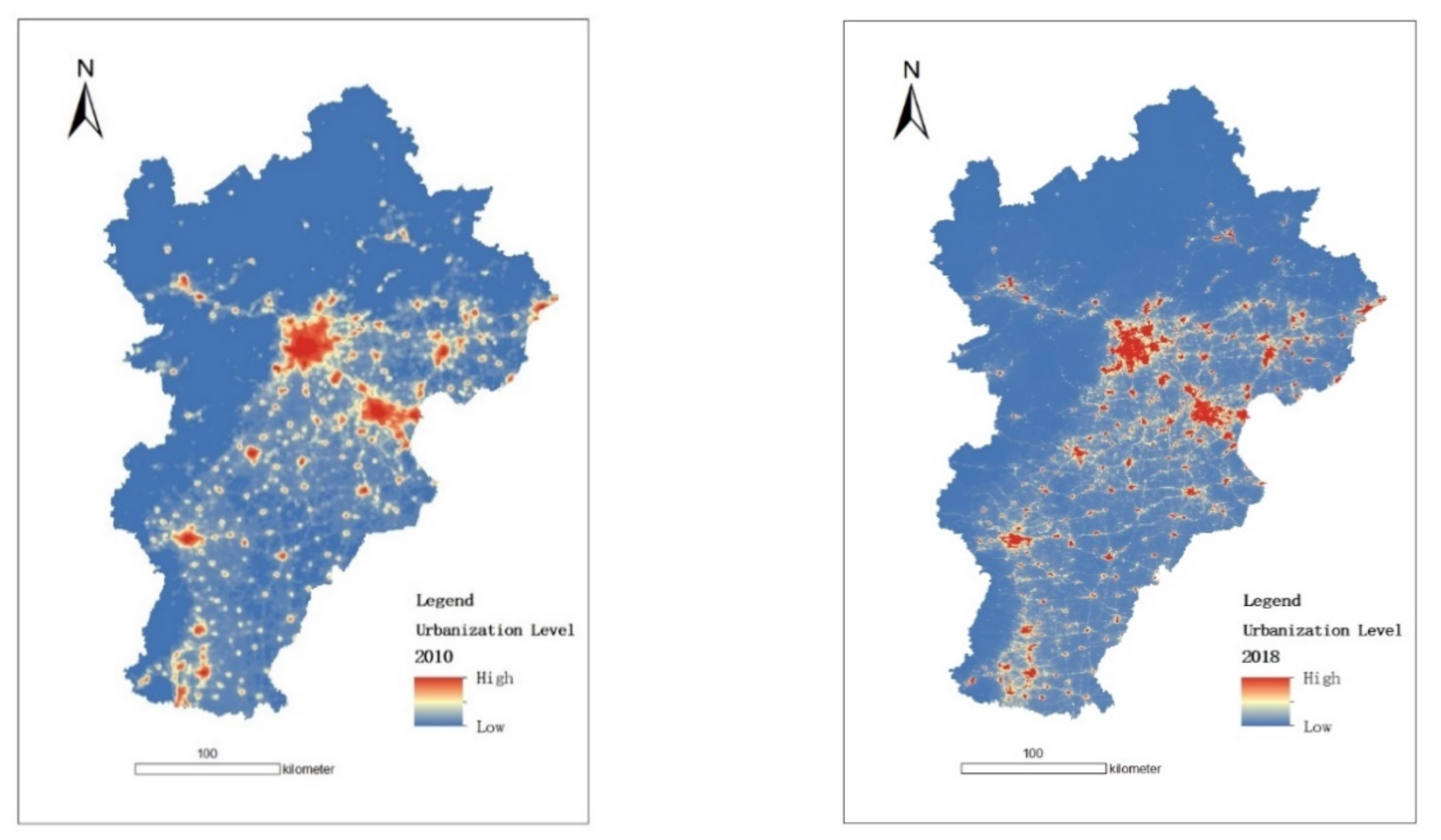
4.3.1. Spatiotemporal Dynamics from Pixel Scale

Figure 3 plots that, from 1995 to 2018, the overall urbanization level of BTH was strengthened. Areas with high levels of urbanization were obviously concentrated in the city centers of BTH. Areas with low levels of urbanization were distributed across in Baoding, Chengde, and Zhangjiakou and were concentrated in the northwestern part of the BTH region in an inverted “L” shape. After this fusion, the characteristics of NTL data distribution in the BTH region were more consistent with the differences in the urbanization process.

4.3.2. Spatiotemporal Dynamics on a Municipal Scale

As shows in Figure 4, from 1995 to 2003, the urbanization level of Langfang City rose from a higher to the highest level, and that of Tangshan City and Handan City rose from a medium to a higher level. The changes in Langfang and Tangshan reflected the way that Beijing and Tianjin drove the development of neighboring provinces and cities. From 2003 to 2010, overall urbanization did not significantly change. From 2010 to 2018, the urbanization of Xingtai City rose from a lower to a medium level.

Overall, from 1995 to 2018, the level of urbanization in BTH grew. High-level urbanization areas throughout this period were always concentrated near Beijing and Tianjin (Langfang City and Tangshan City were added in 2003), while low-level areas were always concentrated in Chengde City and Zhangjiakou City in the Hebei Province.

Figure 5 shows the spatiotemporal evolution of the standard deviation ellipse from 1995 to 2018.

Table 7. Each parameter value in the standard deviation ellipse.

Year	CenterX	CenterY	XstdDist	YstdDist	Rotation
1995	956848.1085	4245192.0137	121004.6673	247322.4747	27.7723
2003	957388.5857	4245606.6707	120775.5151	246554.2926	27.8991
2010	957861.0030	4245882.5435	120878.2018	246553.5045	28.0285
2018	958990.2015	4244356.3494	118682.5406	244520.6538	28.4747

presents changes in various parameters in the standard deviation ellipse from 1995 to 2018. Among them, Center X and Center Y represent the center points of the ellipse. XstdDist and YstdDist represent the length of the X axis and the length of the Y axis. Rotation represents the direction angle of the ellipse.

In reference to spatial rotation changes, the rotation value rose from 27.7723 in 1995 to 27.8991 in 2003 and then from 28.0285 in 2010 to 28.4747 in 2018. The direction of the generated ellipse is basically consistent with the spatial and temporal distributions of the high-level urbanization area in BTH. During the study period, the central movement path of the spatial distribution pattern of the high-level urbanization area in BTH showed a trend toward the northeast, from 1995 (956848.1085, 4245192.0137) to 2018 (958990.2015, 4244356.3494). The long semi-axis decreased from 247322.4747 in 1995 to 244520.6538 in 2018, and the short semi-axle decreased from 121004.6673 in 1995 to 118682.5406 in 2018.

The magnitude of the decline indicates that areas of high-level urbanization are increasingly concentrated in the main directions around Beijing and Tianjin.

From 1995 to 2018, the ellipse-flattening rate increased year-over-year, such that the spatial distribution pattern of the urbanization level of BTH still radiated and diffused its influence from Beijing-Tianjin to the periphery, especially toward the northeast. However, the spread of this influence shows tightening trend, and it is strengthening year-over-year.

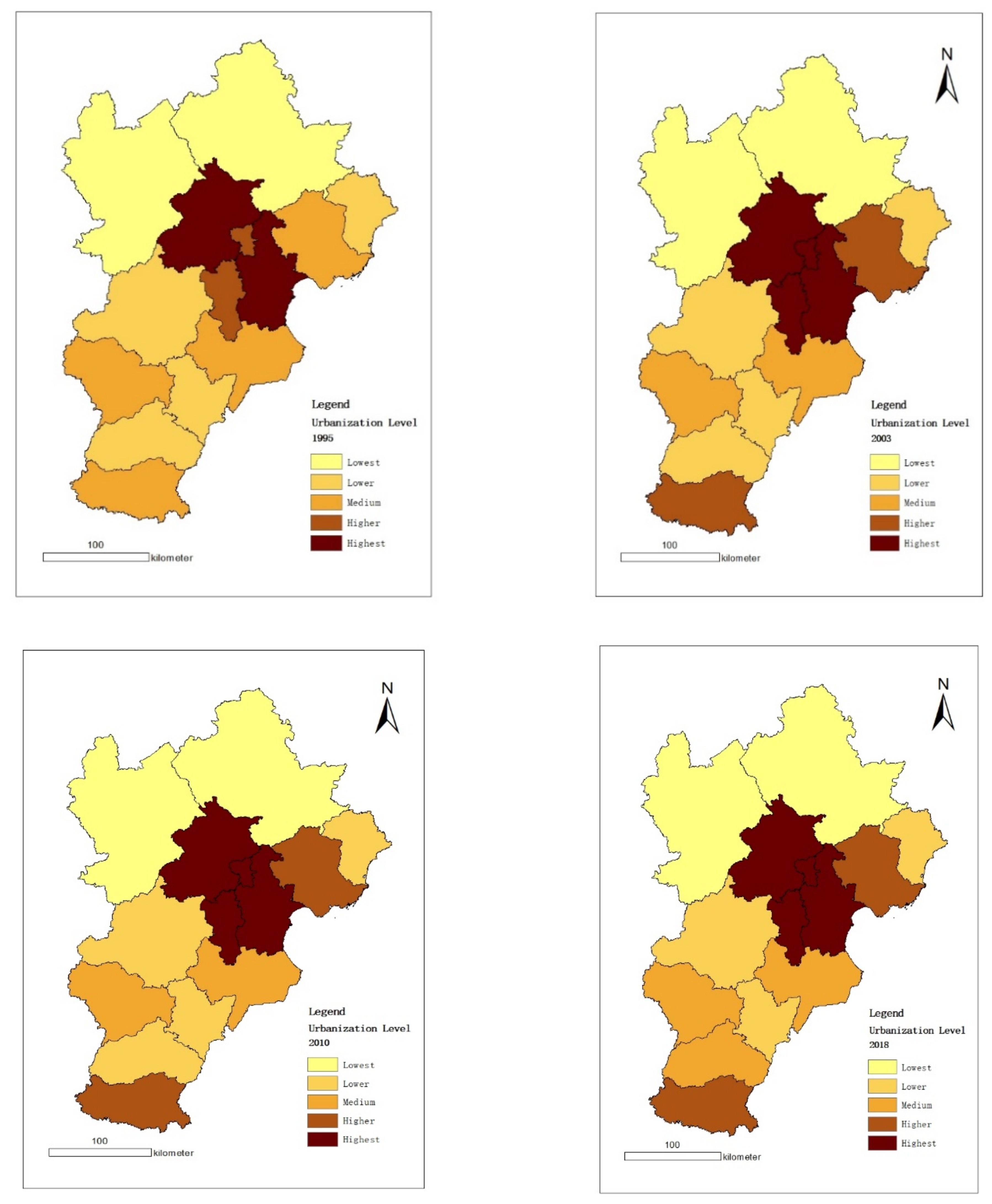
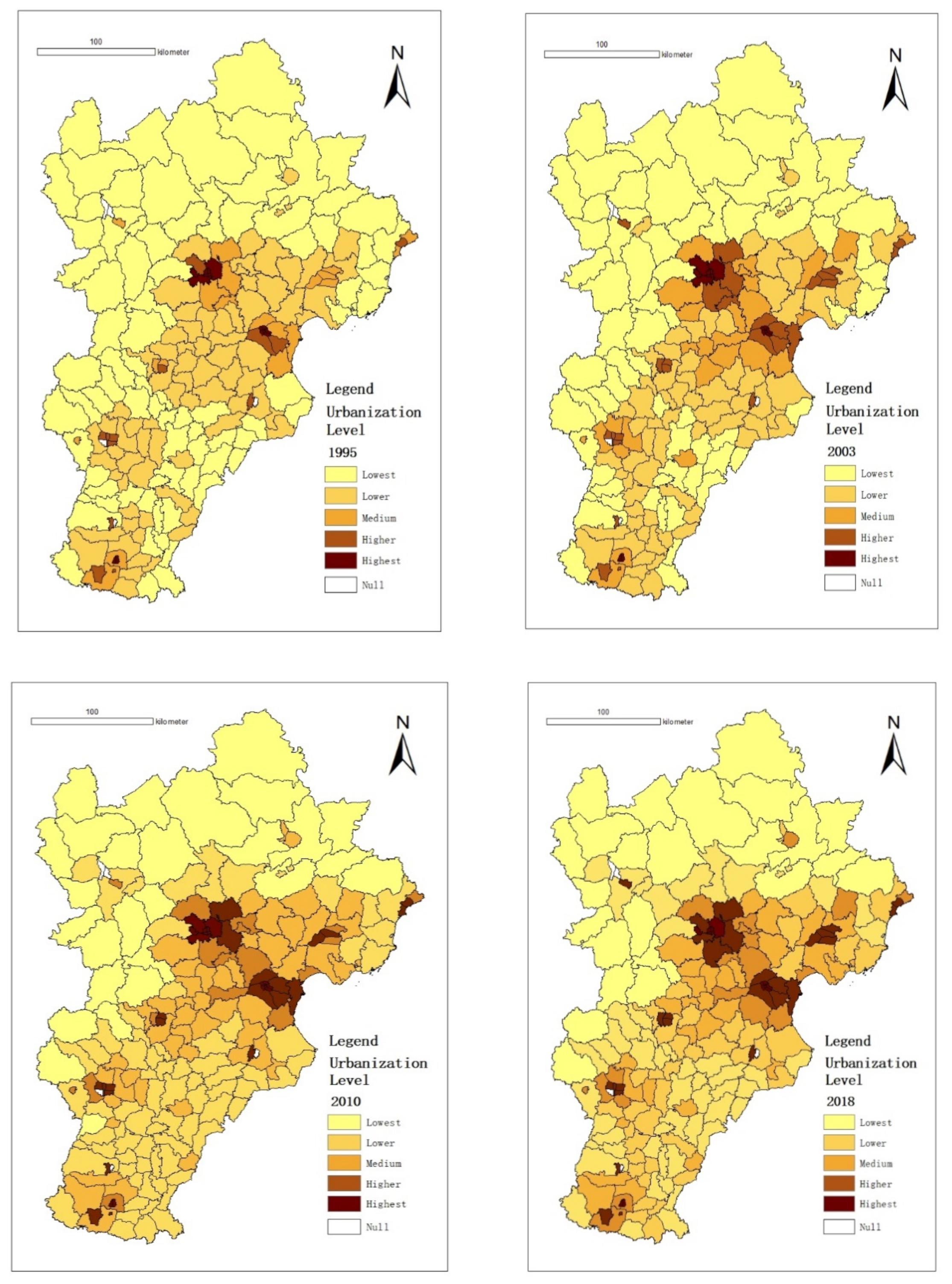
4.3.3. Spatiotemporal Dynamics from County Scale

(1)

Overall change trend in urbanization level at the county scale in BTH

From 1995 to 2018, county-scale urbanization levels in the BTH region showed a rapid growth trend, as indicated in Figure 6. In 1995, the areas with the highest level of urbanization were concentrated in Xicheng District, Dongcheng District, Xuanwu District, Chongwen District, Chaoyang District, Shijingshan District, and Fengtai District in Beijing; Hongqiao District, Nankai District, Hebei District, Hexi District, Heping District, and Hedong District in Tianjin City; and Fuxing District and Congtai District of Handan City, Hebei Province. The highest-level urbanization was concentrated in urban centers with dense populations, developed economies, and high energy consumption.

The highest-level urbanization areas newly added in 2018 were Haidian District, Shunyi District, Tongzhou District, and Daxing District in Beijing City; Beichen District, Dongli District, Xiqing District, Jinnan District, and Tanggu District in Tianjin City; and 18 counties in the Hebei Province, including Xinhua District, Qiaodong District, Chang’an District, Yuhua District in Shijiazhuang City, Guzhi District, Kaiping District, Lunan District, and Lubei District in Tangshan City. The range of highest-level urbanization spread from the urban center of each city to the surrounding areas.

From 1995 to 2018, the areas with the lowest level of urbanization were concentrated in Zhangjiakou City, Chengde City, and Qinglong Manchu Autonomous Region in Qinhuangdao City, as well as counties in the northwestern part of Baoding City. They were distributed in an L shape on the northwestern edge of BTH.

The spatiotemporal development of the urbanization in each city presents the characteristics of point-piece-flat evolution. Although the level of urbanization in most regions remains below the middle level, compared with 1995, the scope has greatly expanded, covering almost the entirety of the central and southern regions.

(2)

Number of counties above the medium level

As shown in Figure 7, from 1995 to 2018, the number of highest-level urbanization counties has been increasing in BTH. The reason for the instability of the number of higher-level and medium-level counties is that the urbanization level of some counties at this level has increased (rather than decreased).

As shown in Figure 8, from 1995 to 2018, the cities with a significant increase in the number of counties above the medium level were Shijiazhuang City, Tangshan City, Handan City, and Langfang City. In Baoding City and Qinhuangdao City, the number of counties above the medium level rose from one in 1995 to three in 2018. The number of counties at this level in Chengde City and Zhangjiakou City rose from zero in 1995 to one in 2018. The number of counties in Xingtai City and Cangzhou City remained one, while there were zero in Hengshui City.

It is worth noting that although the number of counties above the medium level in Zhangjiakou City and Chengde City featured an increasing trend from 1995 to 2018, few counties were above the medium level. Similarly, in Xingtai City, Cangzhou City, and Hengshui City, the overall level of urbanization was low.

(3)

Number of lowest-level counties

As shown in Figure 9, the number of counties with the lowest levels of urbanization in Beijing City and the Hebei Province showed a downward trend, with the fastest decline between 2003 and 2010. The number of counties with the lowest level of urbanization in Tianjin City remained zero.

In Figure 10, it can be seen that from 1995 to 2018, zero counties had the lowest-level urbanization in Langfang City. In Tangshan City, Handan City, Xingtai City, Cangzhou City, and Hengshui City the number of counties with the lowest level of urbanization fell to zero between 1995 and 2018. In Shijiazhuang City and Qinhuangdao City, the number fell to one. In addition, Baoding City, Zhangjiakou City, and Chengde City had a large number of counties with the lowest urbanization level in 2018, especially Zhangjiakou City and Chengde City.

(4)

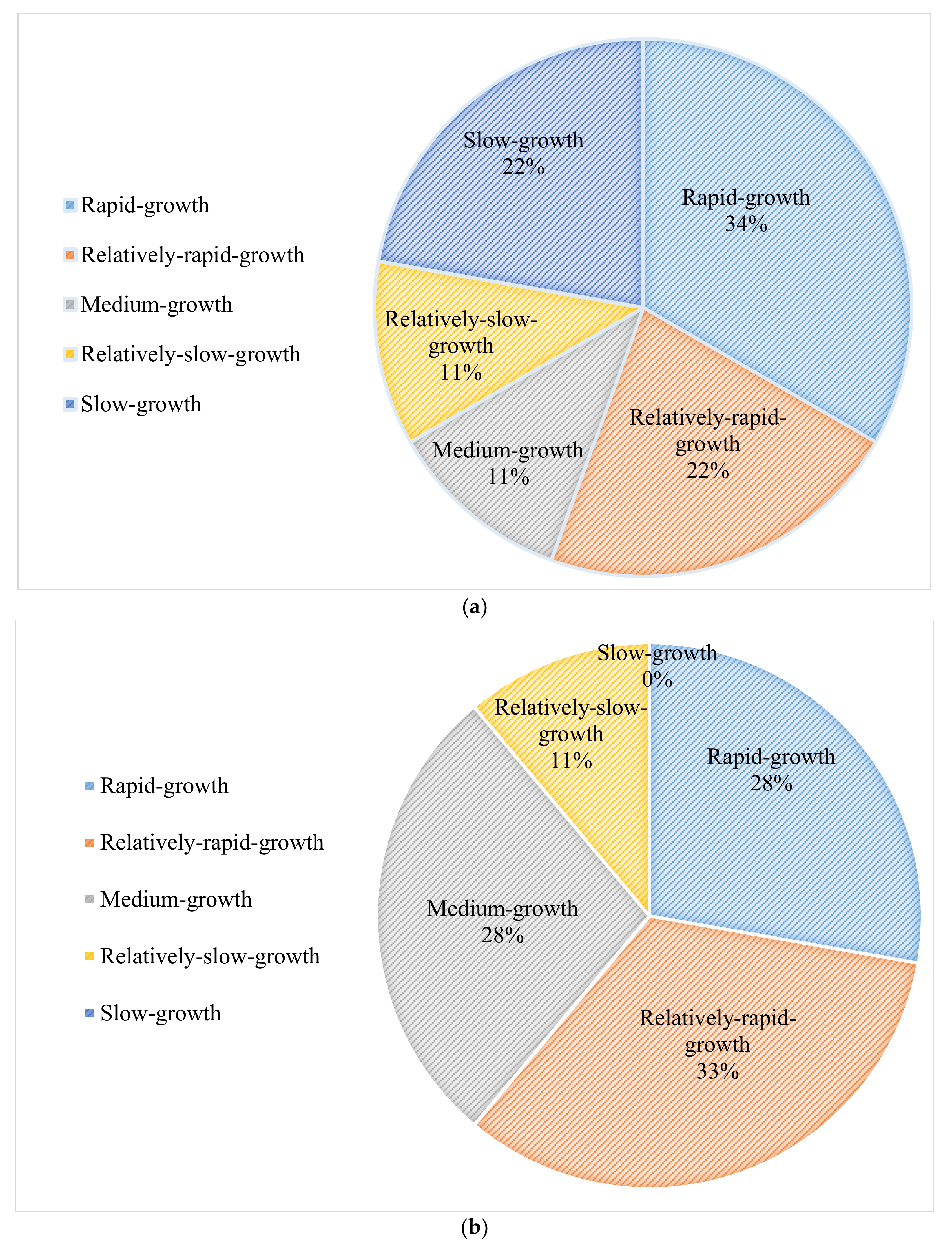
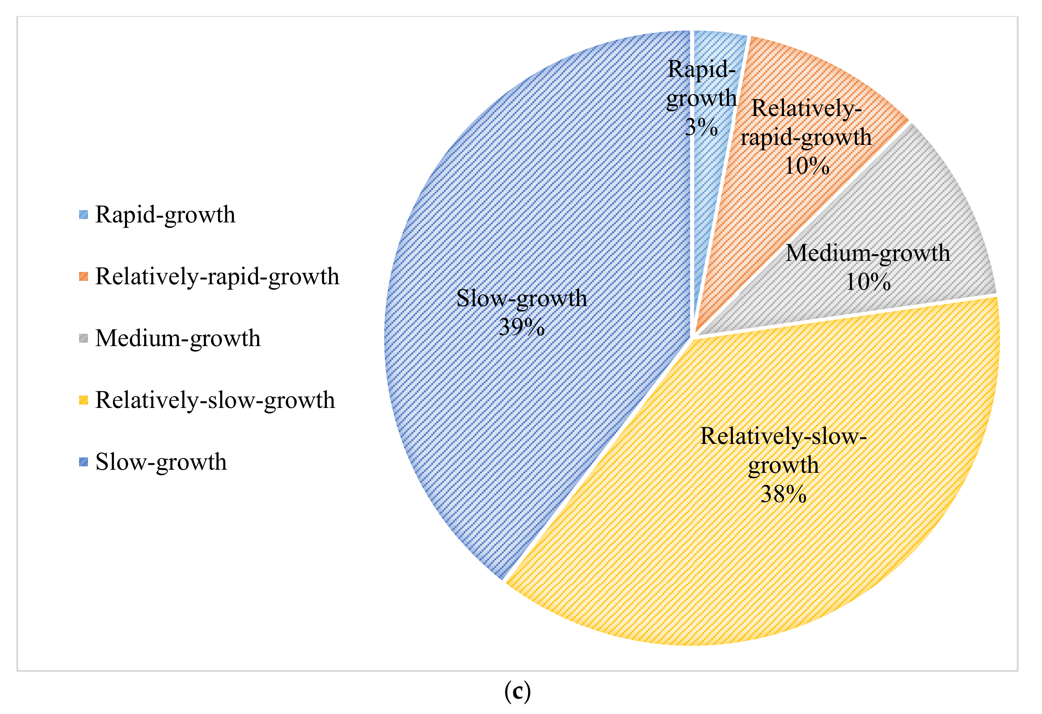
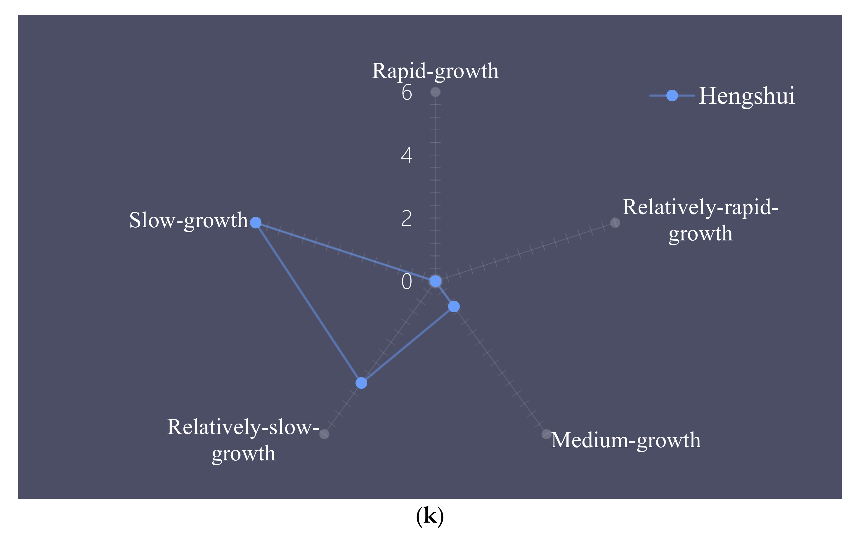
Growth rate of urbanization level at the county scale

To further explore the growth rate in urbanization for each county in the BTH region from 1995 to 2018, a slope analysis of the estimated urbanization level for 24 consecutive years from 1995 to 2018 was conducted. The slope results were divided into five groups, using the natural fracture method in ArcGIS. The specific groupings are given in

Table 8. Grading standards or urbanization level slopes.

Type	Slow Growth	Relatively Slow Growth	Medium Growth	Relatively Rapid Growth	Rapid Growth
Slope	<0.2145	0.2145–0.3450	0.3450–0.5520	0.5520–0.7936	>0.7936

.

Following the grouping in Table 8, the slopes are shown in Figure 11.

As shown in Figure 11, The rapid-growth regions are concentrated in the city centers of Beijing, Tianjin City, and certain prefecture-level cities in the Hebei Province (Yuhua District in Shijiazhuang City, Lunan District in Tangshan City, Beidaihe District in Qinhuangdao City, Congtai District in Handan City, and Nancheng District in Baoding City). In general, the urbanization level of most counties in the Hebei Province grew only slowly. Figure 12 shows the proportion of counties corresponding to each growth level.

Figure 12 shows that more than half of districts in Beijing and Tianjin City had rapid growth and relatively rapid growth.

By contrast, the counties with rapid growth and relatively rapid growth only accounted for 13% of the Hebei province, and 77% of the counties in the urbanization growth rate were below medium growth.

In Figure 13, the slow growth and relatively slow growth counties were concentrated in Xingtai City, Baoding City, Zhangjiakou City, Chengde City, Cangzhou City, and Hengshui City, especially in Zhangjiakou City and Chengde City.

For Shijiazhuang City, Qinhuangdao City, and Handan City, different growth rates correspond to different numbers of counties, indicating that the urbanization development of these three cities was relatively unbalanced.

For Tangshan City and Langfang City, the number of counties was concentrated in relatively rapid growth, medium growth, and relatively slow growth, and the quantity gap among these was small, indicating that their urbanization development was relatively balanced.

4.4. Analysis and Discussion

Unlike the equal weighting in existing research [24,25], the composite urbanization index constructed by the panel entropy weighting can reflect the importance of each factor. On this basis, the urbanization level estimation model constructed had good results and high accuracy (Table 6). Limited by the availability of statistical indicators, the urbanization level estimation model can only perform accuracy testing on a city scale. However, as China’s statistical information improves, data at the county scale or smaller will continue to develop, allowing better scale model testing.

With this model, zero error correction on the pixel scale can be carried out on the fused NTL data. The corrected light map can represent the spatiotemporal evolution analysis of the urbanization level on the city or county scale. Fused NTL data can overcome the shortcomings of a single source such as short timelines and through zero-error correction at the pixel scale, so NTL data can be flexibly applied to the estimation of urbanization levels.

From 1995 to 2018, areas with high levels of urbanization in BTH were concentrated in Beijing, Tianjin, and the city centers of prefecture-level cities in the Hebei Province (Figure 3 and Figure 4). Urban areas with low levels of urbanization were concentrated in the northwestern part of the Hebei Province, distributed in an “L” shape on the northwestern edge of the BTH region, and these could be areas for subsequent urbanization work. Using standard deviation ellipse analysis (Figure 5, Table 7), it was found that the influence of Beijing and Tianjin on their surrounding areas is concentrated in the northeast, such as in Langfang and Tangshan, and the scope of their influence was shrinking year-over-year. This indicates that the scope of influence of Beijing and Tianjin’s ability to promote the development of the surrounding cities has been shrinking year-over-year. The number of counties with the highest level of urbanization in the three cities of BTH was increasing year-over-year (Figure 7), and the number of counties at the lowest level was decreasing year-over-year (Figure 9). In general, urbanization was constantly improving in BTH. Combined with the results of slope analysis (Figure 12), Beijing and Tianjin were generally at higher levels of urbanization development, and more than 50% of the districts and counties were fast and relatively fast.

The number of counties in the Hebei Province is decreasing with the increase in level, showing a pyramidal distribution. High-level counties in the Hebei Province were mainly concentrated in Shijiazhuang City, Tangshan, Handan City, and Langfang City (Figure 8). Combined with a slope analysis (Figure 13a,b,d,j), the urbanization of Shijiazhuang and Handan was relatively unbalanced, while that of Tangshan and Langfang was relatively balanced.

Xingtai City, Cangzhou City, and Hengshui City featured a small number of counties above the medium level of development (Figure 8), and the number of counties with the lowest level of development was also small (Figure 10), indicating that the county level data were mostly concentrated in the lower and medium levels. Combined with slope analysis (Figure 13e,i,k), the urbanization development rate of these three cities was slow, reflecting a lack of momentum for urbanization development in these three cities, and targeted industries and policies are urgently needed to drive the development of urbanization.

Low-level counties in the Hebei Province were concentrated to the northwest of Baoding City, Zhangjiakou City, and Chengde City (Figure 10). Combined with slope analysis (Figure 13f,g,h), Baoding City, Chengde City and Zhangjiakou City showed a low level of urbanization and low growth rate overall, which can be a target for future development.

5. Conclusions and Suggestions

(1) The fixed-effects model showed that the composite urbanization index thus produced had a strong correlation with the fused NTL data. The urbanization level estimation model constructed had good results and high accuracy. The empirical results showed that after correction, it is appropriate to use night light data to indicate the level of urbanization. An effective attempt had been made for subsequent urban development research.

(2) All the results indicated that the urbanization levels of Beijing City and Tianjin City are both the highest and the fastest growing. The spatiotemporal results at the county level showed that the urbanization levels of Shijiazhuang City and Handan City are the highest in the Hebei Province. For these areas with high levels, the focus can be on how the quality of urbanization can be improved and how modern city construction can be carried out. It is necessary to give full play to the role of high-level urbanization in the surrounding areas and to promote the development of neighboring areas. However, slope analysis showed that the urbanization development of Shijiazhuang City and Handan City is not balanced. In the follow-up development, it is necessary to pay attention to their own balanced development and enable the fast-growing districts (counties) to drive the neighboring districts (counties) to achieve the coordinated development of the entire city.

(3) Both the results at city and county scales indicated that the urbanization level of Chengde City and Zhangjiakou City is at the lowest level. At the county scale a large number of counties where Baoding City was at the lowest level of urbanization. These areas are largely marginal areas of the BTH region. In the future, it is necessary to establish the dominant position of local cities, improve the level of infrastructure, optimize the industrial layout, enhance the attractiveness of the population, and improve the overall improvement of regional urbanization.

(4) Although the spatiotemporal results did not show that Xingtai City, Cangzhou City and Hengshui City are at low urbanization level, the slope results showed that the urbanization growth of these three cities is slow. The first task is to solve how to improve rapid urbanization, how to stimulate the vitality of urban development and narrow the gap with other cities. For example, technological innovation and industrial upgrading should be used to drive economic growth, stimulate domestic demand and then increase exports, increase labor rates, and thereby increase the level of urbanization.

(5) The spatiotemporal results at the county scale showed that the number of counties with the lowest levels of urbanization in Langfang City and Tangshan City are both zero. Slope analysis showed that the development of the two cities is relatively balanced. For Langfang City and Tangshan City, the urban construction plan should be reasonably planned to ensure the continuous and stable development of the city’s level of urbanization, and the quality of the urbanization level can be improved.

References

1. Bhatta, B.; Saraswati, S.; Bandyopadhyay, D. Quantifying the degree-of-freedom, degree-of-sprawl, and degree-of-goodness of urban growth from remote sensing data. Appl. Geogr. 2010, 30, 96–111. [Google Scholar] [CrossRef]
2. Clark, P.; Bairoch, P.; Braider, C. Cities and Economic Development from the Dawn of History to the Present. Econ. Hist. Rev. 1990, 43, 326. [Google Scholar] [CrossRef]
3. Yang, S.; Shi, L. Prediction of long-term energy consumption trends under the New National Urbanization Plan in China. J. Clean. Prod. 2017, 166, 1144–1153. [Google Scholar] [CrossRef]
4. Chen, M.; Liu, W.; Lu, D. Challenges and the way forward in China’s new-type urbanization. Land Use Policy 2016, 55, 334–339. [Google Scholar] [CrossRef]
5. Liu, Y.; Li, J.; Yang, Y. Strategic adjustment of land use policy under the economic transformation. Land Use Policy 2018, 74, 5–14. [Google Scholar] [CrossRef]
6. Zhao, Z.; Bai, Y.; Wang, G.; Chen, J.; Yu, J.; Liu, W. Land eco-efficiency for new-type urbanization in the Beijing-Tianjin-Hebei Region. Technol. Forecast. Soc. Chang. 2018, 137, 19–26. [Google Scholar] [CrossRef]
7. Tian, G.; Qiao, Z. Assessing the impact of the urbanization process on net primary productivity in China in 1989–2000. Environ. Pollut. 2014, 184, 320–326. [Google Scholar] [CrossRef]
8. Fan, J.-L.; Zhang, Y.-J.; Wang, B. The impact of urbanization on residential energy consumption in China: An aggregated and disaggregated analysis. Renew. Sustain. Energy Rev. 2017, 75, 220–233. [Google Scholar] [CrossRef]
9. Wu, Y.; Zhang, X.; Shen, L. The impact of urbanization policy on land use change: A scenario analysis. Cities 2011, 28, 147–159. [Google Scholar] [CrossRef]
10. Zhao, M.; Cheng, W.-M.; Zhou, C.; Li, M.; Huang, K.; Wang, N. Assessing Spatiotemporal Characteristics of Urbanization Dynamics in Southeast Asia Using Time Series of DMSP/OLS Nighttime Light Data. Remote Sens. 2018, 10, 47. [Google Scholar] [CrossRef] [Green Version]
11. Liang, C.; Penghui, J.; Wei, C.; Manchun, L.; Liyan, W.; Yuan, G.; Yuzhe, P.; Nan, X.; Yuewei, D.; Qiuhao, H. Farmland protection policies and rapid urbanization in China: A case study for Changzhou City. Land Use Policy 2015, 48, 552–566. [Google Scholar] [CrossRef]
12. Bilgili, F.; Koçak, E.; Bulut, Ü.; Kuloğlu, A. The impact of urbanization on energy intensity: Panel data evidence considering cross-sectional dependence and heterogeneity. Energy 2017, 133, 242–256. [Google Scholar] [CrossRef]
13. Cai, Z.; Liu, Q.; Cao, S. Real estate supports rapid development of China’s urbanization. Land Use Policy 2020, 95, 104582. [Google Scholar] [CrossRef]
14. Zhang, C.; Tian, H.; Chen, G.; Chappelka, A.; Xu, X.; Ren, W.; Hui, D.; Liu, M.; Lu, C.; Pan, S.; et al. Impacts of urbanization on carbon balance in terrestrial ecosystems of the Southern United States. Environ. Pollut. 2012, 164, 89–101. [Google Scholar] [CrossRef]
15. Wang, Y.; Zhao, T. Impacts of urbanization-related factors on CO 2 emissions: Evidence from China’s three regions with varied urbanization levels. Atmos. Pollut. Res. 2018, 9, 15–26. [Google Scholar] [CrossRef]
16. Lin, B.; Zhu, J. Changes in urban air quality during urbanization in China. J. Clean. Prod. 2018, 188, 312–321. [Google Scholar] [CrossRef]
17. Lin, X.; Wang, Y.; Wang, S.; Wang, D. Spatial differences and driving forces of land urbanization in China. J. Geogr. Sci. 2015, 25, 545–558. [Google Scholar] [CrossRef]
18. Zhang, W.; Wang, M.Y. Spatial-temporal characteristics and determinants of land urbanization quality in China: Evidence from 285 prefecture-level cities. Sustain. Cities Soc. 2018, 38, 70–79. [Google Scholar] [CrossRef]
19. Ju, Y.; Dronova, I.; Guo, Q.; Zhang, X. Analysis of urbanization dynamics in mainland China using pixel-based night-time light trajectories from 1992 to 2013. Int. J. Remote Sens. 2017, 38, 6047–6072. [Google Scholar] [CrossRef]
20. Dong, J.; Zhuang, D.; Xu, X.; Ying, L. Integrated Evaluation of Urban Development Suitability Based on Remote Sensing and GIS Techniques—A Case Study in Jingjinji Area, China. Sensors 2008, 8, 5975. [Google Scholar] [CrossRef] [PubMed]
21. Wang, X.; Wan, G. China’s Urban Employment and Urbanization Rate: A Re-estimation. China World Econ. 2014, 22, 30–44. [Google Scholar] [CrossRef]
22. Gu, C.; Guan, W.; Liu, H. Chinese urbanization 2050: SD modeling and process simulation. Sci. China Earth Sci. 2017, 14, 97–1082. [Google Scholar] [CrossRef]
23. Jin, G.; Deng, X.; Zhao, X.; Guo, B.; Yang, J. Spatiotemporal patterns in urbanization efficiency within the Yangtze River Economic Belt between 2005 and 2014. J. Geogr. Sci. 2018, 28, 1113–1126. [Google Scholar] [CrossRef] [Green Version]
24. Gao, B.; Huang, Q.; He, C.; Ma, Q. Dynamics of Urbanization Levels in China from 1992 to 2012: Perspective from DMSP/OLS Nighttime Light Data. Remote Sens. 2015, 7, 1721. [Google Scholar] [CrossRef] [Green Version]
25. Fu, H.; Shao, Z.; Fu, P.; Cheng, Q. The Dynamic Analysis between Urban Nighttime Economy and Urbanization Using the DMSP/OLS Nighttime Light Data in China from 1992 to 2012. Remote Sens. 2017, 9, 416. [Google Scholar] [CrossRef] [Green Version]
26. Elvidge, C.D.; Baugh, K.E.; Dietz, J.B.; Bland, T.; Sutton, P.C.; Kroehl, H.W. Radiance Calibration of DMSP-OLS Low-Light Imaging Data of Human Settlements. Remote Sens. Environ. 1999, 68, 77–88. [Google Scholar] [CrossRef]
27. Elvidge, C.D.; Baugh, K.E.; Anderson, S.J.; Sutton, P.C.; Ghosh, T. The Night Light Development Index (NLDI): A spatially explicit measure of human development from satellite data. Soc. Geogr. 2012, 7, 23–35. [Google Scholar] [CrossRef]
28. Zhou, Y.; Smith, S.J.; Elvidge, C.D.; Zhao, K.; Thomson, A.M.; Imhoff, M.L. A cluster-based method to map urban area from DMSP/OLS nightlights. Remote Sens. Environ. 2014, 147, 173–185. [Google Scholar] [CrossRef]
29. Zhao, J.; Ji, G.; Yue, Y.; Lai, Z.; Chen, Y.; Yang, D.; Yang, X.; Wang, Z. Spatio-temporal dynamics of urban residential CO2 emissions and their driving forces in China using the integrated two nighttime light datasets. Appl. Energy 2019, 235, 612–624. [Google Scholar] [CrossRef]
30. Lv, Q.; Liu, H.; Yang, D.; Liu, H. Effects of urbanization on freight transport carbon emissions in China: Common characteristics and regional disparity. J. Clean. Prod. 2019, 211, 481–489. [Google Scholar] [CrossRef]
31. Ma, T.; Zhou, Y.; Zhou, C.; Haynie, S.; Pei, T.; Xu, T. Night-time light derived estimation of spatio-temporal characteristics of urbanization dynamics using DMSP/OLS satellite data. Remote Sens. Environ. 2015, 158, 453–464. [Google Scholar] [CrossRef]
32. Zhang, Q.; Seto, K.C. Mapping urbanization dynamics at regional and global scales using multi-temporal DMSP/OLS nighttime light data. Remote Sens. Environ. 2011, 115, 2320–2329. [Google Scholar] [CrossRef]
33. Yi, K.; Tani, H.; Li, Q.; Zhang, J.; Guo, M.; Bao, Y.; Wang, X.; Li, J. Mapping and Evaluating the Urbanization Process in Northeast China Using DMSP/OLS Nighttime Light Data. Sensors 2014, 14, 3207. [Google Scholar] [CrossRef] [PubMed] [Green Version]
34. Zheng, Q.; Weng, Q.; Wang, K. Developing a new cross-sensor calibration model for DMSP-OLS and Suomi-NPP VIIRS night-light imageries. ISPRS J. Photogramm. Remote Sens. 2019, 153, 36–47. [Google Scholar] [CrossRef]
35. Shi, K.F.; Yu, B.L.; Huang, Y.X.; Hu, Y.J.; Yin, B.; Chen, Z.Q.; Chen, L.J.; Wu, J.P. Evaluating the Ability of NPP-VIIRS Nighttime Light Data to Estimate the Gross Domestic Product and the Electric Power Consumption of China at Multiple Scales: A Comparison with DMSP-OLS Data. Remote Sens. 2014, 6, 1705. [Google Scholar] [CrossRef] [Green Version]
36. Hu, Y.; Peng, J.; Liu, Y.; Yueyue, D.; Li, H.; Wu, J. Mapping Development Pattern in Beijing-Tianjin-Hebei Urban Agglomeration Using DMSP/OLS Nighttime Light Data. Remote Sens. 2017, 9, 760. [Google Scholar] [CrossRef] [Green Version]
37. Shi, K.; Huang, C.; Yu, B.; Yin, B.; Huang, Y.; Wu, J. Evaluation of NPP-VIIRS night-time light composite data for extracting built-up urban areas. Remote Sens. Lett. 2014, 5, 358–366. [Google Scholar] [CrossRef]
38. Lv, Q.; Liu, H.; Wang, J.; Liu, H.; Shang, Y. Multiscale analysis on spatiotemporal dynamics of energy consumption CO2 emissions in China: Utilizing the integrated of DMSP-OLS and NPP-VIIRS nighttime light datasets. Sci. Total. Environ. 2020, 703, 134394. [Google Scholar] [CrossRef]
39. Liu, Z.; He, C.; Zhang, Q.; Huang, Q.; Yang, Y. Extracting the dynamics of urban expansion in China using DMSP-OLS nighttime light data from 1992 to 2008. Landsc. Urban Plan. 2012, 106, 62–72. [Google Scholar] [CrossRef]
40. Chen, T.; Jin, Y.; Qiu, X.; Chen, X. A hybrid fuzzy evaluation method for safety assessment of food-waste feed based on entropy and the analytic hierarchy process methods. Expert Syst. Appl. 2014, 41, 7328–7337. [Google Scholar] [CrossRef]
41. Wang, T.; Chen, J.; Wang, T.; Wang, S. Entropy weight-set pair analysis based on tracer techniques for dam leakage investigation. Nat. Hazards 2014, 76, 747–767. [Google Scholar] [CrossRef]
42. Wong, D.W. Formulating a General Spatial Segregation Measure. Prof. Geogr. 2005, 57, 285–294. [Google Scholar] [CrossRef]
43. Zhang, P.; Lin, H.; Chitty, N.; Cao, K. Beijing temples and their social matrix—A GIS reconstruction of the 1912–1937 social scape. Ann. GIS 2016, 22, 129–140. [Google Scholar] [CrossRef]
Figure 1. Geographical location of Beijing, Tianjin, and Hebei in China.
Sustainability 13 02000 g001
Figure 2. National total DN values on the pixel scale from 1995 to 2018.
Sustainability 13 02000 g002
Figure 3. Urbanization level at the pixel scale.
Sustainability 13 02000 g003aSustainability 13 02000 g003b
Figure 4. Urbanization level at the municipal scale.
Sustainability 13 02000 g004
Figure 5. Standard deviation ellipse from 1995 to 2018.
Sustainability 13 02000 g005
Figure 6. Urbanization level at the county scale.
Sustainability 13 02000 g006
Figure 7. The number of counties above medium level in BTH.
Sustainability 13 02000 g007
Figure 8. Number of counties above the medium level in 11 cities in the Hebei Province.
Sustainability 13 02000 g008
Figure 9. Number of counties at lowest-level urbanization in BTH.
Sustainability 13 02000 g009
Figure 10. Number of counties at lowest-level urbanization in 11 cities in the Hebei Province.
Sustainability 13 02000 g010
Figure 11. Slope analysis of urbanization level on the county scale.
Sustainability 13 02000 g011
Figure 12. Proportion of counties with different growth levels in BTH. (a) Beijing City; (b) Tianjin City; (c) Hebei Province.
Sustainability 13 02000 g012aSustainability 13 02000 g012b
Figure 13. Radar maps of 11 cities in the Hebei Province. (a) Shijiazhuang City; (b) Tangshan City; (c) Qinhuangdao City; (d) Handan City; (e) Xingtai City; (f) Baoding City; (g) Zhangjiakou City; (h) Chengde City; (i) Cangzhou City; (j) Langfang City; (k) Hengshui City.
Sustainability 13 02000 g013aSustainability 13 02000 g013bSustainability 13 02000 g013cSustainability 13 02000 g013dSustainability 13 02000 g013e