Abstract
The mean-variance (MV) portfolio optimization targets higher return for investment period despite the unknown stochastic behavior of the future asset returns. That is why a risk is explicitly considering, quantified by algebraic characteristics of volatilities and co-variances. A new probabilistic definition of portfolio risk is the Value at Risk (VaR). The paper makes explicit inclusion and minimization of VaR as a quantitative measure of financial sustainability of a portfolio problem. Thus, the portfolio weights as problem solutions will respect not only the MV requirements for risk and return, but also the additional minimization of risk defined by VaR level. The portfolio problem is defined in a new, bi-level form. The upper level minimizes and evaluates the VaR value. The lower level evaluates the optimal assets weights by minimizing portfolio risk and maximizing the return in MV form. The bi-level model allows to have extended set of portfolio solutions with the portfolio weights and the value of VaR. Graphical interpretation of this bi-level definition of the portfolio problem explains the differences with the MV portfolio definition. Thus, the bi-level portfolio problem evaluates the optimal weights, which makes maximization of portfolio return and minimization of the risk in its algebraic and probabilistic form of definition.
1. Introduction
The financial sustainability is always important qualitative criterion for investors and business managers. The paper places the topic of sustainability in a narrow framework for the domain of portfolio management and optimization of financial investments. Despite its qualitative meaning, the sustainability in the different domains uses appropriate parameters, which estimates quantity levels of the sustainability. Thus, for the domain of portfolio management, this paper applies the level of risk as appropriate level of portfolio sustainability. The added value in this research derives formal quantification for the sustainability by the usage of the portfolio risk in the investment. In portfolio theory, two main criteria can be applied as parameters for the quantification of the portfolio sustainability: portfolio return and portfolio risk. However, the investment portfolio policy requires that, at first, low level of risk has to be achieved and thereafter—higher level of return. That is the reason the financial organization and business entities need to consider the financial sustainability as a mandatory prerequisite for planning and performing investments and/or business solutions. In an explicit quantitative way, the financial sustainability is not considered as a formal set of relations in many optimization problems. Particularly, in portfolio problems, the portfolio sustainability can be formalized quantitatively as the level of risk or potential losses, which the investment can have. This research uses the portfolio risk as a main parameter, which defines the level of the sustainability in portfolio optimization.
The formal developments of the modern portfolio theory follow the inclusion of different parameters and relations, which are included in portfolio problems. Starting with quantification of the assets characteristics mean returns and covariance matrix of the assets returns of the portfolio problem was complicated from its mean-variance (MV) background. Different types of returns were introduced like “current values” [1], “mean values” [2] and “implied values” [3]. Two general forms of risk category currently are exploited in the portfolio theory: ‘’variance/covariance” between the asset returns [2] and the probability nature of the risk as “Value at Risk” (VaR) and its derivatives as Conditional VaR [4]. Behind these portfolio parameters, there are a derived set of relations, originated by the MV approach [2], Capital Asset Pricing Model (CAPM) [1], Black-Litterman (BL) model, which includes subjective assessments for the modification of the assets parameters [3,5]. The benefit of the Modern Portfolio theory concerns the definition of appropriate portfolio optimization problem, giving the solution of the components of the investment to be allocated for assets positions by means to achieve in the investment horizon which is a tradeoff between the maximization of the portfolio return and minimization of the portfolio risk. The portfolio problem can have different structure and computational nature: static for one period of investment; dynamic for multi-period of optimization; with linear or nonlinear and/or integer relations. These forms of the portfolio problem apply only one goal function, formalizing the targets of the portfolio optimization. As a prospective form of optimization, a hierarchical, multilevel and particularly bi-level optimization is under extensive developments for usage in different application domains [6]. The practical implications of the bi-level portfolio formalization result in increase of the portfolio parameters, which are evaluated on their optimal values. For the case of the portfolio risk, this means that the bi-level approach will find optimal value of the portfolio risk as variance of the asset returns but simultaneously as optimal value of the probabilistic form of the risk, given by the parameter VaR. Such integration and optimal evaluation of both important characteristics of portfolio risk is a prerequisite for considering stable sustainability in the portfolio optimization.
This paper makes usage of this more complicated model of optimization in the portfolio theory. It defines two different goal functions, which are optimized on different hierarchical levels of the portfolio problem. The added value of this research is the introduction of the probability form of portfolio risk, VaR, as an argument of the goal function in a portfolio problem. Thus, the parameter VaR becomes a solution of the portfolio problem together with the weights of assets. Its value is optimal and this case differs when VaR participates as predefined value as a constraint in the portfolio problem.
2. Overview of Analytic Relations Used in the Portfolio
2.1. Improvement of the Portfolio Problem with Additional Constraints
The classical portfolio problem launched by [2] has mathematical programming form for minimization of the portfolio risk under the constraints of predefined value of return:
where wT = (w1, …, wN) is the solution of the portfolio problem and wi is the relative part of the investment, allocated for buying asset i, i = 1, N—the set of assets, participating in the portfolio; Σ—covariance matrix of the asset returns; ET = (E1, …, EN) mean returns of the assets; Edef is the required level of portfolio return.
Relation requires all the investment amount of resources to be allocated to the portfolio assets.
The problem (1) is the backbone over which complications and improvements are made to incorporate additional market parameters, participating to the investment process [7]. The most used forms of relations are additional constraints to the optimization problem. These constraints take into account requirements like:
Buy in threshold constraints [8]. These kinds of constraints prevent investors from holding small active positions. The smaller amount of assets shares impacts the portfolio performance in a very limited way. Such constraints are formalized by the integer inequality:
where is a prescribed proportion of the available capital; are additional binary variables, taking value 1 if investor buys shares of asset i, .
Round lot purchasing constraints. The institutional investors prefer to purchase blocks of individual financial assets. The preference comes from the case that trades with blocks which is easier than a smaller set of holdings. These forms of constraints are inequalities like:
where is integer variable and M is the amount of blocks.
Diversification constraints. They make limitations on the exposure to risky investments. Upper bounds on the maximum percentage of the portfolio are put on a certain level with integer variables The value holds if a set of assets is above a predefined level of investment resources and lower from upper bound:
Cardinality constraints [9]. They define the number of sectors in which the portfolio has to diversify the investment:
Value constraint [10]. This is a simplified form for limitation asset i to take less of percent of the total portfolio:
Limitation on changes in individual positions. This type of constraint can be formalized with upper and lower bounds:
Transactional costs. They are proportional to the asset weights:
where are the costs for buying/selling asset i. This value decreases the portfolio performance and can be included for the evaluation of the portfolio return . If relations (2)–(6) are added to the portfolio problem (1), the last becomes a nonlinear integer mathematical programming one. Such kinds of problems are computationally overloaded, which is an obstacle for decision making in limitation of time [11]. Difficulties accompanying the solution of complex portfolio problem are discussed in [12,13]. The portfolio problem is regarded as a single objective mean-variance one, which has mathematical form of convex integer quadratic programming with a set of constraints. The last formalizes additional financial requirements, which are met for the definition and implementation of the portfolio investment. Robust and probabilistic enhancements are discussed as prospective potential of the portfolio problem to formalize additional investment requirements. In another study [14], the portfolio problem is complicated by its application to multi-periods in investment. In another [15], the risk is formalized with high order moments of risk, which complicate computationally the portfolio problem. Comparisons of such modified MV portfolio problems are given in [16]. Attempt for extension of the portfolio problem with fuzzy formalizations is given in [17].
2.2. Mini-Max Definitions of the Portfolio Problem
Internally, the portfolio optimization problem targets minimization of the risk and simultaneously increases the portfolio return. This means that the portfolio problem has internal requirements to satisfy two contradictory goal functions. A formalization of the portfolio problem in mini-max definition has been developed. Another way of integrating these two contradictory goals is to use hierarchical multilevel optimization. The analysis, presented here, gives a picture that the attempts for the development of a usable hierarchical portfolio problem that is just beginning. Nevertheless, in this study [18], the term mini-max is used for the presentation of portfolio problem with uncertainty; this is not a hierarchically-ordered optimization problem. The mini-max terminology is applied for the definition of single goal optimization problem, where part of the uncertainty is minimized separately from the portfolio optimization and the computational workload insists finding a global optimum. The same case in single goal optimization is applied in [7,19]. A mini-max modeling portfolio is applied in [20]. It has been defined as a bi-linear optimization problem. The target of this problem is to find a tradeoff between the portfolio return and risk. In another study [21], the optimization portfolio problem is formalized in terms of game theory. Thus, min and max policies are implemented with mean-variance model. The defined problem minimizes the largest potential losses, which is the reason to apply the notation of mini-max problem.
Currently, a bi-level hierarchical approach is worked out for the design of an algorithm for solving portfolio problems with constraints about the CVaR (Conditional VaR) parameters [22]. The bi-level approach enters in modeling investment strategies in [23]. Bi-level modeling of portfolio MV problem is given in [24]. The bi-level programming framework is applied for the definition of a portfolio optimization problem [25]. The upper portfolio problem maximizes the Sharpe ratio and evaluates the assets weights as an upper level problem solution. The low level optimization problem minimizes the portfolio risk under given expected return. This bi-level formulation of the portfolio problem allows simultaneously to be maximized by the Sharpe ratio and to minimize the portfolio risk by the definition of the assets weights. Obviously, the portfolio problem has its internal content—the mini-max functionalities of its two important characteristics: risk and return. The simultaneous implementation of such contradictory goals currently is searched in a new complicated form of modeling by hierarchical bi-level optimization problems.
2.3. Other Forms of Risk Formalization
The traditional portfolio optimization, where the risk is quantified by the covariance between the asset returns is highly volatile. An alternative form of risk formalization is the model of Mean Absolute Deviation (MAD). This model is introduced in [26] for measuring the portfolio risk. A peculiarity of the portfolio problem, which applies MAD model is its linear programming form. The MAD model minimizes a measure of risk where the last is evaluated by the absolute mean return deviation. Formally, MAD evaluates the mean of the difference:
which theoretically is the same risk like MV model when the probabilistic distribution of the asset returns are normal [27]. MAD is easily calculated because it eliminates the estimation of the covariance matrix for the MV model. The portfolio problem of MAD is:
where Ei is the mean return of asset i; Ri is its current value.
MAD = E[|Ep−Rp|]
Thus, the MAD model equals to MV as one but the risk is substituted by the absolute deviation of portfolio return between its mean value Ep and the current portfolio return value Rp. This definition of the portfolio risk makes the optimization problem linear one, which is a prerequisite for its easier definition and solution.
Another form of the portfolio risk is introduced by probabilistic relations, which gives the models VaR (Value at Risk) and CVaR (Conditional VaR) of risk. This new measure of portfolio risk was developed by J.P. Morgan [28], later named Value at Risk. The risk is presented with probabilistic inequality, which characterizes the maximum likely loss for a predefined confidential interval. VaR has a duration chosen by the investor preferences for a day, month or another time horizon. The VaR estimation for a portfolio is currently widely acceptable for the risk management of a portfolio [29,30]. The probabilistic nature of VaR allows being overcome by the constraints of MV portfolio modeling and about the required normal distribution of the stochastic nature of assetreturns. Definition of analytic relations for the evaluation of VaR is given in [31]. Different algorithms for evaluation and optimization of VaR are presented in [32]. An additional way of usage of VaR in portfolio optimization, based on a non-parametric approach is given in [33]. The usage of VaR parameter for portfolio optimization is concerned in [34].
Thus, VaR can be used for different distribution laws, which is an advantage for such form of portfolio risk. In another study [35], comparison of using different definitions of risk as MAD, VaR and CVaR are given. The formal description of VaR is defined as integral of the density function of the stochastic portfolio profit:
where f(y) is the density function of a stochastic variable X (portfolio profit). VaR takes value γ, which is the maximum likely loss of the portfolio for the confidence interval [−∞, α]. The simplification of this integral relation is made by the usage of the cumulative probability function F(X). In Figure 1, the relations between the VaR parameters α and γ are given on the cumulative probability function F(X):
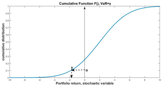
Figure 1.
VaR (Value at Risk) interpretation by cumulative distribution function.
The analytic relation for VaR is given by the probabilistic inequality:
Fx(γ) = Px (x ≤ γ) > α
The cumulative distribution function can take values from 0 to 1. Hence (10) can be presented also by the relation:
1 − Fx(γ) = Px (x > γ) ≤ 1 − α
The combination of (10) and (11) results into the well-known definition of VaR:
VaRα = inf{γ: P(x > γ) ≤ 1 − α} = inf{γ: Fx(γ) = α}
Hence, for the confidence level α, the maximum likely loss of the portfolio profit/return is VaRα = γ. If the inverse cumulative function F−1() is used, the VaR parameter can be expressed in the form:
VaRα = min{γ: F(γ) = α} = F−1(1 – α)
VaR measure is criticized because it does not respect sub-additive features, which makes VaR not a coherent risk measure. This means that the portfolio risk could be larger than the sum of risks of its components [36] or:
where is the risk of asset returns X and Y, and their combination X+Y. As a response for the sub-additive features of VaR, the modification Conditional VaR was introduced, which describes the risk measure in a bit of a different way [10]. Additional notations as “Expected short fall”, “Average VaR”, “Expected Tail Loss”, “super quantile” are also used instead of CVaR. The meaning of CVaR is analytically described like the definition of VaR. The last represents the integral part from the density probabilistic function f(X). Respectively, the CVaR integral part concerns the cumulative distributed function F(X):
Both relations (12) for VaR and (15) for CVaR are not algebraic ones and they have probabilistic nature. Such relations cannot be included directly in a portfolio optimization problem. For VaR and/or CVaR relations to be included in a portfolio problem, the general approach is to approximate the probabilistic relations with algebraic ones.
3. Approximation of VaR Relations
Following, the probabilistic inequality for VaR can be approximated in algebraic form. Using (10) and denoting Y as portfolio loss, it follows:
As the portfolio losses concern negative portfolio returns (16) becomes:
Describing the portfolio return as vector multiplication of the assets weights w and their stochastic asset returns R or –Y=RTw, (17) becomes:
where . For the inclusion of portfolio parameters E, w, Σ in relation to (18), the stochastic portfolio return process is normalized with mean zero and standard deviation equal to 1. Thus, (18) becomes:
Applying the equality relation (11), it holds:
The inverse function takes value for the percentage of the confidential interval. The current practice in investments uses values of the range = [90%, 95%, 99%]. Hence, the maximal loss can be optimized by the appropriate choice of the weights w of assets in the portfolio. The optimization goal function of the portfolio problem has to consider relation (19) by means to minimize VaR value for a given α.
In this work, it has been determined a bi-level optimization problem, which is defined by two interconnected optimization subproblems. The upper level optimization subproblem performs risk minimization, assuming VaR as a goal function derived in (19). The lower level subproblem solves a modification of the MV portfolio problem in the form:
Problem (20) targets minimization of the risk and simultaneously maximization of the return. The relative importance between the portfolio risk and return is given by the coefficient λ. By changing the value of λ, a series of portfolio problems are solved and their solutions belong to the “efficient frontier”. The bi-level optimization problem has a formal structure as:
Problem (21) applies the VaR relation (19) as goal function in a bi-level optimization. Hence, the solution w from (21) will simultaneously optimize three portfolio characteristics: VaR, Risk and Return from MV description. Respectively, the =VaR value will be minimal. In comparison with a MV problem (20), the last can optimize only two of them, Risk and Return from MV definition without VaR description of Risk. The extended set of optimized portfolio characteristics comes from the new, bi-level formalization of the portfolio problem.
4. Definition of a Bi-Level Portfolio Problem
The bi-level optimization is a prospective form for modeling and optimizing the management and control of systems in different practical domains [6]. The formal presentation of a bi-level problem is:
where the upper level subproblem is influenced by the solutions of the low level one. On its turn, the low level subproblem influences the upper one. For the portfolio case, the upper level will minimize the VaR loss γ and the lower level will optimize the portfolio Risk and Return, defined by MV model. Both upper and lower level subproblems will give optimal values of the assets weights w and γ. The analytical description of the low level modified MV subproblem (20) is the following:
By changing the solutions of (22) will give points of the efficient frontier . From the efficient frontier, an optimal solution is chosen, which gives maximal Sharpe ratio, defined as the ratio between the portfolio return and portfolio risk:
This MV portfolio will be compared with the solution of the bi-level problem, which is defined analytically as:
The confidence interval for problem (23) is chosen 95%. Respectively, the inverse function has value . Changing the values of problem (23) will generate its “efficient frontier”. The “best” portfolio solution is chosen by the same way, which gives maximal Sharpe ratio:
The comparison between the MV solution and the corresponding VaR one, , will identify peculiarities of the bi-level portfolio problem. The advantages of the bi-level problem that it gives both the optimal values of weights, portfolio Risk and Return but also the minimal value of the maximal potential loss for the current status and estimation of the market characteristics E and Σ. To identify the peculiarities of the bi-level portfolio optimization problem (23), here, the solutions have been analyzed in a graphical manner.
5. Graphical Interpretation of the Bi-Level Portfolio Solutions
To have graphical figures for the solutions of both problems (22) and (23), the number of assets in the portfolio is reduced to N = 2. This reduction is made about graphical purposes and interpretations. However, in general case, the bi-level problem (23) can be applied without constraints for portfolio with arbitrary number of assets, N > 2. The application of bi-level portfolio optimization is made with real data from the Bulgarian Stock Exchange. The historical data about the average monthly returns for a period of May 2019 till January 2020 for two sets has been used, belonging to the Premium Segment of the market: 5F4 (CB First investment Bank AD, Sofia) and 5MB (Monbat AD, Sofia). These sets of initial data are given in Table 1.

Table 1.
Average monthly costs of assets 5F4 (CB First Investment Bank AD, Sofia) and 5MB (Monbat AD, Sofia).
The individual asset returns are estimated by the relative decrease/increase of their costs:
The resulting monthly returns and their mean values are given in Table 2.
Table 2.
Monthly asset returns and mean returns .
The correlation matrix between the asset returns is calculated in matrix Σ:
The values and Σ are estimated market parameters for problems (22) and (23). By changing the value of and multiple solution of problem (22), denoted as MV, and bi-level (23), denoted with VaR, the corresponding “efficient frontiers” are given in Figure 1. The portfolios with maximal Sharpe ratio are given on the “efficient frontiers” and their numerical values are given in Table 3.
Table 3.
Parameters of portfolios with maximal Sharpe ratio.
The results in Table 3 and Figure 2 illustrate that the bi-level model gives a solution, which is less risky and less return in comparison with the MV model. The values of the optimal weights slightly differ. These results say that the MV model generates more risky solutions, but the bi-level problem keeps them safer. The numerical values of returns in both cases are very close but from Figure 1, it is seen that the MV problem gives a higher one. The difference between the solutions and are illustrated also in Figure 3.
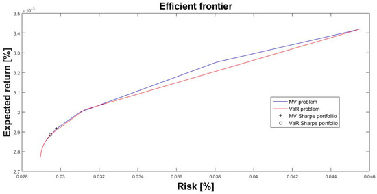
Figure 2.
“Efficient frontiers” of MV (mean-variance) and VaR (bi-level) problems.
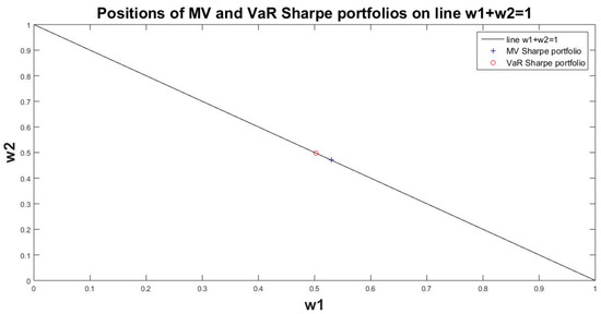
Figure 3.
Positions of portfolios’ MV and VaR on the constraint w1 + w2 = 1.
Both solutions belong to the line , which defines the places of weights of both assets. The bi-level solution gives a bit preference to (asset 5MB), which has less individual risk than (asset 5F4), given by the correlation matrix Σ. Despite that the individual mean return of the first asset is higher, , the bi-level model gives priority to the risk decrease by the value of γ in the upper level optimization, simultaneously with risk minimization on the lower level subproblem.
In Figure 4, the convergence of the bi-level portfolio solutions is illustrated by changing the values of .
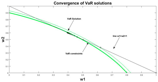
Figure 4.
Convergence of the solutions by changing value of λ.
These solutions are defined at the cross point between the line and the quadratic relation for VaR value:
In Figure 5, the decrease of relation (24), is illustrated by changing the values of to its minimal value. It converges to the lowest curve of VaR constraint (24) and the corresponding minimal value is given on line (24).
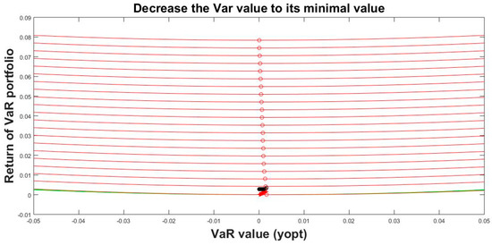
Figure 5.
The convergence of VaR value to its solution from VaR problem (23).
In Figure 6 are presented the values of Sharpe ratios for problems (22) and (23) (the MV and VaR ones), solved by changing the values of .
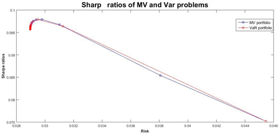
Figure 6.
Sharpe ratios for problems MV and VaR solved by changing the values of .
The graphics are related on the horizontal axis with the corresponding values of the portfolio risks. It is seen that both graphics are very close, but the existing difference results in different values of the maximal Sharpe ratio. Respectively, the contents of the portfolio solutions: and are different. This difference is presented by different places of both solutions on Figure 2 and Figure 3.
6. Conclusions
This work presents a new bi-level model for a portfolio optimization problem. The upper level performs minimization of the VaR portfolio value, which defines the maximal portfolio loss for a given market conditions, estimated by the mean asset returns and Σ. The VaR parameter is regarded as a quantitative measure of the investment sustainability. It defines the risk and the maximum likely loss of the portfolio decision. The VaR parameter is influenced by the confidence level α but by having the levels of practical confidence usage, it takes one predefined value: 90%, 95% and/or 99%. The low level subproblem simultaneously performs minimization of the portfolio risk and maximizes the portfolio return, defined according to the relation of MV model. The comparison between the modified MV model and the bi-level one gives preferences to the bi-level one because it gives a larger set of optimal solutions: the optimal weights of the portfolio assets and the optimal VaR value . A peculiarity of the derived bi-level model is its preference towards risk minimization. The comparison between the portfolio risks and returns gives more safe solutions for the bi-level model because it gives lower level of portfolio risk. The graphical interpretation of the bi-level model shows that the portfolio solutions are the crossing point between the line and the corresponding quadratic curve, formalizing the relation between the VaR parameters and the portfolio weights w.
This bi-level approach can be extended to optimize other forms of probabilistic risks as Conditional VaR, but this can be given in separate research, so as not to complicate the current conclusions.
Author Contributions
Conceptualization, T.S. and K.S.; methodology, M.V.; software, K.S.; validation, T.S., and M.V.; formal analysis, T.S. and K.S.; investigation, K.S.; resources, M.V.; data curation, M.V.; writing—original draft preparation, T.S., K.S.; writing—review and editing, T.S., K.S.; visualization, K.S.; supervision, M.V.; project administration, T.S.; funding acquisition, T.S. All authors have read and agreed to the published version of the manuscript
Funding
This research was funded by Bulgarian National Science fund, grant number ДH12/10, 20.12.2017. The APC was funded by Bulgarian National Science fund.
Conflicts of Interest
The authors declare no conflict of interest.
Notation List
| MV | Mean Variance (portfolio model) |
| VaR | Value at Risk (probabilistic form of formalization of the portfolio risk) |
| CVaR | Conditional VaR (integrated form of evaluation of VaR) |
| CAPM | Capital Asset Pricing Model (the model introduces the meaning of market portfolio) |
| BL | Black-Litterman model (introduces explicitly, in the portfolio problem, quantifications of the expert views about the levels of future asset returns) |
| MAD | Mean Absolute Deviation (particular form if introducing linear relation for the portfolio risk) |
| Bi-level | hierarchical form of interconnected optimization problems |
References
- Sharpe, W. Portfolio Theory and Capital Market; McGraw Hill: London, UK, 1999; 316p. [Google Scholar]
- Markowitz, H. Portfolio selection. J. Financ. 1952, 7, 77–91. Available online: https://www.math.ust.hk/~maykwok/courses/ma362/07F/markowitz_JF.pdf (accessed on 18 February 2021).
- Black, F.; Litterman, R. Asset Allocation: Combining investor views with market equilibrium. J. Fixed Income 1991, 1, 7–18. [Google Scholar] [CrossRef]
- Hoe, L.W.; Hafizah, J.S.; Zaidi, I. An empirical comparison of different risk measures in portfolio optimization. J. Bus. Econ. Horiz. 2010, 1, 39–45. Available online: https://academicpublishingplatforms.com/docs/BEH/Volume1/06_V1_MALAYSIA_BEH_Lam%20Weng_Hafizah_d.pdf (accessed on 18 February 2021).
- Stoilov, T.; Stoilova, K.; Vladimirov, M. Analytical Overview and Applications of Modified Black-Litterman Model for Portfolio Optimization. J. Cybern. Inf. Technol. 2020, 20, 30–49. Available online: http://www.cit.iit.bas.bg/CIT-2020/v-20-2/10341-Volume20_Issue_2-03_paper.pdf (accessed on 18 February 2021). [CrossRef]
- Dempe, S. Bi-level Optimization: Theory, Algorithms, Applications and a Bibliography. In Bi-level Optimization; Dempe, S., Zemkoho, A., Eds.; Springer Optimization and Its Applications (SOIA): Cham, Switzerland, 2020; Volume 161, pp. 581–672. Available online: https://link.springer.com/chapter/10.1007/978-3-030-52119-6_20#citeaspringer (accessed on 18 February 2021)ISBN 978-3-030-52118-9. [CrossRef]
- Stoilov, T.; Stoilova, K.; Vladimirov, M. Modeling and assessment of financial investments by portfolio optimization on stock exchange. In Advances in High Performance Computing, Studies in Computational Intelligence; Dimov, I., Fidanova, S., Eds.; Springer: Heidelberg, Germany, 2020; pp. 340–356. [Google Scholar] [CrossRef]
- Bonami, P.; Lejeune, M.A. An exact solution approach for portfolio optimization problems under stochastic and integer constraints. J. Oper. Res. 2009, 57, 650–670. Available online: http://www.optimization-online.org/DB_FILE/2007/02/1580.pdf (accessed on 18 February 2021). [CrossRef]
- Chen, Z.; Zhuang, X.; Liu, J. A Sustainability-Oriented Enhanced Indexation Model with Regime Switching and Cardinality Constraint. Sustainability 2019, 11, 4055. [Google Scholar] [CrossRef]
- Krokhmal, P.; Palmquist, J.; Uryasev, S. Portfolio optimization with conditional value-at-risk objective and constraints. J. Risk 2002, 4, 11–27. Available online: http://citeseerx.ist.psu.edu/viewdoc/download?doi=10.1.1.4.1197&rep=rep1&type=pdf (accessed on 18 February 2021). [CrossRef]
- Stoilov, T.; Stoilova, K.; Vladimirov, M. Saving Time in Portfolio Optimization on Financial Markets. Application of Decision Science in Business and Management. Available online: https://www.intechopen.com/online-first/saving-time-in-portfolio-optimization-on-financial-markets (accessed on 18 February 2021).
- Mencarelli, L.; D’Ambrosio, C. Complex portfolio selection via convex mixed-integer quadratic programming: A survey. Int. Trans. Oper. Res. 2002, 26, 389–414. Available online: https://onlinelibrary.wiley.com/doi/abs/10.1111/itor.12541 (accessed on 18 February 2021). [CrossRef]
- Park, S.; Lee, E.R.; Lee, S.; Kim, G. Dantzig Type Optimization Method with Applications to Portfolio Selection. Sustainability 2019, 11, 3216. [Google Scholar] [CrossRef]
- Oprisor, R.; Kwon, R. Multi-Period Portfolio Optimization with Investor Views under Regime Switching. J. Risk Financ. Manag. 2021, 14, 3. Available online: https://www.mdpi.com/1911-8074/14/1/3/pdf (accessed on 18 February 2021). [CrossRef]
- Khan, K.I.; Naqvi, S.M.W.A.; Ghafoor, M.M.; Akash, R.S.I. Sustainable Portfolio Optimization with Higher-Order Moments of Risk. Sustainability 2020, 12, 2006. [Google Scholar] [CrossRef]
- Kuester, K.; Mittnik, S.; Paolella, M.S. Value-at-Risk Prediction: A Comparison of Alternative Strategies. J. Financ. Econom. 2006, 4, 53–89. Available online: https://pdfs.semanticscholar.org/d5c1/05ffa2508f63a0c1f2123b77189a35e5dcab.pdf (accessed on 18 February 2021). [CrossRef]
- El-Wahed Khalifa, H.A.; Alharbi, M.G.; Kumar, P. A new approach for the optimization of portfolio selection problem in fuzzy environment. Adv. Math. Sci. J. 2020, 9, 7171–7190. [Google Scholar] [CrossRef]
- Deng, X.T.; Li, Z.F.; Wang, S.Y. A minimax portfolio selection strategy with equilibrium. Eur. J. Oper. Res. 2005, 166, 278–292. [Google Scholar] [CrossRef]
- Polak, G.; Rogers, D.F.; Sweeney, D.J. Risk management strategies via minimax portfolio optimization. Eur. J. Oper. Res. 2010, 207, 409–419. Available online: https://www.sciencedirect.com/science/article/abs/pii/S0377221710003449 (accessed on 18 February 2021). [CrossRef]
- Sharma, A.; Mehra, A. Portfolio selection with a minimax measure in safety constraint. J. Math. Program. Oper. Res. 2013, 62, 1473–1500. [Google Scholar] [CrossRef]
- Zaimović, A.; Sikalo, M.; Arnaut-Berilo, A. Efficiency of the minmax portfolio on the European capital market—Can we beat the market. Pressacademia 2017, 6, 78–87. Available online: https://dergipark.org.tr/en/download/article-file/379417 (accessed on 18 February 2021).
- Kobayashi, K.; Takano, Y.; Nakata, K. Bilevel Cutting-plane Algorithm for Solving Cardinality-constrained Mean-CVaR Portfolio Optimization Problems. Comput. Sci. Math. Optim. Control 2020. Available online: https://arxiv.org/pdf/2005.12797.pdf (accessed on 18 February 2021).
- Benita, F.; López-Ramos, F.; Nasini, S. A bi-level programming approach for global investment strategies with financial intermediation. Eur. J. Oper. Res. 2019, 274, 375–390. Available online: https://www.sciencedirect.com/science/article/abs/pii/S0377221718308609 (accessed on 18 February 2021). [CrossRef]
- Kalashnikov, V.; Kalashnykova, N.; Leal-Coronado, M. Solution of the portfolio optimization model as a bi-level programming problem. Вісник Черкаськoгo університету 2017, 54–65. Available online: http://econom-ejournal.cdu.edu.ua/article/view/1953/2026 (accessed on 18 February 2021).
- Jing, K.; Xu, F.; Li, X. A bi-level programming framework for identifying optimal parameters in portfolio selection. Int. Trans. Oper. Res. 2020, 41. Available online: https://onlinelibrary.wiley.com/doi/epdf/10.1111/itor.12856 (accessed on 18 February 2021). [CrossRef]
- Konno, H.; Yamazaki, H. Mean-Absolute Deviation Portfolio Optimization Model and Its Applications to Tokyo Stock Market. Manag. Sci. 1991, 37, 519–531. [Google Scholar] [CrossRef]
- Bower, B.; Wentz, P. Portfolio Optimization: MAD vs. Markowitz. Rose-Hulman Undergrad. Math. J. 2005, 6. Available online: https://scholar.rose-hulman.edu/rhumj/vol6/iss2/3 (accessed on 18 February 2021).
- Dowd, K. Measuring Market Risk, 2nd ed.; John Wiley & Sons, Inc.: Hoboken, NJ, USA,, 2005; 390p, Available online: https://www.academia.edu/28033721/Measuring_Market_Risk_Second_Edition (accessed on 18 February 2021).
- Chen, J.M. On Exactitude in Financial Regulation: Value-at-Risk, Expected Shortfall, and Expectiles. J. Risks 2018, 6, 61. Available online: https://www.mdpi.com/2227-9091/6/2/61 (accessed on 18 February 2021). [CrossRef]
- Li, Z.; Li, X.; Hui, Y.; Wong, W.K. Maslow Portfolio Selection for Individuals with Low Financial Sustainability. Sustainability 2018, 10, 1128. [Google Scholar] [CrossRef]
- Sukono, S.P.; Talib bin Bon, A.; Supian, S. Modeling of Mean-VaR Portfolio optimization by Risk Tolerance When the Utility Function is Quadratic. 2017, p. 020035. Available online: https://aip.scitation.org/doi/pdf/10.1063/1.4979451 (accessed on 18 February 2021).
- Larsen, N.; Mausser, H.; Uryasev, S. Algorithms for Optimization of Value-at-Risk. In Financial Engineering, E-Commerce and Supply Chain. Applied Optimization; Pardalos, P.M., Tsitsiringos, V.K., Eds.; Springer: Boston, MA, USA, 2002; Volume 70, Available online: http://www.pacca.info/public/files/docs/public/finance/Active%20Risk%20Management/Uryasev%20-%20Algorithms%20Optimization%20VaR.pdf (accessed on 18 February 2021).
- Wang, D.; Chen, Y.; Wang, H.; Huang, M. Formulation of the Non-Parametric Value at Risk Portfolio Selection Problem Considering Symmetry. Symmetry 2020, 12, 1639. Available online: https://www.mdpi.com/2073-8994/12/10/1639 (accessed on 18 February 2021). [CrossRef]
- Lwin, K.T.; Qu, R.; MacCarthy, B.L. Mean-VaR portfolio optimization: A nonparametric approach. Eur. J. Oper. Res. 2017, 260. Available online: https://www.researchgate.net/profile/Khin_Lwin4/publication/312131359_Mean-VaR_Portfolio_Optimization_A_Nonparametric_Approach/links/59f50366458515547c21cdec/Mean-VaR-Portfolio-Optimization-A-Nonparametric-Approach.pdf (accessed on 18 February 2021). [CrossRef]
- Pelegrin da Silvaa, L.; Alema, D.; Leonel de Carvalhoa, F. Portfolio optimization using Mean Absolute Deviation (MAD) and Conditional Value-at-Risk (CVaR). Production 2017, 27. Available online: http://www.scielo.br/scielo.php?script=sci_arttext&pid=S0103-65132017000100302 (accessed on 18 February 2021). [CrossRef]
- Acerbi, C.; Tasche, D. On the coherence of expected shortfall. J. Bank. Available online: https://arxiv.org/abs/cond-mat/0104295 (accessed on 18 February 2021). [CrossRef]


Publisher’s Note: MDPI stays neutral with regard to jurisdictional claims in published maps and institutional affiliations. |
© 2021 by the authors. Licensee MDPI, Basel, Switzerland. This article is an open access article distributed under the terms and conditions of the Creative Commons Attribution (CC BY) license (http://creativecommons.org/licenses/by/4.0/).