Article

Utility of Remotely Sensed Evapotranspiration Products to Assess an Improved Model Structure

1
School of Environmental Engineering, University of Seoul, 163 Seoulsiripdae-ro, Dongdaemun-gu, Seoul 02504, Korea
2
Earth System Science Interdisciplinary Center, University of Maryland, College Park, MD 20740, USA
3
Department of Engineering Systems and Environment, University of Virginia, Charlottesville, VA 22904, USA
4
School of Data Science, University of Virginia, Charlottesville, VA 22904, USA
5
USDA-ARS, Hydrology and Remote Sensing Laboratory, Beltsville, MD 20705, USA
6
Joint Global Change Research Institute, Pacific Northwest National Laboratory and University of Maryland, College Park, MD 20740, USA
7
Department of Environmental Science & Technology, University of Maryland, College Park, MD 20742, USA
*
Author to whom correspondence should be addressed.
Sustainability 2021, 13(4), 2375; https://doi.org/10.3390/su13042375
Submission received: 1 February 2021 / Revised: 17 February 2021 / Accepted: 18 February 2021 / Published: 23 February 2021

Abstract

:
There is a certain level of predictive uncertainty when hydrologic models are applied for operational purposes. Whether structural improvements address uncertainty has not well been evaluated due to the lack of observational data. This study investigated the utility of remotely sensed evapotranspiration (RS-ET) products to quantitatively represent improvements in model predictions owing to structural improvements. Two versions of the Soil and Water Assessment Tool (SWAT), representative of original and improved versions, were calibrated against streamflow and RS-ET. The latter version contains a new soil moisture module, referred to as RSWAT. We compared outputs from these two versions with the best performance metrics (Kling–Gupta Efficiency [KGE], Nash-Sutcliffe Efficiency [NSE] and Percent-bias [P-bias]). Comparisons were conducted at two spatial scales by partitioning the RS-ET into two scales, while streamflow comparisons were only conducted at one scale. At the watershed level, SWAT and RSWAT produced similar metrics for daily streamflow (NSE of 0.29 and 0.37, P-bias of 1.7 and 15.9, and KGE of 0.47 and 0.49, respectively) and ET (KGE of 0.48 and 0.52, respectively). At the subwatershed level, the KGE of RSWAT (0.53) for daily ET was greater than that of SWAT (0.47). These findings demonstrated that RS-ET has the potential to increase prediction accuracy from model structural improvements and highlighted the utility of remotely sensed data in hydrologic modeling.

1. Introduction

Water resource management is important for resource allocation in agricultural and mixed land-use watersheds, to accommodate for the rising water demand as a result of population increase. An improved understanding of water resource dynamics aids the development of effective adaptation strategies [1]. Hydrologic models are often used as a means to design and manage water resource systems [2,3,4]. Although the use of these models for operational purposes may provide practical solutions, there is a need for continuous effort to reduce uncertainty involved in operational applications of hydrologic models [5,6].
Hydrologic models include a large number of parameters that represent physical and biogeochemical processes with high spatio-temporal heterogeneity within landscapes [7]. Most parameters cannot be measured via in-situ observations; calibration of these parameters produces the best goodness-of-fit between simulated and monitored fluxes at the watershed outlet [8]. This typical calibration approach may not replicate physical and biogeochemical fluxes within watersheds, resulting in less reliable simulations [9,10]. Improvements in calibration may involve monitoring multiple fluxes at the outlet (e.g., streamflow and nutrient loads), and including additional soft data (e.g., intra-watershed measurements, expert knowledge, remotely sensed data, and local statistics) [11,12]. For example, soft data use in hydrological modeling may involve limiting parameter spaces with an additional constraint [13], semi-spatially explicit characterization of inundation parameters [14], use of local knowledge to constrain nutrient concentrations in different pathways [10], modification of the denitrification parameter based on local knowledge to better represent landscape biogeochemistry [15], and constraints on parameter spaces based on the remotely sensed leaf area index [16]. Furthermore, model calibration against satellite-driven vegetation data led to advanced prediction of vegetation growth and recovery from fire [17]. The addition of root zone soil moisture to model calibration was proven to reduce parameter sampling spaces as well as uncertainty [18].
In addition to improved parameterization, model structure refinements to better describe hydrological processes have been suggested to reduce model uncertainty [5,19]. Cho et al. [20] modified a bacterial module to improve the prediction of fecal contamination. The development of a physically based soil-temperature module enabled the improved representation of soil temperature conditions [21]. A modified hydrologic model with a discretized aquifer representation produced better characterization of baseflow in a lowland catchment [22]. Water volume storage within depressional wetlands was also well captured by improved representation of vertical and horizontal water movement within a hydrologic model [23]. The addition of a new external module in a hydrologic model that simulates the hydrological connection between riparian wetlands and adjacent streams has enabled the quantification of impacts from riparian wetlands on sediment loads and streamflow [24]. A hydrologic model coupled with a module that represents the fate and transport of carbon was found to effectively capture dissolved and particulate organic carbon loads [25]. A recent study further improved the carbon cycling within in-streams to better predict carbon fluxes [26]. A model coupled with a water temperature module showed improved predictions of water quality variables affected by water temperature [27]. These model improvements have been quantitatively assessed with additional observations to monitor specific refined processes.
It is often challenging to depict clear differences between existing and modified model structures due to a lack of data. When model evaluation was largely dependent on streamflow data, there was limited ability to distinguish the advantages of modified model structures relative to the original structure [28,29]. For example, Evenson et al. [28] reported that the performance metric (Nash-Sutcliffe Efficiency (NSE) and a ratio of the root mean square error to the standard deviation (RSR)) for streamflow prediction was almost similar between an existing model (0.67 and 0.58) and the improved model (0.66 and 0.58). Establishing in-situ monitoring instruments may address this issue; however, these are often expensive and labor-intensive [30]. Alternatively, remotely sensed data are capable of characterizing and monitoring land surface information across landscapes over long periods of time, and the data collected may support hydrologic modeling by providing additional constraints [31,32]. However, few studies attempted to use remotely sensed data for demonstrating the contribution of model structure improvements.
This study capitalizes on remotely sensed data to assess an improved soil moisture module within a hydrologic model; the Soil and Water Assessment Tool (SWAT). Qi et al. [33] incorporated a physically-based soil moisture module (i.e., the Richard equation-based module) into SWAT, producing the RSWAT. Qi et al. [29] compared SWAT and RSWAT to test the efficacy with which RSWAT replicates the partitioning of water into surface runoff and infiltration. They found that SWAT and RSWAT were similar in prediction capacity, likely due to the limitations of data sources that constrained model outputs [29]. This study employs remotely sensed evapotranspiration (RS-ET) products as an additional constraint to discern differences between SWAT and RSWAT. Evapotranspiration (ET) is the sum of evaporation and transpiration, and a crucial component in water and energy exchange between atmospheric and terrestrial systems [34]. ET may be an indicator for accurately representing water partitioning on the land surface [35]. To quantitatively assess model performance, we adopted the Kling–Gupta Efficiency (KGE) measure for daily streamflow and ET as an objective function (see Section 2.5). Two metrics (NSE and Percent-bias (P-bias)) were used as additional objective functions for daily streamflow.
First, SWAT and RSWAT were calibrated against streamflow and watershed level RS-ET; their outputs were subsequently compared at the watershed level. Then, the ET outputs from SWAT and RSWAT were compared at a finer spatial level using a subwatershed level RS-ET. These comparisons were used to test the ability of RS-ET to further constrain outputs from different versions of SWAT, and improve the ability to discern performance differences resulting from different model structures.

2. Materials and Methods

2.1. Study Area

This study used the drainage area of Tuckahoe Creek, as defined by the United States Geological Survey (USGS) gauge station located near Ruthsburg, Maryland (USGS#01491500); this is referred to as the Tuckahoe Creek Watershed (TCW, 220 km2). The TCW is located within the upper region of the Choptank River watershed (CRW) within the Delmarva Peninsula (Figure 1a). This region is categorized as a temperate, humid climate zone receiving an annual average precipitation of 1200 mm [36]. Seasonal precipitation is evenly distributed throughout the year, while ET is low in the wet season (December to May) and high in the dry season (June to November) [37]. Land use in the TCW is dominated by croplands (54%) that cultivate corn, soybean, and winter wheat (Figure 1b). The use of irrigated water for corn and soybean has been increasing in this region, contributing to changes in ET dynamics during the dry season [38]. The remaining area in the TCW is comprised of forest (33%), pasture (8%), urban (4%), and water bodies (1%). Well-drained soils (hydrologic soil groups—A and B) account for a slightly greater portion of the watershed (56%) relative to poorly drained soils (C and D, 44%).

2.2. Description of SWAT

SWAT is a semi-distributed, watershed-scale water quality model capable of monitoring the impacts of environmental and anthropogenic changes on physical processes in an agricultural watershed [40]. The model partitions a watershed into subwatersheds, and further into hydrologic response units (HRUs); the latter are a unique combination of land use, soil, and slope within a subwatershed. All hydrological outputs were computed for individual HRUs. The partitioning between surface runoff and infiltration may be calculated using the Soil Conservation Service curve number (CN) procedure or the Green and Ampt infiltration method in SWAT. The CN method was used in this study as it is prevalent in the literature.
The CN method calculates the daily surface runoff ( Q s u r f , mm·d−1) using daily rainfall depth ( R d a y , mm·d−1), and the retention parameter ( S , mm·d−1). The latter is determined by the C N and differs based on the land use, soil permeability, and antecedent soil water conditions:
Q s u r f = ( R d a y 0.2 · S ) 2 ( R d a y + 0.8 · S )
S = 25.4 · ( 1000 C N 10 )
The retention parameter by soil profile water content is expressed as:
S = S m a x · ( 1 S W [ S W + exp ( w 1 w 2 · S W ) ] )
where S m a x is the maximum value of retention on a given day (mm·d−1); SW is the soil water content of the entire profile excluding the amount of water held in the profile at wilting point; and w 1 and w 2 are shape coefficients.
Infiltrated water affects the soil water dynamics in SWAT. The daily soil water content in each layer was determined as follows:
Δ S W i = Q p , i l Q p , i Q l , i E e , i E t , i
where Δ S W i is the change in soil water content (mm) at the i th soil layer; Q p , i l is the percolation from the upper layer (mm); Q p , i is the percolation out of the current soil layer (mm); Q l , i is the lateral flow generated from the current soil layer (mm); and E e , i and E t , i are the evaporation and transpiration drawn from the current soil layer (mm), respectively. The percolation ( Q p , i ) for the ith layer is expressed as:
Q p , i = ( S W i F C i ) [ 1 exp ( 24 K s a t , i S A T i F C i ) ]
where F C i is the soil water content at field capacity (mm); K s a t , i is the saturated hydraulic conductivity (mm·h−1); and S A T i is the amount of water required for the complete saturation (mm) of the i th layer. Percolation from the bottom of the soil profile enters groundwater, and lateral flow was modeled using a kinematic storage routing method based on the slope, slope length, and saturated conductivity. SWAT has three methods for reference ET calculations [40]: the Penman–Monteith, Priestley–Taylor, and Hargreaves methods. We used the Penman–Monteith method to compute E T r as follows:
E T r = Δ · ( H n e t G ) + ρ a i r · c p · [ e z 0 e z ] / r a Δ + γ · ( 1 + r c / r a )
where E T r is the maximum transpiration rate (mm·d−1); Δ is the slope of the saturation vapor pressure–temperature curve (kPa·°C−1); H n e t is the net radiation (MJ·m−2 d−1); G is the heat flux density to the ground (MJ·m−2 d−1); ρ a i r is the density of air (kg·m−3); c p is the specific heat at constant pressure (MJ·kg−1 °C−1); e z 0 is the saturation vapor pressure of air at height z (kPa); e z is the water vapor pressure of air at height z (kPa); γ is the psychrometric constant (kPa·°C−1); r c is the plant canopy resistance (s·m−1); and r a is the diffusion resistance of the air layer (aerodynamic resistance) (s·m−1). Further details are available in Neitsch et al. [40].

2.3. RSWAT

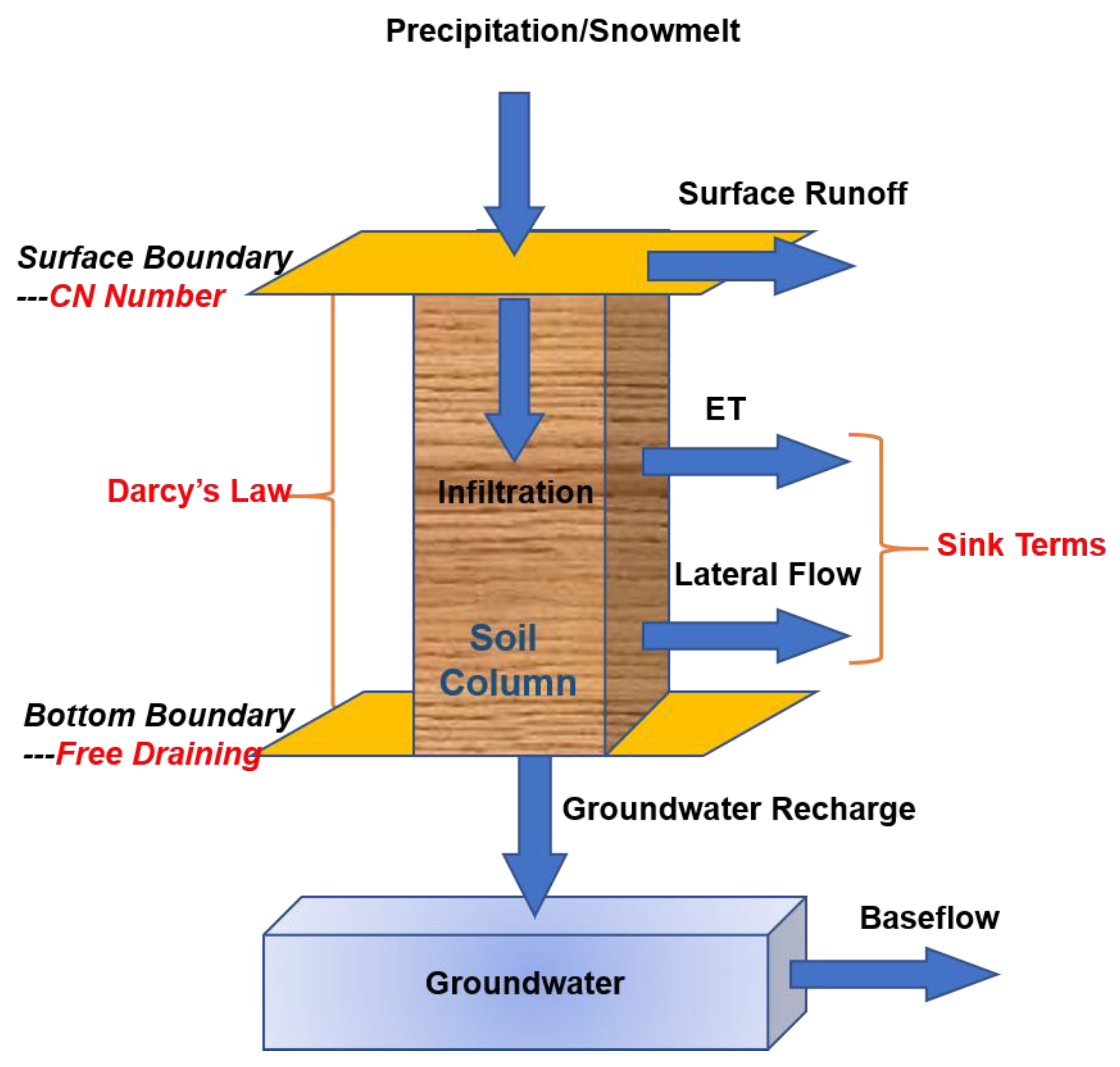
Qi et al. [33] generated a new version of SWAT by incorporating a modified Richards equation into the model to physically represent soil water content and moisture movement (Figure 2). The Richards equation-based soil moisture module was tested against field measurements and compared with the original soil moisture module at 10 stations within the CRW. The results show that the Richards equation-based module outperformed the original module in terms of simulations of daily soil moisture based on the improved R-squared and reduced biases [33]. Here, we briefly introduce the Richards-equation-based soil moisture module; detailed information on model development and evaluation is provided in Qi et al. [33].
The modified Richards equation incorporated in RSWAT is as follows:
θ t = z [ k ( ( h h e ) z ) ] Q
where θ is the volumetric soil water content (mm3·mm−3); t is time (s); z is the depth below the soil surface (mm; positive downward); k is the hydraulic conductivity (mm·s−1); h is the soil matric potential (mm); Q is the soil water sink term (mm·mm−1 s−1); and h e is the equilibrium soil matric potential (mm). Equation (7) was discretized into a set of tridiagonal equations solved using the method of Patankar [41]. Infiltration was determined using the surface boundary condition from the CN method, and assuming free-draining conditions for the bottom boundary condition. Evaporation, transpiration, and lateral flow are the sink terms in Equation (7) that were calculated using their corresponding SWAT functions. Instantaneous hydraulic conductivity was estimated using the Community Land Model [42], while saturated conductivity was measured and provided in each HRU based on the US Department of Agriculture (USDA) Natural Resources Conservation Service (NRCS) Soil Survey Geographic Database (SSURGO). According to Clapp and Hornberger [43] and Cosby et al. [44], soil matric potential is a function of water content and hydraulic conductivity. The equilibrium soil matric potential considers the impact of fluctuations in the water table, and was determined based on the method of Zeng and Decker [45].

2.4. SWAT Input Data and Model Constraints

Meteorological and geospatial data were used to run the SWAT (Table 1). SWAT input data consisted of the National Aeronautics and Space Administration (NASA) North American Land Data Assimilation System 2 (NLDAS2) forcing data, including hourly precipitation, temperature, solar radiation, relative humidity, and wind speed. The NLDAS2 data is generated by multiple observations that provide continental-scale data at a spatial resolution of 1/8° [46]. A light detection and ranging (LiDAR)-based digital elevation model of the USDA-Agricultural Research Service (Beltsville, MD, USA) was used to establish the topographic characteristics and divide modeling units. A soil map was downloaded from the SSURGO database, while the land use map utilized in this study was developed by Lee et al. [47]. This land use map characterized farmland configurations and annually cultivated crops using multi-year cropland data layers (CDLs). The spatial distribution of other types of land-use were identified using multiple geospatial datasets (Table 1); Lee et al. [47] provides further details.
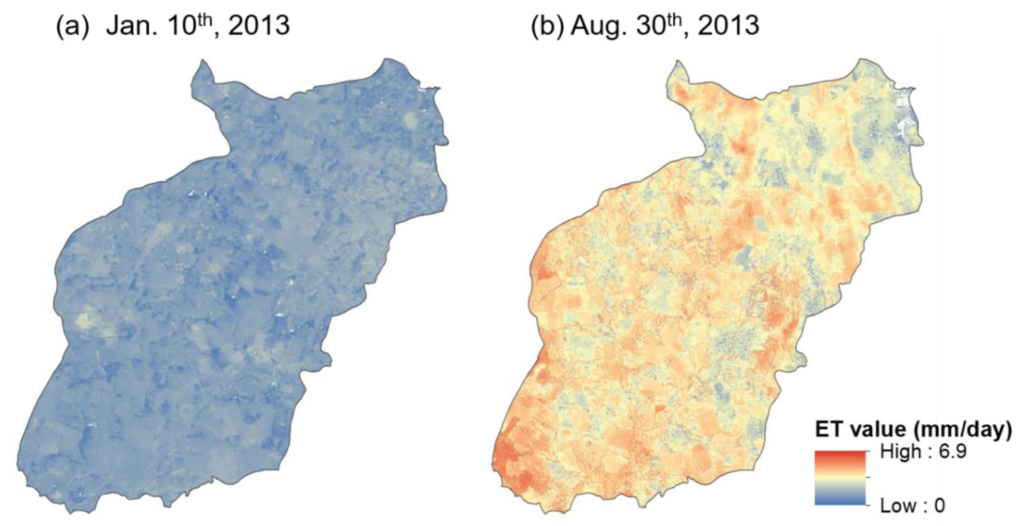
Streamflow and RS-ET were used as model constraints; daily streamflow records from 2010 to 2014 were obtained from USGS gauge station #01491500 (Figure 1a). RS-ET data were developed by the regional Atmosphere-Land Exchange Inverse (ALEXI) model [49,50] and the associated flux spatial–temporal disaggregation scheme (DisALEXI, Anderson et al., 2004). The 30 m daily RS-ET data from ALEXI/DisALEXI in the study area has been previously validated against in-situ eddy covariance flux tower measurements, with an average relative error of 10% [48]. Figure 3 presents examples of 30 m daily RS-ET data for the TCW; this data spans from January 2010 to December 2014 and was utilized as an additional model constraint. The watershed level average of the RS-ET was calculated for model calibration.

2.5. Model Calibration

SWAT and RSWAT were calibrated at a daily time step over five years (2010–2014), as streamflow and RS-ET were available during this period. A warm-up period of two years (2008–2009) was used for the calibration. The simulation periods were not split into calibration and validation periods due to the short-term observations. The model simulation guidelines outlined by Arnold et al. [51] recommends the inclusion of different climate conditions (e.g., dry and wet) during the calibration period to identify optimal parameter values for sites of interest. In addition, a study comparing performances between two models often only considered a calibration period [28]. As RSWAT and SWAT were tested at the same study site, we used a five-year calibration period to identify the best parameter values for SWAT and RSWAT. Previous SWAT modeling studies conducted in the study area have demonstrated the sensitivity of streamflow and water quality parameters [36,52]. Based on these studies, we established 13 parameters to calibrate SWAT and RSWAT against streamflow and RS-ET (Table 2). We prepared 1000 parameter sets using the Latin hypercube sampling (LHS) method that efficiently identifies the optimal parameter set [53]; thus, the parameter set producing the best model performance measures was identified.
The KGE was used to simulate streamflow and ET against corresponding observations. KGE diagnostically decomposes the NSE and mean squared error (MSE) to provide a combined measure of the relative importance of correlation, bias, and variability for hydrological modeling [54]. KGE values range from −∞ to 1, where values closer to 1 indicate a stronger model performance:
K G E = 1 ( r 1 ) 2 ( σ r / σ o 1 ) 2 ( μ r / μ o 1 ) 2
where r indicates the Pearson product-moment correlation coefficient; σ s / σ o and μ s / μ o indicate the variability ratio and bias between simulations and observations, respectively; σ and μ indicate the standard deviation and mean of the variables, respectively; and the subscripts, s and o , indicate the simulations and observations, respectively. We additionally used NSE and P-bias as the metrics for daily streamflow. NSE is an indicator of how well simulated and observed values fit the 1:1 line and the range of NSE is from −∞ to 1 (one indicates a perfect fit) [55]. P-bias indicates a general tendency of model over-(or under-) prediction relative to observations, and positive and negative values refer to model underestimation and overestimation, respectively [55]. Lower and greater values refer to increased and decreased accuracy, respectively. The two metrics have been frequently adopted to assess daily performance measures [52,56] and they are calculated as follows:
N S E = 1 [ i = 1 n ( O i S i ) 2 i = 1 n ( O i O ¯ ) 2 ]
P - b i a s = [ i = 1 n ( O i S i ) × 100 i = 1 n O i ]
where O i are observed and S i are simulated data; O ¯ are observed mean values; and n equals the number of observations. The “hydroGOF” package of the R program [57] was used to calculate KGE, NSE, and P-bias.

2.6. Comparing the Prediction Capacity of SWAT and RSWAT

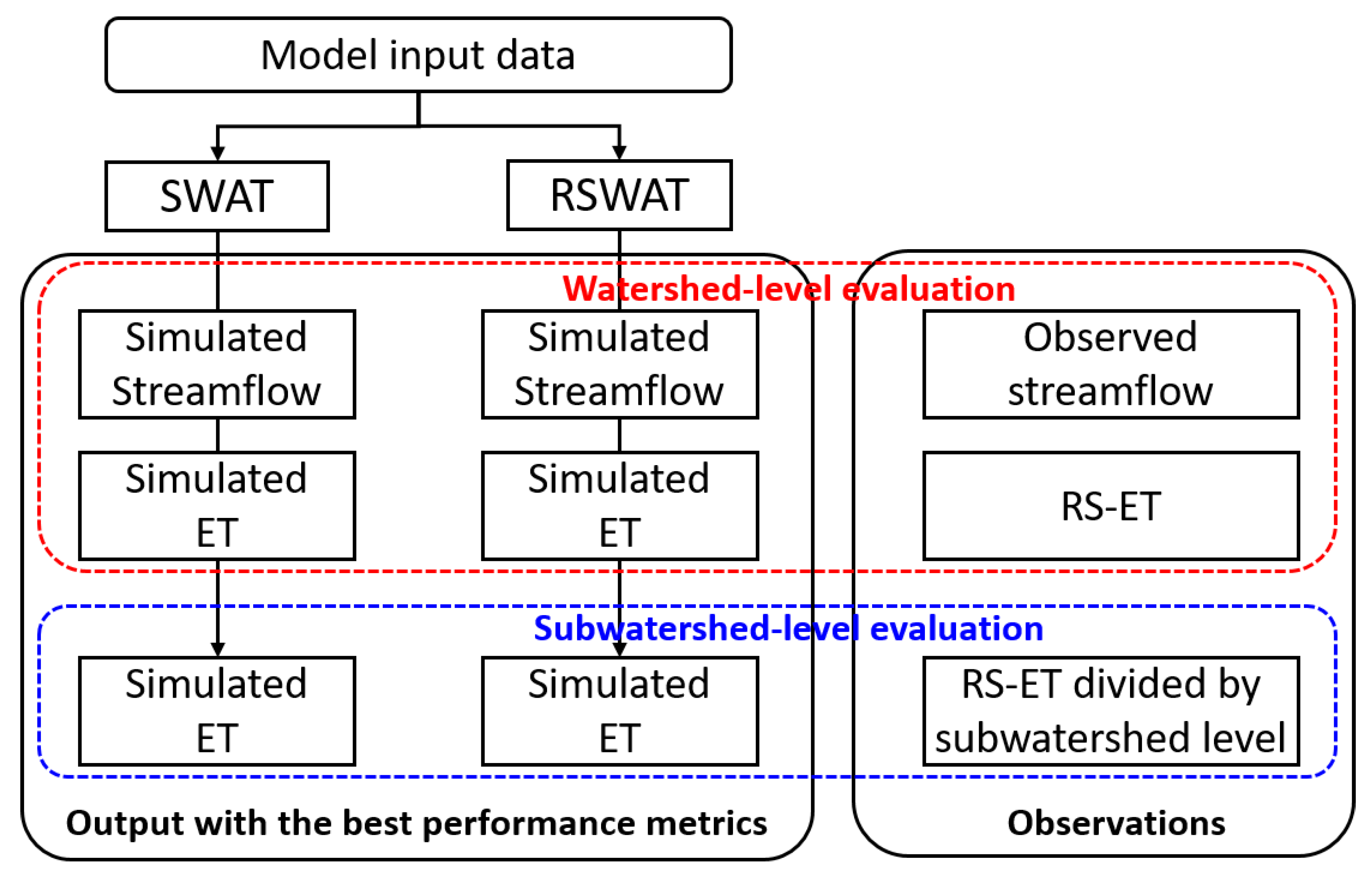
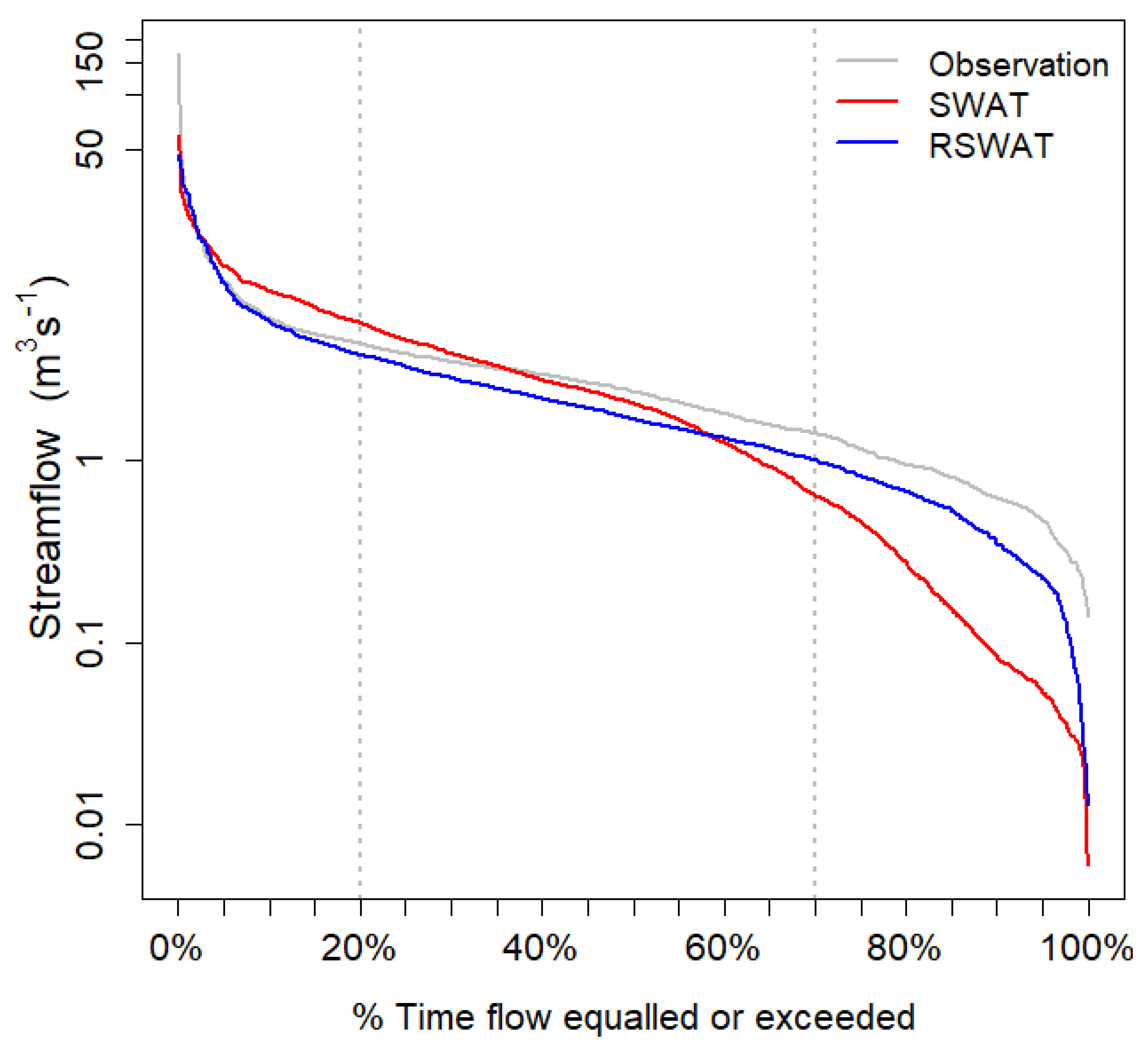
To demonstrate how representative the modified model structure (i.e., RSWAT) was for hydrologic variables, we conducted evaluations at two spatial levels (Figure 4). Simulated streamflow and watershed level ET simulations from SWAT and RSWAT were first examined using observed streamflow and RS-ET, respectively. A flow duration curve (FDC) was plotted using daily streamflow from SWAT and RSWAT to examine how the two models replicate streamflow during high and low-flow periods compared to observations. Then, subwatershed-level assessments were conducted by comparing the subwatershed-level ET and the corresponding RS-ET divided by the subwatershed boundary. There are 19 subwatersheds spanning from 0.09 to 32 km2 in the TCW. The subwatershed boundary was delineated using the ArcSWAT interface for SWAT with an input DEM [58]. Subwatershed-level model outputs were directly obtained from the SWAT and RSWAT results, as they represent the best performance metrics at the watershed level. Once the daily subwatershed-level average of RS-ET was determined, the KGE values for individual subwatersheds over the simulation period were calculated for SWAT and RSWAT. Evaluation of streamflow predictions at the subwatershed-level was not conducted due to the absence of subwatershed-level streamflow observations.

3. Results and Discussion

3.1. Streamflow and ET Predictions at the Watershed Level

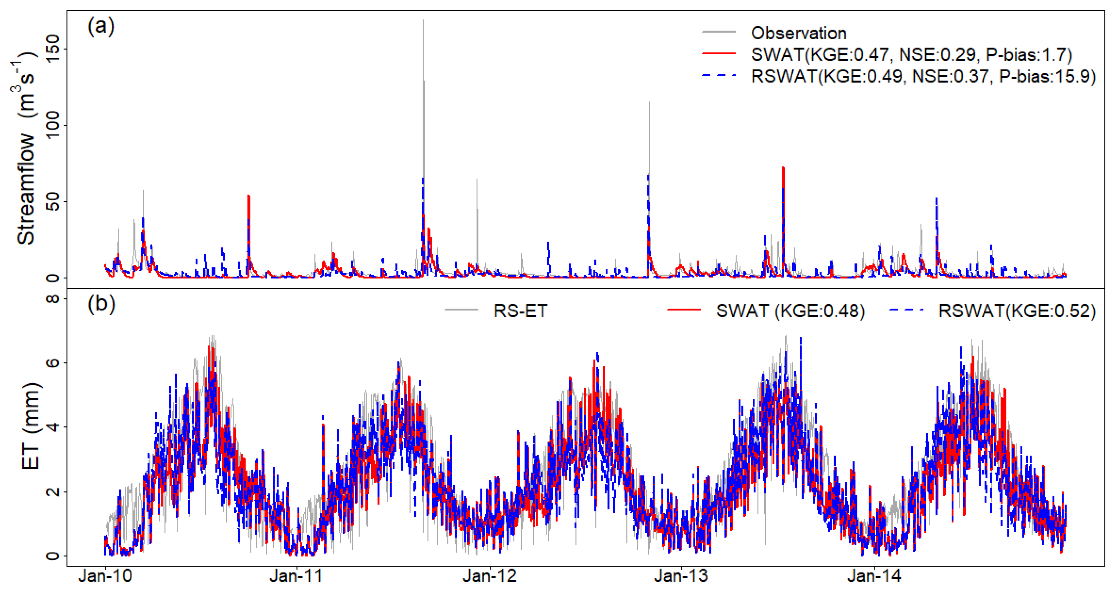
Figure 5 presents the relationship between simulated streamflow and ET from SWAT and RSWAT and the observed streamflow and watershed-level RS-ET. SWAT produced KGE of 0.47, NSE of 0.29, and P-bias of 1.7% for daily streamflow and KGE of 0.48 for daily ET. RSWAT had slightly higher metrics with KGE of 0.49 and NSE of 0.37 for daily streamflow and KGE of 0.52 for daily ET while P-bias was 15.9% greater than SWAT. Overall, SWAT and RSWAT showed similar metrics regarding that KGE values were similar between two models, and NSE and P-bias of SWAT indicated lower and greater accuracy than RSWAT, respectively.
Both models replicated the observations reasonably well. NSE and P-bias for daily streamflow were acceptable when NSE > 0.2 and P-bias ≤ ±25%, respectively [52,56]. SWAT and RSWAT satisfied those criteria for streamflow. Regarding KGE values, a previous study defined KGE > 0.5 as an acceptable performance for monthly streamflow [59]. Our streamflow results were slightly lower than KGE of 0.5. Daily simulations are evaluated using relaxed criteria compared to longer time scale (e.g., monthly and annual) outputs since daily outputs depict detailed extreme values [51]. Therefore, our KGE values for daily streamflow seemed to be within an acceptable range. The KGE values for daily ET were greater than one previous study (i.e., 0.26) [60] while being lower than another previous study (i.e., 0.5–0.9) [61]. Less accurate results are likely due to the omission of plant parameters that account for a substantial portion of ET [61], and the exclusion of the impacts of irrigation. A study by [62] showed model parameterization of forest, resulting in more accurate ET predictions relative to default parameters. For croplands, similar findings were observed in a previous study [63]. Approximately 87% of the study watershed is covered by either crops or forest and therefore non-adjusting plant parameters may be a contributor of low accuracy. However, ET values from the two models reflected strong seasonality (e.g., high ET in summer seasons and low ET in winter seasons) in ET in this region [37] and were relatively well matched with RS-ET.
Peak streamflow was not well captured by SWAT and RSWAT, largely due to inherent model limitations. The CN method used in SWAT does not consider rainfall intensity and duration in partitioning surface runoff and infiltration; as such, simulated peak flows tend to be underestimated [64]. A localized precipitation not observed at weather stations often caused model underestimation of peak streamflow in this region [36]. In addition, a semi-distributed SWAT structure oversimplifies water routing at the subwatershed level, producing inaccurate peak flow predictions [52]. This model error may also be due to the climate input data, NLDAS2; Qi et al. [65] compared SWAT simulations with different climate data finding that SWAT results driven by NLDAS2 climate input data underestimated streamflow due to higher daily solar radiation, leading to overestimations of ET.
A comparison between SWAT and RSWAT outputs using the FDC showed that the latter output provided good agreement with observations. This was particularly the case during low-streamflow conditions (i.e., flow intervals that exceed the greatest fraction of time [>80%], Figure 6). This may be partially due to the use of a simplified soil moisture conceptual model in SWAT, such as a bucket [40]. Shahrban et al. [66] also found that a hydrologic model using a bucket concept for soil moisture poorly simulated low-flow conditions relative to a model that used a continuous distribution of soil moisture according to vertical depth. Based on this FDC result, we postulate that RSWAT may have a greater capacity to replicate water partitioning processes than SWAT. In this region, low flows correspond to baseflow conditions, and the amount of baseflow is determined from water partitioning processes within upstream areas [67]. Another possible reason for this low-flow discrepancy between SWAT and RSWAT is to simultaneously constrain model parameters using streamflow and RS-ET. Tobin and Bennett [68] found that the inclusion of ET as an additional constraint enabled the accurate capturing of actual flow patterns. Multiple constraints were known to improve model ability to predict hydrologic variables [59]. It seemed that an original SWAT received less benefits of multiple constraints owing to limited model structure. However, the greater accuracy of baseflow patterns in RSWAT may be a due to a combination of the improved model structure, and use of RS-ET as an additional constraint during model calibration.

3.2. ET Predictions at the Subwatershed Level

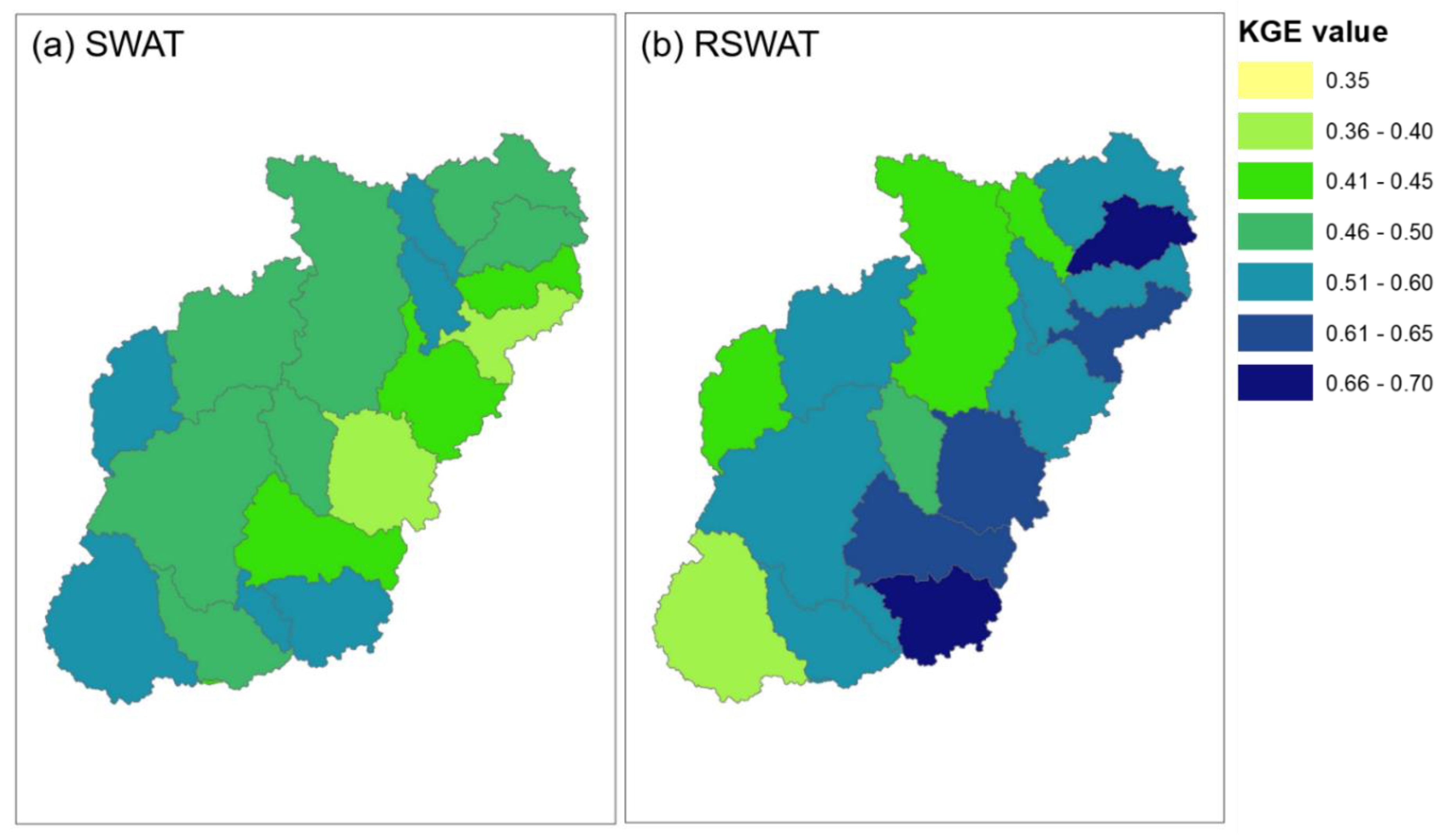
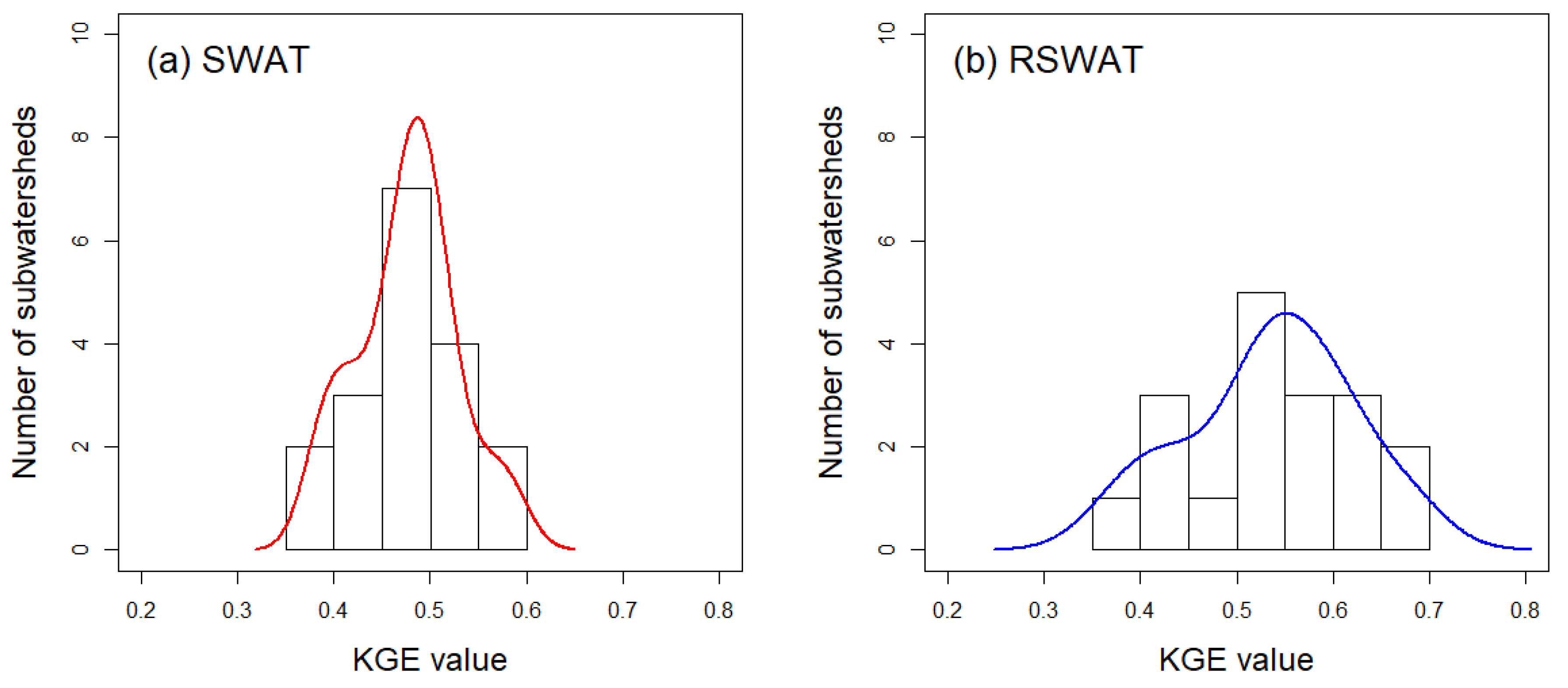
Figure 7 and Figure 8 present the KGE values from simulated ET and RS-ET for individual subwatersheds, respectively. Overall, RSWAT provided accurate ET prediction results with higher KGE values than SWAT. The average KGE values of SWAT and RSWAT were 0.47 (0.38–0.58) and 0.53 (0.37–0.68), respectively. Some of the subwatersheds showed higher KGE values in SWAT than in RSWAT (Figure 6), potentially due to the direct use of watershed level calibration results. A subwatershed-level calibration may better represent the performance of RSWAT over SWAT. Rajib et al. [61] assessed subwatershed-level ET predictions using four different model configurations, finding that the KGEs ranged from 0.35 to 0.8. Compared to this study, Rajib et al. [61] had higher KGEs; this may be because parameters were adjusted for individual subwatersheds and a greater number of parameters affecting ET were considered [62]. However, the size of our study site was too small to conduct a subwatershed-level calibration. Becker et al. [60] conducted model calibration at a scale smaller than the subwatershed scale, finding that the average KGE (0.4) was relatively low; such assessments may fail to show improved model predictions. As per Becker et al. [60], model calibration at the finest spatial level (i.e., HRU) may be unsuitable when RS-ET is utilized, as the size and configuration of the HRU is extremely random for comparisons with RS-ET [60]. Conversion of HRU ET results to a grid was found as a promising way to make comparison between SWAT results and grid-format ET, but a grid size should be carefully selected [69]. The approach adopted in this study is considered reasonable to address our aim; however, the inclusion of parameters associated with ET is recommended for future studies.
Overall, subwatershed-level metrics better quantified model improvements relative to the watershed level metrics. Spatial pattern evaluation using remotely sensed data was reported as a promising means to reveal improved model performance [70]. It is recommended that future studies that adopt remotely sensed data should use finer spatial scale metrics to effectively discern model output improvements.
The advent of RS-ET availability has produced advances in hydrologic modeling approaches. Model calibration against RS-ET aids the prediction of future water demand for agricultural activities via the enhanced representation of water consumption by crops [71]. By being a direct constraint, RS-ET is capable of supporting studies that assess the performance of different ET calculation methods based on observed streamflow [72,73]. A previous study observed enhanced model performance through the inclusion of RS-ET for multi-objective model calibration [74]. Wambura et al. [13] set up RS-ET as an additional constraint in conjunction with a primary constraint (streamflow), concluding that the addition of RS-ET reduced equifinality and predictive uncertainty. Parajuli et al. [75] demonstrated that model calibration based on RS-ET may be used to characterize hydrologic cycles in regions with limited meteorological data. Spatial calibration informed by RS-ET can increase overall model prediction accuracy [61]. The results from this study also demonstrate the value of RS-ET in assessing improved model structures, suggesting the added potential of RS-ET in advancing hydrologic modeling.
To better substantiate these findings, various improved model structures need to be tested with remotely sensed data in landscapes with different topographic and climatic conditions. As previously stated in the introduction section, ET is a key component of hydrologic cycling. The use of RS-ET in hydrologic modeling is able to better characterize hydrologic dynamics in various landscapes. In conjunction with RS-ET, remotely sensed hydrologic data, including soil moisture [76], is becoming increasingly available. This new data source provides opportunities for hydrologic modelers to better understand hydrologic processes, establish spatially explicit parameters, assess model performance, and improve the capacity of hydrologic modeling tools for water resource management. Efforts to integrate remotely sensed data into hydrologic models will increase the credibility of modeled outputs in operational applications.

4. Conclusions

We employed RS-ET to evaluate the predictive capability of a modified SWAT (i.e., the RSWAT) that contains improved representation of soil moisture dynamics. Streamflow and watershed-level RS-ET were used to calibrate SWAT and RSWAT. Simulations with the best performance metrics from the two models (i.e., SWAT and RSWAT) were compared at the watershed and subwatershed levels. The comparisons were made to determine the model that best predicted streamflow and watershed-level ET, and to understand to what extent the two models depict subwatershed-level ET. For subwatershed-level comparisons, RS-ET was divided by the subwatershed boundary and then compared with the subwatershed-level simulated ET. Three metrics (NSE, P-bias, and KGE) and one metric (KGE) were used to assess model predictability for streamflow and ET, respectively. There were two keys findings from the results of this assessment. First, SWAT and RSWAT produced similar streamflow and ET at the watershed level with similar performance metrics. NSE, P-bias, and KGE for daily streamflow were 0.47, 0.29, and 1.7% (SWAT) and 0.49, 0.37, and 15.9% (RSWAT), respectively. SWAT and RSWAT had KGE values of 0.48 and 0.52 for daily ET, respectively. Second, differences between SWAT and RSWAT were more evident at the subwatershed level. RSWAT demonstrated increased prediction accuracy in most subwatersheds relative to SWAT, with greater average KGEs (i.e., average KGE values of 0.47 and 0.53 for SWAT and RSWAT, respectively). Previous studies that demonstrate model improvements using observations at the watershed outlet often failed to show significant improvements of model predictions caused by upgrading model structures based on the performance metrics mainly owing to limited observational data [28,29]. However, our study overcame this limitation by inclusion of RS-ET, leading to improved disparity of the performance metric between existing and modified SWATs. These findings demonstrate that the use of RS-ET as a further model constraint improves the ability to discern model prediction quality attributable to model structure improvements. Subwatershed-level metric comparisons reinforce the value of RS-ET data in informing the calibration process and discerning differences in model structure performance. Therefore, our study emphasizes the applicable way of remotely sensed data to support hydrologic models, being toward generating results approximating the realistic conditions.

Author Contributions

S.L. conducted most of the analysis and writing; J.Q. and X.Z. provided technical support for modeling; H.K. assisted with the interpretation of results; M.A. provided the key dataset for model calibration and validation; G.W.M., G.E.M., and L.D. contributed to manuscript review and editing. All authors provided useful comments and suggestions for manuscript revision. All authors have read and agreed to the published version of the manuscript.

Funding

This work was supported by: (1) the United States Department of Agriculture (USDA) Natural Resources Conservation Service in association with the Wetland Component of the National Conservation Effects Assessment Project; (2) the USDA National Institute of Food and Agriculture (NIFA, 2017-67003-26484 and 2017-67003-26485); and (3) the NASA Terrestrial Ecology Program (NNX17AE66G). Hyunglok Kim was supported in part by the Future Investigators in NASA Earth and Space Science and Technology (FINESST) under Award #80NSSC19K1337.

Conflicts of Interest

The authors declare no conflict of interest.

References

  1. Cosgrove, W.J.; Loucks, D.P. Water management: Current and future challenges and research directions. Water Resour. Res. 2015, 4823–4839. [Google Scholar] [CrossRef] [Green Version]
  2. Brown, C.M.; Lund, J.R.; Cai, X.; Reed, P.M.; Zagona, E.A.; Ostfeld, A.; Hall, J.; Characklis, G.W.; Yu, W.; Brekke, L. The future of water resources systems analysis: Toward a scientific framework for sustainable water management. Water Resour. Res. 2015, 51, 6110–6124. [Google Scholar] [CrossRef]
  3. Poff, N.L.; Brown, C.M.; Grantham, T.E.; Matthews, J.H.; Palmer, M.A.; Spence, C.M.; Wilby, R.L.; Haasnoot, M.; Mendoza, G.F.; Dominique, K.C.; et al. Sustainable water management under future uncertainty with eco-engineering decision scaling. Nat. Clim. Chang. 2016, 25–34. [Google Scholar] [CrossRef] [Green Version]
  4. Devia, G.K.; Ganasri, B.P.; Dwarakish, G.S. A Review on Hydrological Models. Aquat. Procedia 2015, 4, 1001–1007. [Google Scholar] [CrossRef]
  5. Kirchner, J.W. Getting the right answers for the right reasons: Linking measurements, analyses, and models to advance the science of hydrology. Water Resour. Res. 2006, 42, W03S04. [Google Scholar] [CrossRef]
  6. Farmer, W.H.; Vogel, R.M. On the deterministic and stochastic use of hydrologic models. Water Resour. Res. 2016, 52, 5619–5633. [Google Scholar] [CrossRef] [Green Version]
  7. Whittaker, G.; Confesor, R.; Di Luzio, M.; Arnold, J.G. Detection of overparameterization and overfitting in an automatic calibration of SWAT. Trans. ASABE 2010, 53, 1487–1499. [Google Scholar] [CrossRef]
  8. Beven, K. Towards an alternative blueprint for a physically based digitally simulated hydrologic response modelling system. Hydrol. Process. 2002, 16, 189–206. [Google Scholar] [CrossRef] [Green Version]
  9. Yan, B.; Fang, N.F.; Zhang, P.C.; Shi, Z.H. Impacts of land use change on watershed streamflow and sediment yield: An assessment using hydrologic modelling and partial least squares regression. J. Hydrol. 2013, 484, 26–37. [Google Scholar] [CrossRef]
  10. Yen, H.; Bailey, R.T.; Arabi, M.; Ahmadi, M.; White, M.J.; Arnold, J.G. The Role of Interior Watershed Processes in Improving Parameter Estimation and Performance of Watershed Models. J. Environ. Qual. 2014, 43, 1601–1613. [Google Scholar] [CrossRef] [PubMed]
  11. Seibert, J.; McDonnell, J.J. On the dialog between experimentalist and modeler in catchment hydrology: Use of soft data for multicriteria model calibration. Water Resour. Res. 2002, 38, 1241. [Google Scholar] [CrossRef]
  12. Arnold, J.G.; Youssef, M.A.; Yen, H.; White, M.J.; Sheshukov, A.Y.; Sadeghi, A.M.; Moriasi, D.N.; Steiner, J.L.; Amatya, D.M.; Skaggs, R.W.; et al. Hydrological processes and model representation: Impact of soft data on calibration. Trans. ASABE 2015, 58, 1637–1660. [Google Scholar] [CrossRef]
  13. Wambura, F.J.; Dietrich, O.; Lischeid, G. Improving a distributed hydrological model using evapotranspiration-related boundary conditions as additional constraints in a data-scarce river basin. Hydrol. Process. 2018, 32, 759–775. [Google Scholar] [CrossRef]
  14. Lee, S.; Yeo, I.-Y.; Lang, M.W.; McCarty, G.W.; Sadeghi, A.M.; Sharifi, A.; Jin, H.; Liu, Y. Improving the catchment scale wetland modeling using remotely sensed data. Environ. Model. Softw. 2019, 122, 104069. [Google Scholar] [CrossRef]
  15. Sharifi, A.; Lang, M.W.; McCarty, G.W.; Sadeghi, A.M.; Lee, S.; Yen, H.; Rabenhorst, M.C.; Jeong, J.; Yeo, I.-Y. Improving model prediction reliability through enhanced representation of wetland soil processes and constrained model auto calibration—A paired watershed study. J. Hydrol. 2016, 541, 1088–1103. [Google Scholar] [CrossRef] [Green Version]
  16. Rajib, A.; Kim, I.L.; Golden, H.E.; Lane, C.R.; Kumar, S.V.; Yu, Z.; Jeyalakshmi, S. Watershed modeling with remotely sensed big data: Modis leaf area index improves hydrology and water quality predictions. Remote Sens. 2020, 12, 2148. [Google Scholar] [CrossRef] [PubMed]
  17. Carvalho-Santos, C.; Marcos, B.; Nunes, J.P.; Regos, A.; Palazzi, E.; Terzago, S.; Monteiro, A.T.; Honrado, J.P. Hydrological impacts of large fires and future climate: Modeling approach supported by satellite data. Remote Sens. 2019, 11, 2823. [Google Scholar] [CrossRef] [Green Version]
  18. Tobin, K.J.; Bennett, M.E. Improving SWAT model calibration using soil MERGE (SMERGE). Water 2020, 12, 2039. [Google Scholar] [CrossRef]
  19. Khatami, S.; Peel, M.C.; Peterson, T.J.; Western, A.W. Equifinality and Flux Mapping: A New Approach to Model Evaluation and Process Representation Under Uncertainty. Water Resour. Res. 2019, 55, 8922–8941. [Google Scholar] [CrossRef]
  20. Cho, K.H.; Pachepsky, Y.A.; Kim, J.H.; Kim, J.W.; Park, M.H. The modified SWAT model for predicting fecal coliforms in the Wachusett Reservoir Watershed, USA. Water Res. 2012, 46, 4750–4760. [Google Scholar] [CrossRef] [PubMed]
  21. Qi, J.; Li, S.; Li, Q.; Xing, Z.; Bourque, C.P.A.; Meng, F.R. A new soil-temperature module for SWAT application in regions with seasonal snow cover. J. Hydrol. 2016, 538, 863–877. [Google Scholar] [CrossRef]
  22. Nguyen, V.T.; Dietrich, J. Modification of the SWAT model to simulate regional groundwater flow using a multicell aquifer. Hydrol. Process. 2018, 32, 939–953. [Google Scholar] [CrossRef]
  23. Qi, J.; Zhang, X.; Lee, S.; Moglen, G.E.; Sadeghi, A.M.; McCarty, G.W. A coupled surface water storage and subsurface water dynamics model in SWAT for characterizing hydroperiod of geographically isolated wetlands. Adv. Water Resour. 2019, 131, 103380. [Google Scholar] [CrossRef]
  24. Liu, Y.; Yang, W.; Wang, X. Development of a SWAT extension module to simulate riparian wetland hydrologic processes at a watershed scale. Hydrol. Process. 2008, 22, 2901–2915. [Google Scholar] [CrossRef]
  25. Qi, J.; Du, X.; Zhang, X.; Lee, S.; Wu, Y.; Deng, J.; Moglen, G.E.; Sadeghi, A.M.; McCarty, G.W. Modeling riverine dissolved and particulate organic carbon fluxes from two small watersheds in the northeastern United States. Environ. Model. Softw. 2020, 124, 104601. [Google Scholar] [CrossRef]
  26. Qi, J.; Zhang, X.; Lee, S.; Wu, Y.; Moglen, G.E.; McCarty, G.W. Modeling sediment diagenesis processes on riverbed to better quantify aquatic carbon fluxes and stocks in a small watershed of the Mid-Atlantic region. Carbon Balance Manag. 2020, 15, 1–14. [Google Scholar] [CrossRef] [PubMed]
  27. Zhu, S.; Du, X.; Luo, W. Incorporation of the simplified equilibrium temperature approach in a hydrodynamic and water quality model—CE-QUAL-W2. Water Sci. Technol. Water Supply 2019, 19, 156–164. [Google Scholar] [CrossRef]
  28. Evenson, G.R.; Golden, H.E.; Lane, C.R.; D’Amico, E. Geographically isolated wetlands and watershed hydrology: A modified model analysis. J. Hydrol. 2015, 529, 240–256. [Google Scholar] [CrossRef] [Green Version]
  29. Qi, J.; Lee, S.; Zhang, X.; Yang, Q.; McCarty, G.W.; Moglen, G.E. Effects of surface runoff and infiltration partition methods on hydrological modeling: A comparison of four schemes in two watersheds in the Northeastern US. J. Hydrol. 2020, 581, 124415. [Google Scholar] [CrossRef]
  30. Kuczera, G.; Mroczkowski, M. Assessment of hydrologic parameter uncertainty and the worth of multiresponse data. Water Resour. Res. 1998, 34, 1481–1489. [Google Scholar] [CrossRef]
  31. Lee, S.; McCarty, W.G.; Lang, W.M.; Li, X. Overview of the USDA Mid-Atlantic regional wetland conservation effects assessment project. J. Soil Water Conserv. 2020, 75, 684–694. [Google Scholar] [CrossRef]
  32. Hively, W.D.; Lee, S.; Sadeghi, A.M.; McCarty, G.W.; Lamb, B.T.; Soroka, A.; Keppler, J.; Yeo, I.Y.; Moglen, G.E. Estimating the effect of winter cover crops on nitrogen leaching using cost-share enrollment data, satellite remote sensing, and Soil and Water Assessment Tool (SWAT) modeling. J. Soil Water Conserv. 2020, 75, 362–375. [Google Scholar] [CrossRef]
  33. Qi, J.; Zhang, X.; McCarty, G.W.; Sadeghi, A.M.; Cosh, M.H.; Zeng, X.; Gao, F.; Daughtry, C.S.T.; Huang, C.; Lang, M.W.; et al. Assessing the performance of a physically-based soil moisture module integrated within the Soil and Water Assessment Tool. Environ. Model. Softw. 2018, 109, 329–341. [Google Scholar] [CrossRef]
  34. Oki, T.; Kanae, S. Global hydrological cycles and world water resources. Science 2006, 1068–1072. [Google Scholar] [CrossRef] [PubMed] [Green Version]
  35. Wagener, T.; Sivapalan, M.; Troch, P.; Woods, R. Catchment Classification and Hydrologic Similarity. Geogr. Compass 2007, 1, 901–931. [Google Scholar] [CrossRef]
  36. Yeo, I.-Y.; Lee, S.; Sadeghi, A.M.; Beeson, P.C.; Hively, W.D.; McCarty, G.W.; Lang, M.W. Assessing winter cover crop nutrient uptake efficiency using a water quality simulation model. Hydrol. Earth Syst. Sci. 2014, 18, 5239–5253. [Google Scholar] [CrossRef] [Green Version]
  37. Lee, S.; McCarty, G.W.; Moglen, G.E.; Lang, M.W.; Nathan Jones, C.; Palmer, M.; Yeo, I.-Y.; Anderson, M.; Sadeghi, A.M.; Rabenhorst, M.C. Seasonal drivers of geographically isolated wetland hydrology in a low-gradient, Coastal Plain landscape. J. Hydrol. 2020, 583, 124608. [Google Scholar] [CrossRef]
  38. Wolman, M.G. Water for Maryland’s Future: What We Must Do Today; Maryland Department of the Environment: Baltimore, MD, USA, 2008.
  39. Lee, S.; Sadeghi, A.M.; McCarty, G.W.; Baffaut, C.; Lohani, S.; Duriancik, L.F.; Thompson, A.; Yeo, I.-Y.; Wallace, C. Assessing the suitability of the Soil Vulnerability Index (SVI) on identifying croplands vulnerable to nitrogen loss using the SWAT model. Catena 2018, 167. [Google Scholar] [CrossRef]
  40. Neitsch, S.; Arnold, J.; Kiniry, J.; Williams, J. Soil & Water Assessment Tool Theoretical Documentation Version 2009; Texas Water Resources Institute: College Station, TX, USA, 2011.
  41. Patankar, S.V. Numerical Heat Transfer and Fluid Flow; CRC Press: Boca Raton, FL, USA, 1980. [Google Scholar]
  42. Oleson, K.; Bonan, G.B.; Levis, S.; Thornton, P.; Vertenstein, M.; Yang, Z. Technical Description of the Community Land Model (CLM); National Center for Atmospheric Research: Boulder, CO, USA, 2004. [Google Scholar]
  43. Clapp, R.B.; Hornberger, G.M. Empirical equations for some soil hydraulic properties. Water Resour. Res. 1978, 14, 601–604. [Google Scholar] [CrossRef] [Green Version]
  44. Cosby, B.J.; Hornberger, G.M.; Clapp, R.B.; Ginn, T.R. A Statistical Exploration of the Relationships of Soil Moisture Characteristics to the Physical Properties of Soils. Water Resour. Res. 1984, 20, 682–690. [Google Scholar] [CrossRef] [Green Version]
  45. Zeng, X.; Decker, M. Improving the numerical solution of soil moisture-based Richards equation for land models with a deep or shallow water table. J. Hydrometeorol. 2009, 10, 308–319. [Google Scholar] [CrossRef]
  46. Xia, Y.; Mitchell, K.; Ek, M.; Cosgrove, B.; Sheffield, J.; Luo, L.; Alonge, C.; Wei, H.; Meng, J.; Livneh, B.; et al. Continental-scale water and energy flux analysis and validation for North American Land Data Assimilation System project phase 2 (NLDAS-2): 2. Validation of model-simulated streamflow. J. Geophys. Res. Atmos. 2012, 117, 1–27. [Google Scholar] [CrossRef]
  47. Lee, S.; Yeo, I.-Y.; Sadeghi, A.M.; McCarty, G.W.; Hively, W.D.; Lang, M.W. Impacts of watershed characteristics and crop rotations on winter cover crop nitrate-nitrogen uptake capacity within agricultural watersheds in the Chesapeake Bay region. PLoS ONE 2016, 11, e0157637. [Google Scholar] [CrossRef] [PubMed]
  48. Sun, L.; Anderson, M.C.; Gao, F.; Hain, C.; Alfieri, J.G.; Sharifi, A.; McCarty, G.W.; Yang, Y.; Yang, Y.; Kustas, W.P.; et al. Investigating water use over the Choptank River Watershed using a multisatellite data fusion approach. Water Resour. Res. 2017, 53, 5298–5319. [Google Scholar] [CrossRef] [Green Version]
  49. Anderson, M.C.; Norman, J.M.; Diak, G.R.; Kustas, W.P.; Mecikalski, J.R. A two-source time-integrated model for estimating surface fluxes using thermal infrared remote sensing. Remote Sens. Environ. 1997, 60, 195–216. [Google Scholar] [CrossRef]
  50. Anderson, M.C.; Norman, J.M.; Mecikalski, J.R.; Otkin, J.A.; Kustas, W.P. A climatological study of evapotranspiration and moisture stress across the continental United States based on thermal remote sensing: 1. Model formulation. J. Geophys. Res. Atmos. 2007, 112, D10117. [Google Scholar] [CrossRef]
  51. Arnold, J.G.; Moriasi, D.N.; Gassman, P.W.; Abbaspour, K.C.; White, M.J.; Srinivasan, R.; Santhi, C.; Harmel, R.D.; Van Griensven, A.; Van Liew, M.W.; et al. SWAT: Model use, calibration, and validation. Trans. ASABE 2012, 55, 1491–1508. [Google Scholar] [CrossRef]
  52. Yeo, I.-Y.; Lee, S.; Lang, M.W.; Yetemen, O.; McCarty, G.W.; Sadeghi, A.M.; Evenson, G. Mapping landscape-level hydrological connectivity of headwater wetlands to downstream waters: A catchment modeling approach—Part 2. Sci. Total Environ. 2019, 653, 1557–1570. [Google Scholar] [CrossRef]
  53. Ficklin, D.L.; Barnhart, B.L. SWAT hydrologic model parameter uncertainty and its implications for hydroclimatic projections in snowmelt-dependent watersheds. J. Hydrol. 2014, 519, 2081–2090. [Google Scholar] [CrossRef] [Green Version]
  54. Gupta, H.V.; Kling, H.; Yilmaz, K.K.; Martinez, G.F. Decomposition of the mean squared error and NSE performance criteria: Implications for improving hydrological modelling. J. Hydrol. 2009, 377, 80–91. [Google Scholar] [CrossRef] [Green Version]
  55. Moriasi, D.N.; Arnold, J.G.; Van Liew, M.W.; Bingner, R.L.; Harmel, R.D.; Veith, T.L. Model Evaluation Guidelines for Systematic Quantification of Accuracy in Watershed Simulations. Trans. ASABE 2007, 50, 885–900. [Google Scholar] [CrossRef]
  56. Records, R.M.; Arabi, M.; Fassnacht, S.R.; Duffy, W.G.; Ahmadi, M.; Hegewisch, K.C. Climate change and wetland loss impacts on a western river’s water quality. Hydrol. Earth Syst. Sci. 2014, 18, 4509–4527. [Google Scholar] [CrossRef] [Green Version]
  57. Zambrano, M.B. Package “hydroGOF”: Goodness-of-Fit Functions for Comparison of Simulated and Observed Hydrological Time Series. R Packag. version 0.3-8. 2017. Available online: http://www.rforge.net/hydroGOF/ (accessed on 23 February 2021).
  58. Winchell, M.; Srinivasan, R.; Di Luzio, M.; Arnold, J. ArcSWAT Interface for SWAT 2005: User’s Guide; Texas Agricultural Experiment Station and Agricultural Research Service-US Department of Agriculture: Temple, TX, USA, 2007.
  59. Poméon, T.; Diekkrüger, B.; Springer, A.; Kusche, J.; Eicker, A. Multi-objective validation of SWAT for sparsely-gaugedWest African river basins—A remote sensing approach. Water 2018, 10, 451. [Google Scholar] [CrossRef] [Green Version]
  60. Becker, R.; Koppa, A.; Schulz, S.; Usman, M.; Aus der Beek, T.; Schüth, C. Spatially distributed model calibration of a highly managed hydrological system using remote sensing-derived ET data. J. Hydrol. 2019, 577, 123944. [Google Scholar] [CrossRef]
  61. Rajib, A.; Evenson, G.R.; Golden, H.E.; Lane, C.R. Hydrologic model predictability improves with spatially explicit calibration using remotely sensed evapotranspiration and biophysical parameters. J. Hydrol. 2018, 567, 668–683. [Google Scholar] [CrossRef] [PubMed]
  62. Yang, Q.; Zhang, X. Improving SWAT for simulating water and carbon fluxes of forest ecosystems. Sci. Total Environ. 2016, 569–570, 1478–1488. [Google Scholar] [CrossRef] [PubMed] [Green Version]
  63. Sinnathamby, S.; Douglas-Mankin, K.R.; Craige, C. Field-scale calibration of crop-yield parameters in the Soil and Water Assessment Tool (SWAT). Agric. Water Manag. 2017, 180, 61–69. [Google Scholar] [CrossRef] [Green Version]
  64. Tasdighi, A.; Arabi, M.; Harmel, D. A probabilistic appraisal of rainfall-runoff modeling approaches within SWAT in mixed land use watersheds. J. Hydrol. 2018, 564, 476–489. [Google Scholar] [CrossRef]
  65. Qi, J.; Wang, Q.; Zhang, X. On the use of NLDAS2 weather data for hydrologic modeling in the Upper Mississippi River Basin. Water 2019, 11, 960. [Google Scholar] [CrossRef] [Green Version]
  66. Shahrban, M.; Walker, J.P.; Wang, Q.J.; Robertson, D.E. On the importance of soil moisture in calibration of rainfall–runoff models: Two case studies. Hydrol. Sci. J. 2018, 63, 1292–1312. [Google Scholar] [CrossRef] [Green Version]
  67. Yeo, I.-Y.; Lang, M.W.; Lee, S.; McCarty, G.W.; Sadeghi, A.M.; Yetemen, O.; Huang, C. Mapping landscape-level hydrological connectivity of headwater wetlands to downstream waters: A geospatial modeling approach—Part 1. Sci. Total Environ. 2019, 653, 1546–1556. [Google Scholar] [CrossRef] [PubMed]
  68. Tobin, K.J.; Bennett, M.E. Improving alpine summertime streamflow simulations by the incorporation of evapotranspiration data. Water 2019, 11, 112. [Google Scholar] [CrossRef] [Green Version]
  69. Abiodun, O.O.; Guan, H.; Post, V.E.A.; Batelaan, O. Comparison of MODIS and SWAT evapotranspiration over a complex terrain at different spatial scales. Hydrol. Earth Syst. Sci. 2018, 22, 2775–2794. [Google Scholar] [CrossRef] [Green Version]
  70. Mendiguren, G.; Koch, J.; Stisen, S. Spatial pattern evaluation of a calibrated national hydrological model—A remote-sensing-based diagnostic approach. Hydrol. Earth Syst. Sci. 2017, 21, 5987–6005. [Google Scholar] [CrossRef] [Green Version]
  71. Zou, M.; Kang, S.; Niu, J.; Lu, H. Untangling the effects of future climate change and human activity on evapotranspiration in the Heihe agricultural region, Northwest China. J. Hydrol. 2020, 585, 124323. [Google Scholar] [CrossRef]
  72. Aouissi, J.; Benabdallah, S.; Lili Chabaâne, Z.; Cudennec, C. Evaluation of potential evapotranspiration assessment methods for hydrological modelling with SWAT—Application in data-scarce rural Tunisia. Agric. Water Manag. 2016, 174, 39–51. [Google Scholar] [CrossRef]
  73. Chen, M.; Gassman, P.W.; Srinivasan, R.; Cui, Y.; Arritt, R. Analysis of alternative climate datasets and evapotranspiration methods for the Upper Mississippi River Basin using SWAT within HAWQS. Sci. Total Environ. 2020, 720, 137562. [Google Scholar] [CrossRef] [PubMed]
  74. Herman, M.R.; Nejadhashemi, A.P.; Abouali, M.; Hernandez-Suarez, J.S.; Daneshvar, F.; Zhang, Z.; Anderson, M.C.; Sadeghi, A.M.; Hain, C.R.; Sharifi, A. Evaluating the role of evapotranspiration remote sensing data in improving hydrological modeling predictability. J. Hydrol. 2018, 556, 39–49. [Google Scholar] [CrossRef]
  75. Parajuli, P.B.; Jayakody, P.; Ouyang, Y. Evaluation of Using Remote Sensing Evapotranspiration Data in SWAT. Water Resour. Manag. 2018, 32, 985–996. [Google Scholar] [CrossRef]
  76. Kim, H.; Parinussa, R.; Konings, A.G.; Wagner, W.; Cosh, M.H.; Lakshmi, V.; Zohaib, M.; Choi, M. Global-scale assessment and combination of SMAP with ASCAT (active) and AMSR2 (passive) soil moisture products. Remote Sens. Environ. 2018, 204, 260–275. [Google Scholar] [CrossRef]
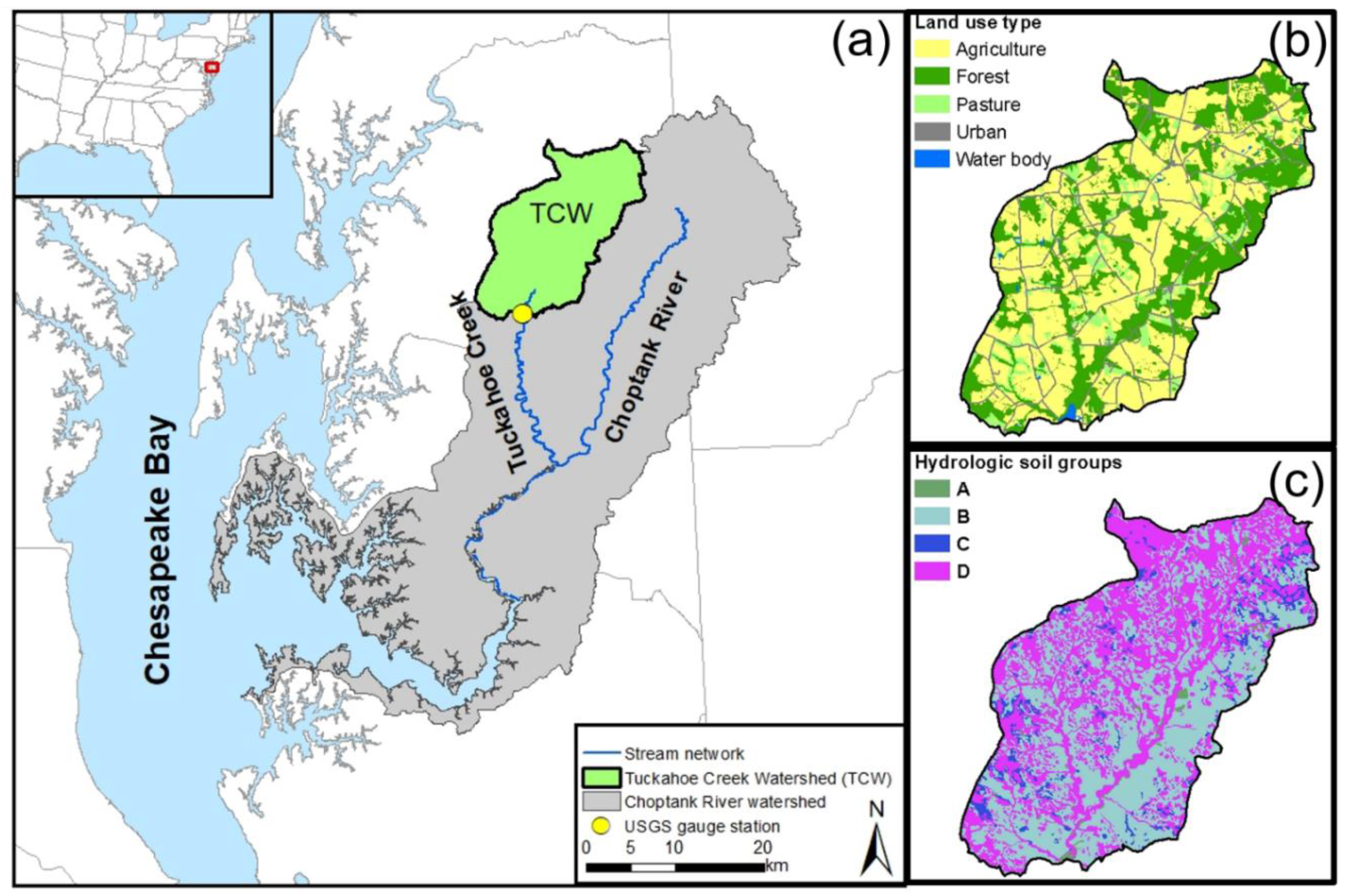
Figure 1. Characteristics of the study area (Tuckahoe Creek Watershed): (a) location; (b) land use type; and (c) hydrologic soil groups (HSGs; adapted from Lee et al. [39]) Note: HSGs are characterized as follows: type A are well-drained soils with a water infiltration rate of 7.6–11.4 mm·h−1; type B are moderately well-drained soils with 3.8–7.6 mm·h−1; type C are moderately poorly-drained soils with 1.3–3.8 mm·h−1; and type D are poorly-drained soils with 0–1.3 mm·h−1 [40].
Sustainability 13 02375 g001
Figure 2. Schematic of the Richards equation-based soil moisture module integrated with the Soil and Water Assessment Tool (SWAT) surface, infiltration, evapotranspiration (ET), and lateral flow components.
Sustainability 13 02375 g002
Figure 3. Examples of remotely sensed evapotranspiration (RS-ET) from ALEXI/DisALEXI on (a) 10 January 2013; and (b) 30 August 2013.
Sustainability 13 02375 g003
Figure 4. Flow diagram of this study.
Sustainability 13 02375 g004
Figure 5. Comparisons of daily observations (solid gray line), and simulations from SWAT (solid red line) and RSWAT (dotted blue line): (a) streamflow and (b) ET.
Sustainability 13 02375 g005
Figure 6. Flow duration curves for daily observations (solid gray line), and simulations from SWAT (solid red line) and RSWAT (dotted blue line).
Sustainability 13 02375 g006
Figure 7. Spatial distribution of subwatershed-level Kling–Gupta Efficiency (KGE) values for ET simulations: (a) SWAT and (b) RSWAT.
Sustainability 13 02375 g007
Figure 8. Density plots for subwatershed-level KGE values with an interval of 0.05: (a) SWAT and (b) RSWAT.
Sustainability 13 02375 g008
Table 1. List of input data.
Data TypeSourceDescriptionYear
ClimaticNLDAS2Hourly precipitation, temperature, solar radiation, wind speed, and humidity2008–2014
DEMMD-DNRLiDAR-based 1-m resolution2006
Land useUSDA-NASSCropland Data Layer (CDL)2008–2012
MRLCNational Land Cover Database (NLCD)2006
USDA-FSA-APFONational Agricultural Imagery Program digital Orthophoto quad imagery1998
US Census BureauTIGER road map2010
SoilsUSDA-NRCSSoil Survey Geographical Database (SSURGO)2012
StreamflowUSGSDaily streamflow2010–2014
ETSun et al. [48]Daily ET2010–2014
Note: NLDAS2: North American Land Data Assimilation System 2; DEM: Digital Elevation Model; MD-DNR: Maryland Department of Natural Resources; LiDAR: light detection and ranging; MRLC: Multi-Resolution Land Characteristics Consortium; USDA-FSA-APFO: USDA-Farm Service Agency-Aerial Photography Field Office; and TIGER: Topologically Integrated Geographic Encoding and Referencing.
Table 2. List of calibrated parameters.
ParameterDescription (Units)RangeSWATRSWAT
CNSCS runoff curve number−20–20%0%−3%
GW_DELAYGroundwater delay (days)0–1000.1488.63
ALPHA_BFBaseflow alpha factor (days−1)0–10.430.83
GWQMNThreshold depth of water in the shallow aquifer required for return flow to occur (mm H2O)0–500013.851226.97
GW_REVAPGroundwater “revap” coefficient0.02–0.20.170.15
REVAPMNThreshold depth of water in the shallow aquifer for “revap” to occur (mm H2O)0–500450.9568.69
SOL_AWCAvailable water capacity of the soil layer (mm H2O ·mm soil−1)−50–50%−26%−43%
CH_K2Manning’s “n” value for the main channel0–15092.07145.11
CH_N2Manning’s “n” value for the tributary channels0.01–0.30.170.03
SURLAGSurface runoff lag coefficient0.5–2422.480.85
ESCOSoil evaporation compensation factor0–10.920.69
EPCOPlant uptake compensation factor0–10.210.40
CANM#Maximum canopy storage (mm H2O)0–10.720.42
Publisher’s Note: MDPI stays neutral with regard to jurisdictional claims in published maps and institutional affiliations.