1. Introduction
Major investments in the field of transportation have several unique characteristics that differentiate them from investments in other fields of economy. Consequently, professional preparation of decisions is crucial, as investment costs are typically very high. Such projects create infrastructure with several decades of service life, and thus problems arising due to poor preparation can only be amended with a considerable amount of resources. Road safety is one of the pillars in the Sustainable Development Goals, and it does not only explicitly address the issues related to good health and safety of the people, but it is also associated with the targets towards the development of sustainable cities [
1]. Because of the scarce resources available, the implementation of the most effective road safety improvements is of paramount importance, so an analysis of each project’s effectiveness cannot be avoided [
2]. Efficiency analysis ought to apply a complex approach, including a socio-economic study [
3,
4]. Together with the financial analysis, parameters affecting a wide range of economic actors need to be involved and evaluated from several points of view. Such a determining feature is the incidence and socio-economic impact of traffic accidents.
The scarcity of widely available methodologies for defining and managing these effects in developed countries shows that the analysis of these effects is complicated, though mandatory. However, it is of utmost importance to detect areas where a transportation safety improvement will have a significant impact.
Since accidents are believed to be discrete, random, and non-negative, Poisson and negative binomial models were generally implemented (e.g., [
5]). The problem with those models is that they assume that accidents are independent of the space they occur in, although this is not the case in reality [
6]. Generally, the safety performance functions (SPF) used in international practice usually modeled by negative binomial distribution due to the typically occurring overdispersion problem, as the equations can be solved, but there is no evidence that the accident frequency indeed follows a negative binomial distribution. Thus, we aimed to take the spatial effect into account when setting up the estimator model.
While road traffic crashes tend to occur at specific times, they are also affected by a comprehensive interaction of spatial factors
[7]. The heterogeneity among traffic crashes on roads with the same geometric conditions is because of the unlikeliness of independence across space [
8].
Accidents are not randomly distributed in space but represent spatial autocorrelation [
7]. Spatial autocorrelation is the degree of influence by the value of a variable at a certain location on the value of the same variable at a contiguous location [
9].
In the literature, 36 articles have been identified that also take spatiality into account in some way when analyzing traffic accidents.
Table 1 summarizes how the literature can be classified, what explanatory variables that are relevant to us are used, and which of the most commonly used spatial econometric models (SAR—Spatial Autoregression, SEM—Spatial Error Model) appear in it.
Spatial traffic accident models that appear in the literature can be divided into three major groups according to how spatial interactions are handled: (i) the delimitation of spatial units appears, but the modeling of the interactions between them is omitted; (ii) they compare models that handle spatial interaction with models that do not take spatial interaction into account; (iii) only models that handle spatial interactions are set up. Within these, one of two approaches was used in each case: (a) the analyses are based on the elements of the line road network, within which it is delimited whether the given accident occurs at an intersection or between two intersections; (b) the analyses are based on spatial units. Based on this, the articles published in the literature can be classified as shown in
Table 2.
In the literature, 36 spatial models were identified. As
Table 1 and
Table 2 illustrate, for 31 of these, either the spatial units are the observed units (b); or they do not take into account spatial interactions (i); or they only analyze spatial models (iii). This article follows the five studies enumerated in the highlighted cell of
Table 2, as we have compared spatial and non-spatial models (ii), based on the elements of the linear road network (a), including the sections between intersections. Two of the mentioned articles deal with intersections [
24,
28]. The remaining three discuss accidents on motorways. The article by Wang et al. [
18] examines the accident frequency of the M25 motorway around London, on which they build Poisson-lognormal, Poisson-Gamma, and Poisson-lognormal CAR (conditional autoregressive) [
44] models. The range of explanatory variables includes infrastructure characteristics as well as traffic characteristics. Out of these, the Congestion Index is highlighted, but traffic volume and speed are also displayed. The article by Castro et al. [
19] deals with motorways around Austin, TX, USA, and the range of explanatory variables includes crash characteristics, highway design attributes, characteristics of drivers and vehicles involved in the crash, and environmental factors. The article by Xie et al. [
20] examines accidents caused by Hurricane Sandy according to the type of accident, where it occurred, and at what time of day.
The articles detailed above, which most closely resemble ours, take into account highway sections; thus, our analysis of urban sections fills a gap. The range of explanatory variables appears in many of the articles examined, such as traffic volume, speed, number of lanes, or length of sections (e.g., [
18]), the existence of bus lanes (e.g., [
11]), or ratio of truck traffic (e.g., [
34]). Another difference is that in addition to the traditionally used SAR and SEM approaches, Spatial Autocorrelation (SAC) [
45] models are also used. Although several articles in the literature have taken other approaches in addition to the SAR and SEM models, such as the Spatial Durbin Model (e.g., [
6,
30]) or the Besag–York–Mollié model [
46] (e.g., [
35,
36]), SAC models have not been used by anyone in the literature known to us yet. In summary, we focused on an area that is missing from the literature: joint usage of four techniques: (i) we used spatial econometric models; (ii) we used real network sections instead of other spatial units; (iii) we analyzed urban roads instead of rural area; (iv) we take into account the spatial autocorrelation (SAC) modeling technique.
The main objective of this article is to identify a proper model for estimating the accident frequencies on different sections of the road infrastructure with different properties in Budapest, Hungary (for Hungary, there are numerous traffic safety models, such as [
47,
48,
49]). Our assumption that a spatial econometric point of view could help us to create such a model.
The paper is organized as follows. The dataset and its preprocessing are described in the next chapter.
Section 3. explains the methodology employed to diagnose spatial dependence among the data. The test and model results are discussed in
Section 4, and the paper is concluded by
Section 5.
3. Methodology
The applied methodology is mostly based on the research of Luc Anselin [
52], and Attila Varga [
53]. The main idea behind the applied model environment is based on the phenomenon that traditional linear regression models estimated by ordinary least squares methods cannot take into consideration the fact that panel data based upon spatial specifications is not independent of its spatial location [
52]. This means, models in which spatial autocorrelation can be found in the linear regression errors cannot be used for further investigation; instead, a spatial econometric model ought to be used.
The spatial econometric analysis applied here follows the methodology described by [
54]. The first step is to set up the Ordinary Least Squares (OLS) models with proper explanatory variables (3).
where
y: dependent variable;
α: constant term;
βi: estimated coefficients of the linear regression model (∀j = 1..m);
xi: explanatory variables (∀j = 1..m);
ε: error term (Eεi = 0, V(εi) = σ2);
N: number of observations.
The second step is the definition of the weight matrices. In accordance with the methodology proposed in the literature [
54], queen type binary (B) matrices have been applied in our research, which are transformed into row standardized weight matrices (W). In the case of binary matrices, the spatial units have an effect on each other, depending on whether they are neighbors to each other (1) or not (0). A detailed description of this method can be found in [
52,
53,
54,
55,
56]. Two conditions of neighborhood are introduced, one is where two points of interest are neighbors to each other if they are closer than a given distance. The second is when the given point neighbors are the
k closest points (
k can be chosen arbitrarily) or
k nearest neighbors.
The third methodological step is to prove the existence of spatial autocorrelation in the dataset. The presence of spatial autocorrelation depends on the weight matrix. The existence of spatial autocorrelation and the proper weight matrix can be tested by the Moran-
I test [
57]. If the test results in a significant effect, a spatial econometric model can be applied [
53].
where
N: number of investigated points;
xi, xj: the observed value of two points of interest;
μ: the expected value of x;
wij: the elements of the spatial weight matrix;
S0: normalizer—S0 = ∑i,jwi,j
If the existence of spatial autocorrelation is proven, three types of models can be set up: the SAR, the SEM, and the SAC. In order to decide which model should be used, the Lagrange–Multiplier test is available [
54,
58]. If it can be assumed that the spatial lagged dependent variable also affects the dependent variable, the SAR model should be chosen. In this case, the following regression formula can be applied [
53]:
where
y: vector of the dependent variables;
ρ: autoregressive parameter;
W: weight matrix;
β: coefficient vector;
X: matrix of the independent variables;
ε: vector of errors (E(εi) = 0, V(εi) = σ2);
N: number of points of interest;
K: number of independent variables.
If spatial dependence can be eliminated from the model, and the spatial effects can be transferred to the error term, the SEM model should be used. In this case, the formulas presented below can be used [
53]:
where
The third option is to use the two approaches (the modeling of spatial lag, and spatial error) together. There are several models for this [
45], out of which the SAC was used, because this is the one which can handle two different weight matrices at the same time. Its formula is given in Equation (8).
After building the OLS, SAR, and SEM models, the results were compared by Akaike’s Information Criterion (
AIC) and Bayesian Information Criterion (
BIC) [
59]. In addition to
AIC and
BIC, we used the likelihood test ratio (
LR) as well. According to this approach, two hierarchical models (the superior one has one or more surplus estimated parameter) can be compared to each other based upon the ratio of their likelihood value. The test formula is given in Equation (9) [
60]:
where
L1: likelihood value of the inferior model;
L2: likelihood value of the superior model;
df: degree of freedom for the chi-square distribution, equal to the number of the surplus estimated variables.
Spatial econometric analyses were performed in the R 3.4.0 environment [
61]. The maptools [
62], sp [
63,
64], spdep [
63,
65] and spatialreg [
63,
66,
67] libraries were used during the analysis.
5. Discussion
For the SEM model, which is considered to be the best, the sign of all explanatory variables (except for the ratio of HGVs) is positive and significantly different from zero. This can be considered as obvious for the length of the examined sections or the average daily traffic because it means that the longer the given section, or the higher the traffic on it, the higher the accident frequency. For bicycle traffic volume, the same observation can be applied, as if cycling traffic is higher, the frequency of accidents also increases. This is incoherent with the models observed in Denmark or the Netherlands due to the fact that in Budapest, there is a few physically separated infrastructure for cyclists [
69], and the volume of bicycle traffic has not reached the critical level where the trend is reversed, and the risk of an accident decreases as bicycle traffic increases.
In the case of the category variables describing the characteristics of the infrastructure, it can be stated that the minimum number of accidents occurred on the high-speed seven-lane roads (this was chosen as a reference among the category variables). Generally, the frequency of accidents is lower on the road developed for higher speed, which can be derived from that these sections have a higher level of safety (guardrail, and divided road).
In the number of lanes: between 20 and 50 kph, there is no clear correlation between the number of lanes and the accident frequency; at higher speed designed sections (above 50 kph), the accident frequency decreases for more than four lanes.
In the case of parameters describing the quality of road public transport, it can be observed that the increase in bus traffic increases the risk of accidents. This is due to the fact that buses in traffic perform maneuvers that other road users do not expect (approaching and leaving a bus stop, handling overhead lines in the case of trolleybuses, and taking into account insulated sections).
The same is right for bus lanes, which, with their special rules, contribute to an increase in the risk of accidents, typically due to conflict situations resulting from pre-turn lane changes.
In the case of HGV traffic, the properties of the parameters are different from the previous ones. On the one hand, whether HGVs (over 12 tons) can use a given road section has no significant effect on the frequency of accidents. On the other hand, the ratio of HGVs negatively affects the accident frequency, i.e., the higher the proportion of HGV traffic in total traffic, the lower the frequency of accidents. This is due to the fact that lorries are less dynamic in traffic, perform less unforeseen maneuvers, and likely to use more protected main roads.
If the spatial parameters are taken into consideration, both the SAR and SEM model’s parameters are significant; however, this cannot be said about the SAC model. Both SAR and SEM models have a positive spatial parameter, which means if a section’s accident frequency is high, then the closest one’s frequency will also be increased. This indicates that improvements for longer road sections seem to be beneficial in order to avoid traffic accidents. In the case of SAC models, both spatial parameters are not significantly differentiated from zero, which can be due to the fact that the two approaches (spatial error and delay) effect cancel each other out. Since the spatial parameters are not significant in this case, the effects described above are not fulfilled in this case.
The best model with a significantly positive spatial parameter (λ) is the SEM approach. This indicates that the closest infrastructure elements have a positive effect on each other, which could be eliminated from the model. These effects can be derived from the urban structure and the geographical properties affecting the city. These parameters are hard to take into consideration in a classic linear regression; thus, it can be stated that the spatial econometric approach is a more effective technique for modeling road accident frequency.
6. Conclusions
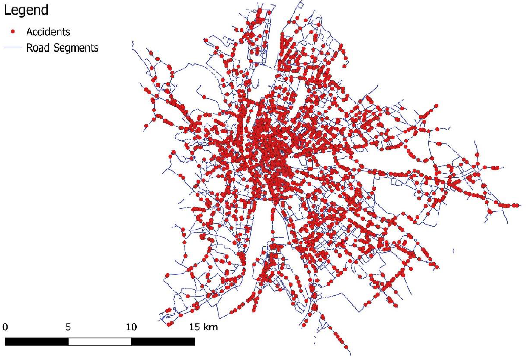
In this study, road traffic accidents occurring on the road links of Budapest over a three-year-long period were surveyed. The accidents on the same link were aggregated, and centroids of each road link were considered for the formulation of three different types of models. The global Moran’s I test results with significant p-value and positive z-score confirm the presence of spatial dependence of road traffic accidents. OLS, SAR, SEM, and SAC models were formulated in this study. The results proved that incorporating spatial effect in the model gives a better result than the traditional multiple linear regression model. The Lagrange–Multiplier test, in conjunction with the AIC, BIC, and Log-Likelihood values proved that the spatial error model gives the best output over the remaining two spatial econometric models in this study. Confirmation of spatial dependence among the data; illustration of better performance of the spatial models over traditional OLS models; and identification of significant contributors or predictors of the road traffic accidents are the main findings of this study.
The spatial econometric approach allows the development of a universal and simple model that will significantly assist decision-makers in the development of road safety investments. The role of spatial econometrics is to include difficult or non-descriptive parameters in the model, which allows for a more accurate prediction of accident frequencies. However, it is essential to update these models every 3–5 years, as there may be changes in the urban structure that will fundamentally change traffic safety conditions.
This study’s main limitation is that the analysis only takes into consideration the city of Budapest. Furthermore, it considered accident events on the road links only; those at the intersections are not considered. The third limitation is that accident severity was not considered; instead all accidents that occurred on the road links over a period are aggregated.
These limitations define the future research directions. Three main directions could be identified: (i) choosing a different environment rather than Budapest, such as an analysis on the whole Hungarian network; (ii) take into consideration the accidents of the junctions in a separate model, or a joint one as well; (iii) taking into consideration the accident types and the accident results. Developing such spatial econometric models of good performance and discovering the most significant parameters would help authorities identify the specific interventions in improving road safety and ultimately ensure sustainable transport and urban development.


