Assumptions
The location of the structure was Sydney, and the terrain category was taken to be terrain category 2. Since Sydney is in region A2, as outlined in the AS1170.2 [
22] and assuming an average recurrence interval of 500 years,
as shown in
Table 3 of AS1170.2 [
22]. Therefore, the terrain multiplier, taken from
Table 4 of AS1170.2, for a height of 3 m, was terrain/height multiplier
[
6] (pp. 19–20). The shielding multiplier,
, was taken from
Table 4 of AS1170.2 as the most conservative case [
6] (p. 21). For a better analysis, the heights of buildings in the surrounding area needed to be recorded and, utilizing clause 4.3 [
22], a detailed analysis should return a more accurate shielding multiplier value. However, given the lack of a specific location for the structure, the most conservative case was taken. The topographic multiplier,
, was taken from
Section 3.4, and lee regions were ignored as per clause 4.4.3 as no lee zones are in Australia. This was not the most conservative case, as
and
. However, because of a lack of specified location, the analysis for the topography of the site could not be analyzed. This would have been done by utilizing geospatial software to model the topography around the site and by conducting an analysis on the maximum height of hills in that region.
Calculating Wind Speed
Since
was the most conservative case,
. It should be noted, however, that a static wind analysis using the values found in AS1170.2 [
22] and utilized in previous years is not an accurate representation of wind effects on a structure over a long period of time. This is because the values utilized refer to the gust wind speed, which is a maximum wind speed event with a duration outlined in AS1170.2 [
22] as being a 0.2-s gust event. This means that structures will be over-designed to resist this maximal value for wind speeds that are unlikely to occur. This is because the wind recordings in
Table 3 are based on historical records where the maximum wind speed is taken without distinguishing whether it is from a synoptic wind or a thunderstorm event. These two wind events have different profiles and, for a smaller structure, since the standard just records the maximum event, there is the possibility that the wind speed is based on a thunderstorm event. Hence, if this was used to define the normal response to a structure for winds occurring regularly, then there would have been the potential for overdesigning of the structure. Instead, it would be more advantageous to analyze a structure’s response to a larger duration wind event.
Since a synoptic wind event is made up of two parts; a mean component and a fluctuating component, the fluctuating component is responsible for the dynamic effects induced by wind loads, and for roof structures on which the wind speeds have the most effect, due to the increasing wind speed as elevation increases, the roof is going to have the most adverse effects due to wind loading.
Using the equation,
where:
Turbulence intensity is found in
Table 6 of AS1170.2 [
22] and is a measure of the turbulence in the wind. Wind turbulences are responsible for a phenomenon known as turbulence buffeting, where the turbulence induces a dynamic response in the structure. This can occur both in the along-with-wind and the crosswind direction—
Table 7 summarizes different extracted dynamic modes in different models.
This assumed that the peak factor is based on the hourly mean wind speed, hence, the period was 1 h, or 3600 s, where:
Using the value of the peak factor in the gust factor equation and rearranging the gust wind speed equation gives: .
The values for the calculation are summarized in
Table 8:
Using Davenport’s equation for the power spectrum distribution:
where
Rearranging the Davenport equation where the pressure spectrum distribution (PSD) value is dependent on the frequency gives:
This is the spectrum for the wind speed. Utilizing the fact that the velocity component for wind speed is based on a mean and fluctuating component provides:
where
is the fluctuating component of the velocity.
Using the fact that the drag force, where:
The drag coefficient, = 1.2 (semi-cylindrical roof shape)
Density of the air, = 1.2 kg/m3
The projected area,
By squaring the value of the wind velocity, .
Since the value for (
v’(
t))
The wind force due to the mean wind speed is
and the fluctuating component is
[
7] (p. 2).
Since the fluctuating component is responsible for the dynamic effects on the building:
Since the fluctuating velocity spectrum can be written as, .
Therefore, the equation for
:
Dividing the force spectrum by the square of the area,
will result in the pressure spectrum:
Since each of the models have different values, the pressure spectrum for each model are shown below.
Pressure spectrum for model 1:
Pressure spectrum for model 2:
Pressure spectrum for model 3:
Pressure spectrum for the new model:
Table 9,
Table 10,
Table 11 and
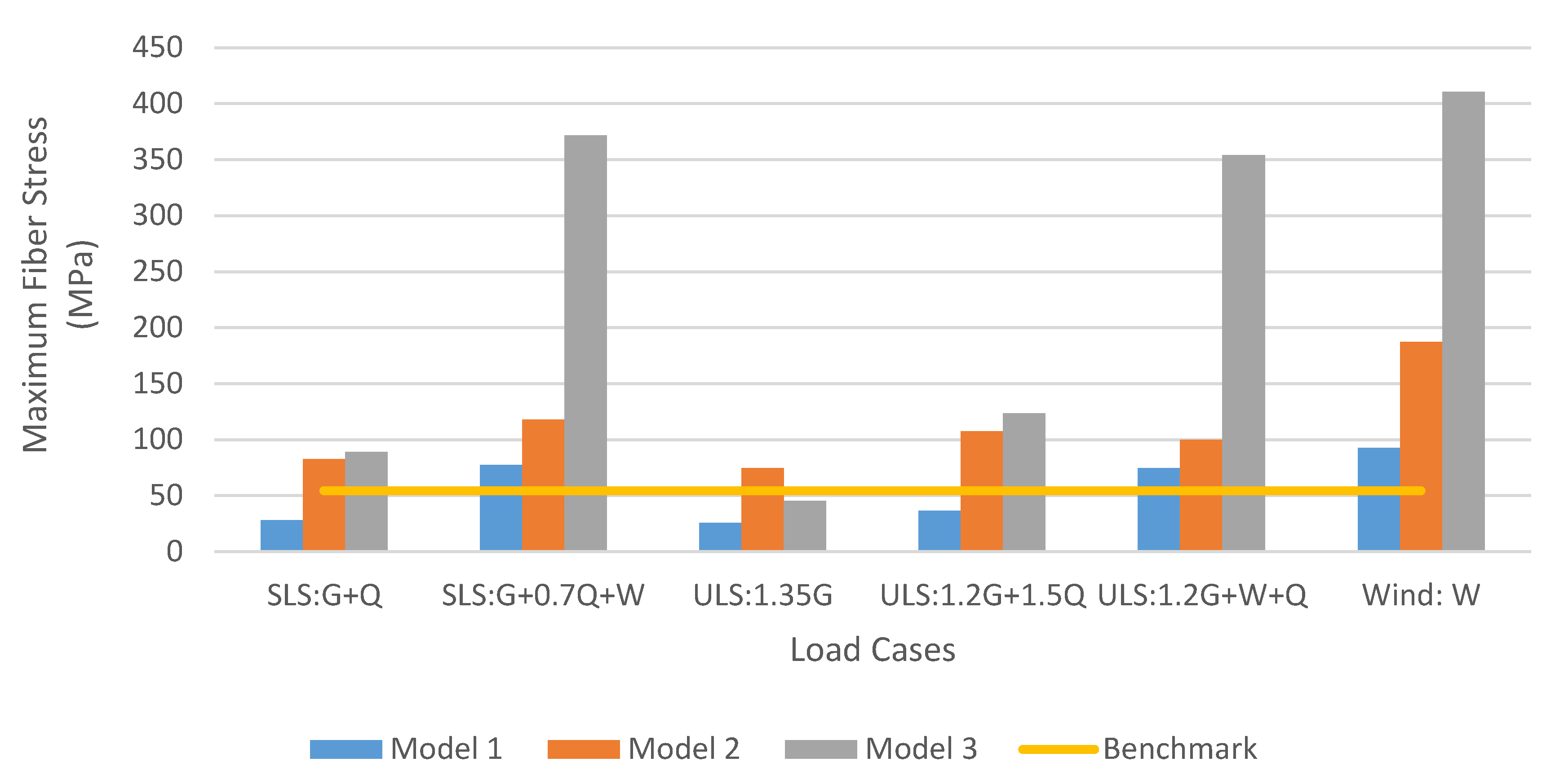
Table 12 show the classification of the main dynamic structural responses that can be extracted in different simulated models. The presented structural reactions were varied from the maximum displacement in different directions as well as the critical stresses. The presented technical values can help to provide a proper procedure in the hands of the practical engineers when it comes to designing of the light structures to meet both serviceability and ultimate requirements.
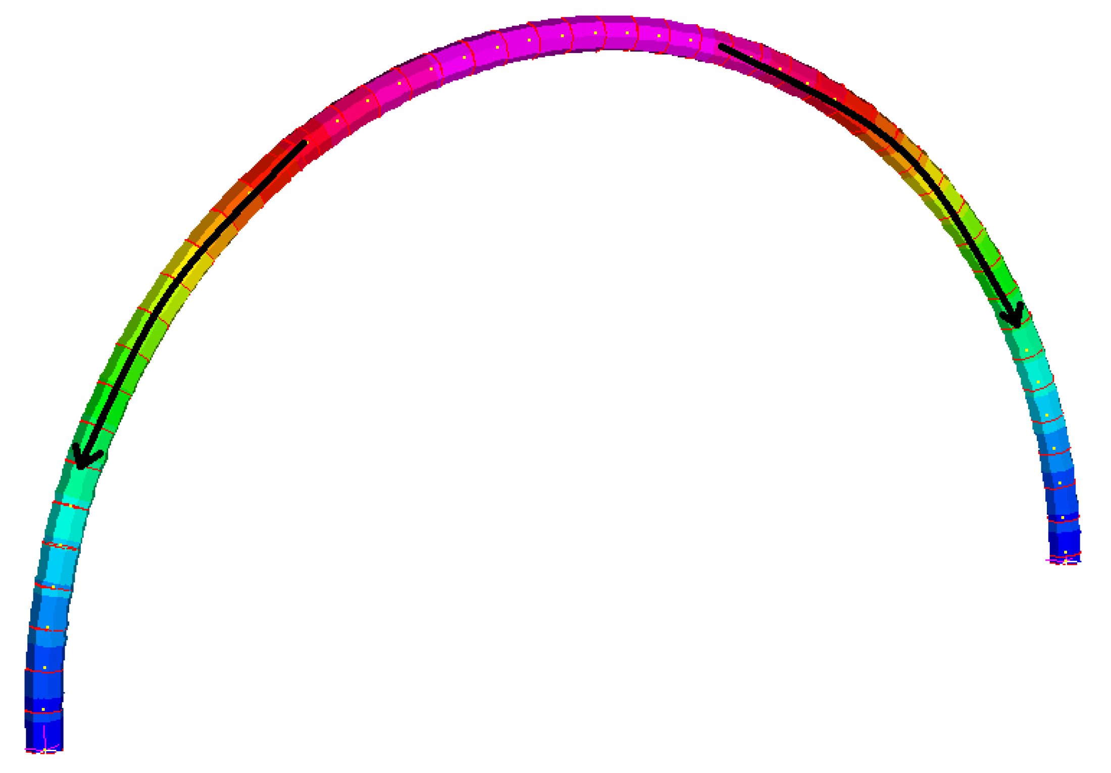
Figure 20 presents a possible model of the failure shape of model 2 due to the effect of the applied dynamic wind loading. As illustrated, a combination of bending and twisting can be found as the main failure modes in the simulated structures. The extracted modes are significantly important when it comes to designing suggested frames because of the effect of the dynamic wind loading. Additionally, the suggested concept might be extended into calculating and predicting the structural responses due to the influence of the buckling and post-buckling analysis of the simulated frames.
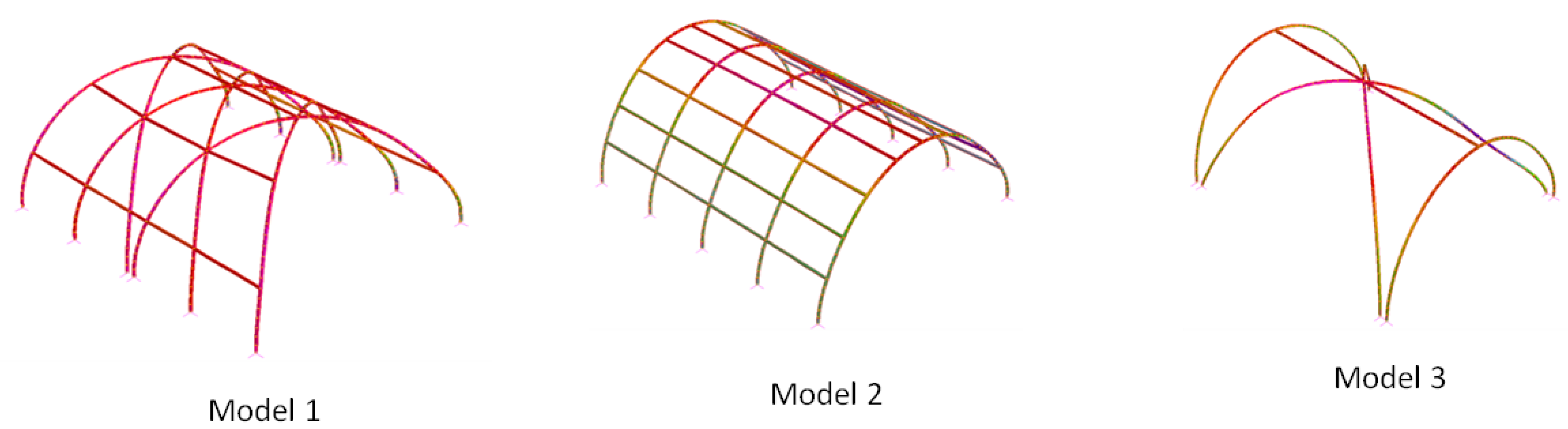
The same approach is presented in
Figure 21. Based on the simulated effect of the dynamic wind loading, which was applied to frame model 3, a combination of the shear and twisting failure modes are presented in
Figure 21. The obtained failure modes were fully dependent on the suggested shape of the frames.


 ,
, 


