
Using an Artificial Neural Networks Experiment to Assess the Links among Financial Development and Growth in Agriculture


Abstract
:1. Introduction
2. Literature Review
2.1. Productivity and Credit Access
2.2. Financial Development and Economic Growth
3. Materials and Methods
- (a)
- The development of the “neuron system” is distributed over many elements. In other words, many neurons do the same thing;
- (b)
- An address identifies each data of the algorithm used (a number), which is used to retrieve the knowledge necessary to perform a certain task;
- (c)
- ANNs, unlike standard econometric models and their software, do not have to be programmed to perform a task. ANNs learn independently based on experience or with the help of an external instructor.
| Algorithms 1. Algorithms terms to describe neural networks process |
| with each layer |
| with |
| Our NN can be written as: |
| where |
| Our activation functions can be linear or nonlinear with L = n. In the first case: |
| [11] |
| If is a linear function where . |
| If we choose, in an arbitrary way, to use a non-linear activation function, we have: |
| Thus, with rectified linear unit, we have: |
| In our NN, MSE will be: |
| In [17]: |
| Now, the Log-Likelihood (LL) will be: |
- (a)
- The development of the “neuron system” is distributed over many elements. In other words, many neurons do the same thing;
- (b)
- An address identifies each data of the algorithm used (a number), which is used to retrieve the knowledge necessary to perform a certain task;
- (c)
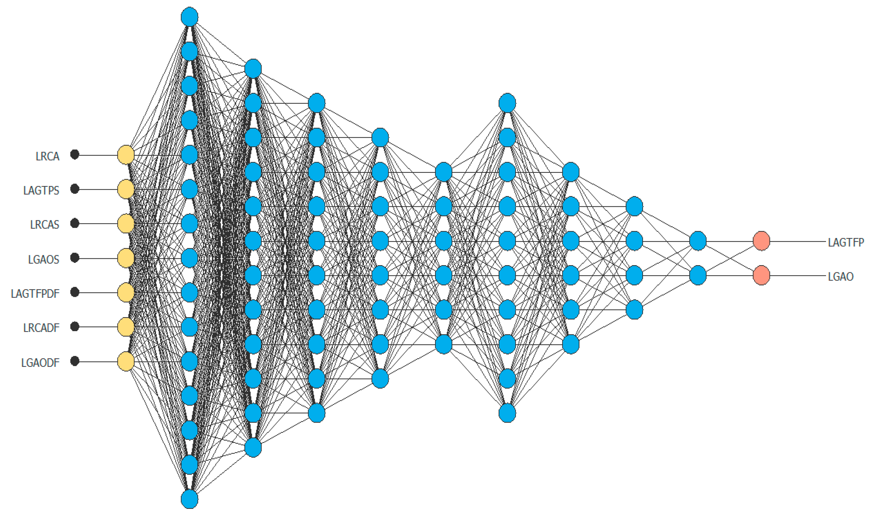
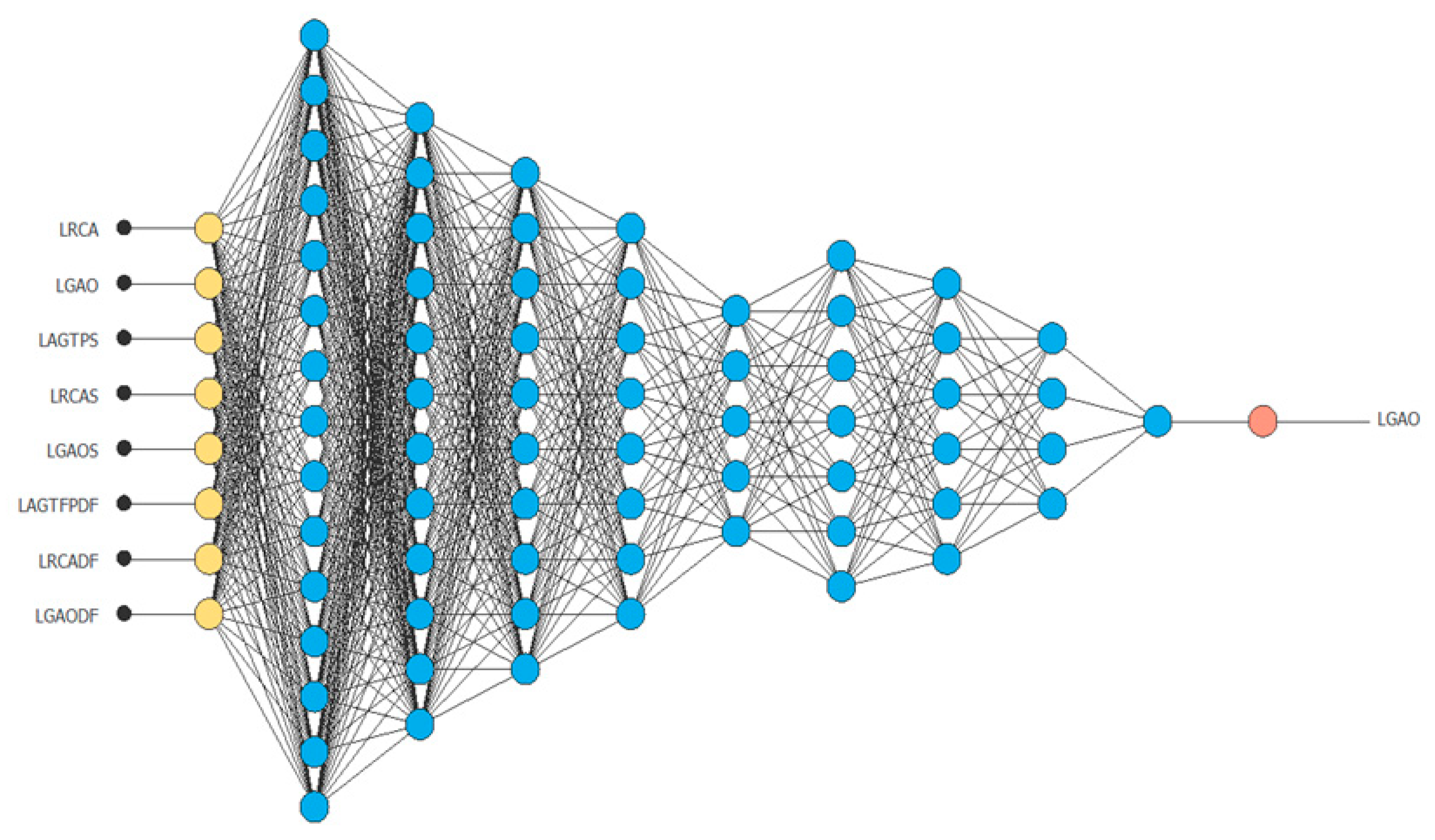
- ANNs, unlike standard econometric models and their software, do not have to be programmed to perform a task. ANNs learn independently based on experience or with the help of an external instructor. Therefore, we used the same dataset as the PVAR econometric modeling; however, we expanded the observations through the quadratic transforms (LRCAS, LAGTPS, and LGAOS) and firsts differences of each variable (LRCADF, LAGTPD,F and LRCADF). In this way, our neural network has worked on over 21,000 data and has guaranteed us a better ML results.
4. Results
5. Conclusions and Policy Implications
Supplementary Materials
Author Contributions
Funding
Informed Consent Statement
Data Availability Statement
Conflicts of Interest
Appendix A

| Abbreviation | Description | Source |
|---|---|---|
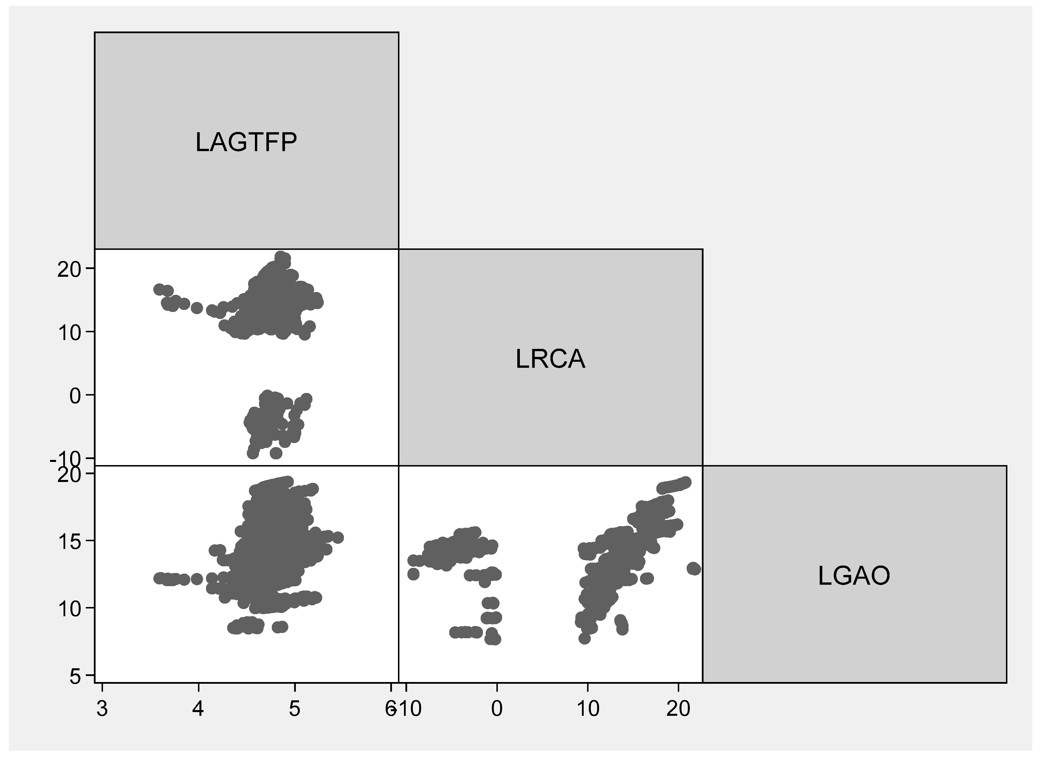
| LAGTFP | Agricultural TFP indexes (based year 1961 = 100) | WDI |
| LRCA | Credit to agriculture, USD, 2005 prices | WDI |
| LGAO | Gross agricultural output | WDI |
| Variable | Mean | Median | SD | Skewness | Kurtosis | IQR | 10-Trim | PSD |
|---|---|---|---|---|---|---|---|---|
| Full sample | ||||||||
| LAGTFP | 4.7247 | 4.6974 | 0.1878 | −0.3518 | 7.1713 | 0.2259 | 4.7190 | 0.1675 |
| LRCA | 10.8572 | 13.3334 | 7.7163 | −1.1710 | 3.0324 | 5.7287 | 11.8600 | 4.2470 |
| LGAO | 14.2442 | 14.4412 | 2.3128 | −0.4859 | 2.8906 | 2.8957 | 14.3900 | 2.1470 |
| OECD | ||||||||
| LAGTFP | 4.7539 | 4.7381 | 0.1588 | 0.2006 | 2.4794 | 0.2248 | 4.7500 | 0.1666 |
| LRCA | 18.1554 | 18.1062 | 1.3555 | 0.0825 | 1.6893 | 2.5493 | 18.1600 | 1.8900 |
| LGAO | 16.3678 | 17.0177 | 1.2610 | −1.2285 | 3.5643 | 1.4994 | 16.5800 | 1.1120 |
| Developing | ||||||||
| LAGTFP | 4.7275 | 4.6944 | 0.1753 | 0.5943 | 3.5870 | 0.2241 | 4.7160 | 0.1661 |
| LRCA | 10.1588 | 12.7988 | 7.5960 | −1.1751 | 2.9321 | 4.9499 | 11.1600 | 3.6690 |
| LGAO | 14.1416 | 14.3401 | 2.2467 | −0.3843 | 2.8372 | 2.7683 | 14.2400 | 2.0520 |
| Net Food Importing Developing | ||||||||
| LAGTFP | 4.7083 | 4.6799 | 0.1588 | 1.3461 | 5.8767 | 0.1589 | 4.6890 | 0.1178 |
| LRCA | 8.6626 | 11.6343 | 7.3240 | −0.9090 | 2.2020 | 14.2934 | 9.4100 | 10.6000 |
| LGAO | 13.3027 | 13.8673 | 2.2702 | −0.4519 | 2.2996 | 3.0951 | 2.2940 | 3.0950 |
| Least Developed | ||||||||
| LAGTFP | 4.6975 | 4.6581 | 0.1679 | 1.1617 | 5.2129 | 0.1642 | 4.6820 | 0.1217 |
| LRCA | 4.5156 | 9.9942 | 8.7194 | −0.1587 | 1.1835 | 16.9595 | 4.7180 | 12.5700 |
| LGAO | 13.8314 | 14.0033 | 1.3480 | −0.2158 | 2.5083 | 1.9594 | 13.8600 | 1.4520 |
| Variable | Groups | Mean | N | Standard Error | Standard Deviation | t | Satterthwaite’s d.o.f. | Wilcoxon Test | Kruskal–Wallis Test | One-Way ANOVA F Test | Pearson χ2 Test | Kolmogorov–Smirnov Test |
|---|---|---|---|---|---|---|---|---|---|---|---|---|
| 1. LAGTFP | Non-OECD | 4.72 | 1955 | 0.0043 | 0.1912 | −3.18 | 396.77 | −3.233 (0.0012) | 10.452 (0.0012) | 7.66 (0.0057) | 14.453 (0.000) | 0.1290 (0.001) |
| OECD | 4.75 | 276 | 0.0096 | 0.1588 | ||||||||
| 2. LAGTFP | Non-Developing | 4.70 | 276 | 0.0156 | 0.2591 | −1.43 | 311.51 | 1.753 (0.0797) | 3.072 (0.0796) | 3.64 (0.0565) | 7.689 (0.006) | 0.0959 (0.023) |
| Developing | 4.73 | 1955 | 0.0040 | 0.1753 | ||||||||
| 3. LAGTFP | Non-NFID | 4.73 | 1725 | 0.0047 | 0.1952 | 2.49 | 995.09 | 3.612 (0.0003) | 13.050 (0.0003) | 4.97 (0.0259) | 12.803 (0.000) | 0.1547 (0.000) |
| NFID | 4.71 | 506 | 0.0071 | 0.1588 | ||||||||
| 4. LAGTFP | Non-LD | 4.73 | 1679 | 0.0047 | 0.1931 | 4.21 | 1067.55 | 5.782 (0.0000) | 33.436 (0.0001) | 15.42 (0.0001) | 27.433 (0.000) | 0.1502 (0.000) |
| LD | 4.70 | 552 | 0.0071 | 0.1679 | ||||||||
| 5. LRCA | Non-OECD | 9.97 | 885 | 0.2589 | 7.7008 | −28.20 | 901.43 | −14.956 (0.0000) | 223.675 (0.0001) | 120.20 (0.0000) | 117.705 (0.000) | 0.8305 (0.000) |
| OECD | 18.16 | 107 | 0.1310 | 1.3555 | ||||||||
| 6. LRCA | Non-Developing | 14.99 | 144 | 0.5948 | 7.1382 | 7.41 | 202.02 | 11.382 (0.0000) | 129.556 (0.0001) | 50.22 (0.0000) | 79.620 (0.000) | 0.5559 (0.000) |
| Developing | 10.16 | 848 | 0.2608 | 7.5960 | ||||||||
| 7. LRCA | Non-NFID | 11.87 | 679 | 0.2950 | 7.6874 | 6.31 | 634.11 | 9.339 (0.0000) | 87.224 (0.0001) | 38.38 (0.0000) | 78.883 (0.000) | 0.3204 (0.000) |
| NFID | 8.66 | 313 | 0.4140 | 7.3240 | ||||||||
| 8. LRCA | Non-LD | 13.10 | 733 | 0.2171 | 5.8784 | 14.70 | 344.39 | 15.498 (0.0000) | 240.190 (0.0001) | 310.74 (0.0000) | 147.478 (0.000) | 0.4778 (0.000) |
| LD | 4.52 | 259 | 0.5418 | 8.7194 | ||||||||
| 9. LGAO | Non-OECD | 13.97 | 2139 | 0.0492 | 2.2755 | −26.51 | 542.34 | −17.794 (0.0000) | 316.638 (0.0001) | 294.65 (0.0000) | 214.734 (0.000) | 0.6072 (0.000) |
| OECD | 16.37 | 276 | 0.0759 | 1.2610 | ||||||||
| 10. LGAO | Non-Developing | 14.97 | 299 | 0.1520 | 2.6275 | 5.19 | 362.21 | 7.502 (0.0000) | 56.275 (0.0001) | 34.11 (0.0000) | 49.715 (0.000) | 0.3286 (0.000) |
| Developing | 14.14 | 2116 | 0.0488 | 2.2467 | ||||||||
| 11. LGAO | Non-NFID | 14.60 | 1748 | 0.0533 | 2.2269 | 12.66 | 1183.98 | 11.699 (0.0000) | 136.871 (0.0001) | 162.95 (0.0000) | 68.403 (0.000) | 0.2228 (0.000) |
| NFID | 13.30 | 667 | 0.0879 | 2.2702 | ||||||||
| 12. LGAO | Non-LD | 14.37 | 1863 | 0.0583 | 2.5163 | 6.54 | 1730.31 | 7.772 (0.0000) | 60.401 (0.0001) | 23.00 (0.0000) | 80.174 (0.000) | 0.2869 (0.000) |
| LD | 13.83 | 552 | 0.0574 | 1.3480 |

References
- Azariadis, C.; Drazen, A. Threshold externalities in economic development. Q. J. Econ. 1990, 105, 501–526. [Google Scholar] [CrossRef]
- Besley, T. How do market failures justify interventions in rural credit markets? World Bank Res. Obs. 1994, 9, 27–47. [Google Scholar] [CrossRef] [Green Version]
- Karlan, D.; Morduch, J. Access to finance. In Handbook of Development Economics; Elsevier: Amsterdam, The Netherlands, 2010; Volume 5, pp. 4703–4784. [Google Scholar]
- Levine, R. Finance and growth: Theory and evidence. In Handbook of Economic Growth; Elsevier: Amsterdam, The Netherlands, 2005; Volume 1, pp. 865–934. [Google Scholar]
- Rajan, R.G.; Zingales, L. Financial dependence and growth. Am. Econ. Rev. 1998, 88, 559–586. [Google Scholar]
- Beck, T.; Levine, R.; Loayza, N. Finance and the sources of growth. J. Financ. Econ. 2000, 58, 261–300. [Google Scholar] [CrossRef] [Green Version]
- Levine, R.; Loayza, N.; Beck, T. Financial intermediation and growth: Causality and causes. J. Monet. Econ. 2000, 46, 31–77. [Google Scholar] [CrossRef] [Green Version]
- Winter-Nelson, A.; Temu, A.A. Liquidity constraints, access to credit and pro-poor growth in rural Tanzania. J. Int. Dev. 2005, 17, 867–882. [Google Scholar] [CrossRef]
- Zang, H.; Kim, Y.C. Does financial development precede growth? Robinson and Lucas might be right. Appl. Econ. Lett. 2007, 14, 15–19. [Google Scholar] [CrossRef]
- Baliamoune-Lutz, M. Financial Development and Income in African Countries. Contemp. Econ. Policy 2013, 31, 163–175. [Google Scholar] [CrossRef]
- Feder, G.; Lau, L.J.; Lin, J.Y.; Luo, X. The relationship between credit and productivity in Chinese agriculture: A microeconomic model of disequilibrium. Am. J. Agric. Econ. 1990, 72, 1151–1157. [Google Scholar] [CrossRef]
- Rozelle, S.; Taylor, J.E.; DeBrauw, A. Migration, remittances, and agricultural productivity in China. Am. Econ. Rev. 1999, 89, 287–291. [Google Scholar] [CrossRef]
- Foltz, J.D. Credit market access and profitability in Tunisian agriculture. Agric. Econ. 2004, 30, 229–240. [Google Scholar] [CrossRef]
- O’Toole, C.M.; Newman, C.; Hennessy, T. Financing constraints and agricultural investment: Effects of the Irish financial crisis. J. Agric. Econ. 2014, 65, 152–176. [Google Scholar] [CrossRef]
- Zhang, T.; Liu, H.; Liang, P. Social Trust Formation and Credit Accessibility—Evidence from Rural Households in China. Sustainability 2020, 12, 667. [Google Scholar] [CrossRef] [Green Version]
- Linh, T.N.; Long, H.T.; Chi, L.V.; Tam, L.T.; Lebailly, P. Access to rural credit markets in developing countries, the case of Vietnam: A literature review. Sustainability 2019, 11, 1468. [Google Scholar] [CrossRef] [Green Version]
- Moahid, M.; Maharjan, K.L. Factors Affecting Farmers’ Access to Formal and Informal Credit: Evidence from Rural Afghanistan. Sustainability 2020, 12, 1268. [Google Scholar] [CrossRef] [Green Version]
- Liu, J.; Wang, M.; Yang, L.; Rahman, S.; Sriboonchitta, S. Agricultural Productivity Growth and Its Determinants in South and Southeast Asian Countries. Sustainability 2020, 12, 4981. [Google Scholar] [CrossRef]
- Niu, Z.; Yan, H.; Liu, F. Decreasing Cropping Intensity Dominated the Negative Trend of Cropland Productivity in Southern China in 2000–2015. Sustainability 2020, 12, 10070. [Google Scholar] [CrossRef]
- Sadeh, A.; Radu, C.F.; Feniser, C.; Borşa, A. Governmental Intervention and Its Impact on Growth, Economic Development, and Technology in OECD Countries. Sustainability 2021, 13, 166. [Google Scholar] [CrossRef]
- Guirkinger, C.; Boucher, S.R. Credit constraints and productivity in Peruvian agriculture. Agric. Econ. 2008, 39, 295–308. [Google Scholar] [CrossRef]
- Dong, F.; Lu, J.; Featherstone, A.M. Effects of credit constraints on household productivity in rural China. Agric. Financ. Rev. 2012, 72, 402–415. [Google Scholar] [CrossRef]
- Ali, D.A.; Deininger, K.; Duponchel, M. Credit Constraints, Agricultural Productivity, and Rural Nonfarm Participation: Evidence from Rwanda; The World Bank: Washington, DC, USA, 2014. [Google Scholar]
- Petrick, M. Farm investment, credit rationing, and governmentally promoted credit access in Poland: A cross-sectional analysis. Food Policy 2004, 29, 275–294. [Google Scholar] [CrossRef]
- King, R.G.; Levine, R. Finance and growth: Schumpeter might be right. Q. J. Econ. 1993, 108, 717–738. [Google Scholar] [CrossRef]
- Hartarska, V.; Nadolnyak, D.; Shen, X. Agricultural credit and economic growth in rural areas. Agric. Financ. Rev. 2015, 75, 302–312. [Google Scholar] [CrossRef]
- Rehman, A.; Chandio, A.A.; Hussain, I.; Jingdong, L. Is credit the devil in the agriculture? The role of credit in Pakistan’s agricultural sector. J. Financ. Data Sci. 2017, 3, 38–44. [Google Scholar] [CrossRef]
- Kochar, A. An empirical investigation of rationing constraints in rural credit markets in India. J. Dev. Econ. 1997, 53, 339–371. [Google Scholar] [CrossRef]
- Schumpeter, J.A. The Theory of Economic Development; Harvard University Press: Cambridge, MA, USA, 1911. [Google Scholar]
- Patrick, H.T. Financial development and economic growth in underdeveloped countries. Econ. Dev. Cult. Chang. 1966, 14, 174–189. [Google Scholar] [CrossRef]
- McKinnon, R.I. Money and Capital in Economic Development; The Brookings Institute: Washington, DC, USA, 1973. [Google Scholar]
- Shaw, E.S. Financial Deepening in Economic Development; Oxford University Press: New York, NY, USA, 1973. [Google Scholar]
- De Gregorio, J.; Guidotti, P.E. Financial development and economic growth. World Dev. 1995, 23, 433–448. [Google Scholar] [CrossRef]
- Levine, R.; Zervos, S. Stock market development and long-run growth. World Econ. Rev. 1996, 110, 323–340. [Google Scholar] [CrossRef] [Green Version]
- Yang, Y.Y.; Yi, M.H. Does financial development cause economic growth? Implication for policy in Korea. J. Policy Model. 2008, 30, 827–840. [Google Scholar] [CrossRef]
- Greenwood, J.; Jovanovic, B. Financial development, growth, and the distribution of income. J. Political Econ. 1990, 98, 1076–1107. [Google Scholar] [CrossRef] [Green Version]
- Bencivenga, V.R.; Smith, B.D. Financial intermediation and endogenous growth. Rev. Econ. Stud. 1991, 58, 195–209. [Google Scholar] [CrossRef]
- Roubini, N.; Sala-i Martin, X. Financial repression and economic growth. J. Dev. Econ. 1992, 39, 5–30. [Google Scholar] [CrossRef] [Green Version]
- Diallo, B.; Al-Titi, O. Local growth and access to credit: Theory and evidence. J. Macroecon. 2017, 54, 410–423. [Google Scholar] [CrossRef]
- Robinson, J. The Rate of Interest and Other Essays; MacMillan: London, UK, 1952. [Google Scholar]
- Lucas, R.E., Jr. On the mechanics of economic development. J. Monet. Econ. 1988, 22, 3–42. [Google Scholar] [CrossRef]
- Stern, N. The economics of development: A survey. Econ. J. 1989, 100, 597–685. [Google Scholar] [CrossRef]
- Chandavarkar, A. Of finance and development: Neglected and unsettled questions. World Dev. 1992, 22, 133–142. [Google Scholar] [CrossRef]
- Stiglitz, J. The role of the state in financial markets. In Proceedings of the World Bank Conference on Development Economics, Washington, DC, USA, 28–29 April 1994; Bruno, M., Pleskovic, B., Eds.; World Bank: Washington, DC, USA, 1994. [Google Scholar]
- Gurley, J.; Shaw, E. Financial structure and economic development. Econ. Dev. Cult. Chang. 1967, 34, 333–346. [Google Scholar] [CrossRef]
- Goldsmith, R.W. Financial Structure and Development; National Bureau of Economic Research: New Haven, CT, USA, 1969. [Google Scholar]
- Demetriades, P.O.; Hussein, K.A. Does financial development cause economic growth? Time-series evidence from 16 countries. J. Dev. Econ. 1996, 51, 387–411. [Google Scholar] [CrossRef]
- Luintel, K.B.; Khan, M. A Quantitative Reassessment of the Finance-Growth Nexus: Evidence from a Multivariate VAR. J. Dev. Econ. 1999, 60, 381–405. [Google Scholar] [CrossRef]
- Calderón, C.; Liu, L. The Direction of Causality between Financial Development and Economic Growth. J. Dev. Econ. 2003, 72, 321–334. [Google Scholar] [CrossRef] [Green Version]
- Kar, M.; Nazlıoğlu, S.; Ağır, H. Financial development and economic growth nexus in the MENA countries: Bootstrap panel granger causality analysis. Econ. Model. 2011, 28, 685–693. [Google Scholar] [CrossRef]
- Neusser, K.; Kugler, M. Manufacturing growth and financial development: Evidence from OECD countries. Rev. Econ. Stat. 1998, 80, 638–646. [Google Scholar] [CrossRef]
- Rousseau, P.L.; Wachtel, P. Equity markets and growth: Cross-country evidence on timing and outcomes, 1980–1995. J. Bank. Financ. 2000, 24, 1933–1957. [Google Scholar] [CrossRef]
- Magazzino, C. GDP, Energy Consumption and Financial Development in Italy. Int. J. Energy Sect. Manag. 2018, 12, 28–43. [Google Scholar] [CrossRef] [Green Version]
- Demetriades, P.O.; Luintel, K.B. Banking Sector Policies and Financial Development in Nepal. Oxf. Bull. Econ. Stat. 1996, 58, 355–372. [Google Scholar] [CrossRef]
- Beck, T.; Demirgüç-Kunt, A. Access to Finance: An Unfinished Agenda. World Bank Econ. Rev. 2008, 22, 383–396. [Google Scholar] [CrossRef] [Green Version]
- Love, I.; Martínez Pería, M.S. How Bank Competition Affects Firms’ Access to Finance. World Bank Econ. Rev. 2014, 29, 413–448. [Google Scholar] [CrossRef] [Green Version]
- Ayyagari, M.; Demirgüç-Kunt, A.; Maksimovic, V. How Important Are Financing Constraints? The Role of Finance in the Business Environment. World Bank Econ. Rev. 2008, 22, 483–516. [Google Scholar] [CrossRef]
- Magazzino, C.; Mele, M.; Morelli, G. The relationship between renewable energy and economic growth in a time of Covid-19: A Machine Learning experiment on the Brazilian economy. Sustainability 2021, 13, 1285. [Google Scholar] [CrossRef]
- Magazzino, C.; Mele, M.; Sarkodie, S.A. The nexus between COVID-19 deaths, air pollution and economic growth in New York state: Evidence from Deep Machine Learning. J. Environ. Manage. 2021, 286, 112241. [Google Scholar] [CrossRef]
- Magazzino, C.; Mele, M.; Schneider, N. A D2C Algorithm on the Natural Gas Consumption and Economic Growth: Challenges faced by Germany and Japan. Energy 2021, 219, 19586. [Google Scholar] [CrossRef]
- Magazzino, C.; Mele, M.; Schneider, N. A Machine Learning approach on the relationship among solar and wind energy production, coal consumption, GDP, and CO2 emissions. Renew. Energy 2021, 167, 99–115. [Google Scholar] [CrossRef]
- Magazzino, C.; Mele, M.; Schneider, N. The relationship between air pollution and COVID-19-related deaths: An application to three French cities. Appl. Energy 2020, 279. [Google Scholar]
- Magazzino, C.; Mele, M.; Schneider, N. The relationship between municipal solid waste and greenhouse gas emissions: Evidence from Switzerland. Waste Manag. 2020, 113, 508–520. [Google Scholar] [CrossRef] [PubMed]
- Magazzino, C.; Mele, M.; Schneider, N.; Sarkodie, S.A. Waste generation, Wealth and GHG emissions from the waste sector: Is Denmark on the path towards Circular Economy? Sci Total Environ. 2021, 755, 142510. [Google Scholar] [CrossRef]
- Magazzino, C.; Mele, M.; Schneider, N.; Vallet, G. The Relationship between Nuclear Energy Consumption and Economic Growth: Evidence from Switzerland. Environ. Res. Lett. 2020, 15, 0940a5. [Google Scholar] [CrossRef]
- Mele, M.; Magazzino, C. A Machine Learning Analysis of the Relationship among Iron and Steel Industries, Air Pollution, and Economic Growth in China. J. Clean. Prod. 2020, 277, 123293. [Google Scholar] [CrossRef]
- Mele, M.; Magazzino, C.; Schneider, N.; Strezov, V. NO2 levels as a contributing factor to COVID-19 deaths: The first empirical estimate of threshold values. Environ. Res. 2021, 194, 110663. [Google Scholar] [CrossRef] [PubMed]
- Mele, M.; Magazzino, C. Pollution, Economic Growth and COVID-19 Deaths in India: A Machine Learning Evidence. Environ Sci Pollut Res Int. 2021, 28, 2669–2677. [Google Scholar] [CrossRef] [PubMed]
- Bai, L.; Boudot, C.; Butler, A.; Eigner, J. Rural Banks and Agricultural Production: Evidence from India’s Social Banking Experiment. Work. Pap. 2018. [Google Scholar]
- Verdoorn, P.J. Fattori che regolano lo sviluppo della produttività del lavoro. L’Industria 1949, 1, 3–10. [Google Scholar]
- Foster, A.D.; Rosenzweig, M.R. Learning by doing and learning from others: Human capital and technical change in agriculture. J. Political Econ. 1995, 103, 1176–1209. [Google Scholar] [CrossRef]
- Conley, T.G.; Udry, C.R. Learning about a new technology: Pineapple in Ghana. Am. Econ. Rev. 2010, 100, 35–69. [Google Scholar] [CrossRef] [Green Version]
- Bardhan, P.; Udry, C. Development Microeconomics; OUP: Oxford, UK, 1999. [Google Scholar]


| Author(s) | Country | Study Period | Empirical Strategy | Direction of Relationships |
|---|---|---|---|---|
| Rozelle et al. (1999) | China | 1995 | Cross section | CA → P |
| Feder et al. (1990) | China | 1987 | Cross section | CA → P |
| Foltz (2004) | Tunisia | 1995 | Cross section | CA → P |
| Kochar (1997) | India | 1981–1982 | Cross section | |
| Petrick (2004) | Poland | 2000 | Cross section | |
| O’Toole et al. (2014) | Ireland | 1997–2010 | Panel data | |
| Guirkinger and Boucher (2008) | Peru | 1997 and 2003 | Panel data | CA → P |
| Ali et al. (2014) | Rwanda | 2011 | Cross section | CA → P |
| Hartarska et al. (2015) | USA | 1991–2010 | Panel data | |
| Dong et al. (2012) | China | 2008 | Cross section | CA → P |
| Rehman et al. (2017) | Pakistan | 1960–2015 | Time series |
| Author(s) | Country | Study Period | Empirical Strategy | Direction of Relationships |
|---|---|---|---|---|
| King and Levine (1993) | 80 countries | 1960–1989 | Cross-country regressions | FD → EC |
| De Gregorio and Guidotti (1995) | 80 countries | 1960–1985 | Cross-country regressions | FD → EC |
| Demetriades and Hussein (1996) | 16 countries | 1960–1993 | Time series | FD ↔ EC |
| Demetriades and Luintel (1996) | Nepal | 1960–1992 | Time series | FD ↔ EC |
| Levine and Zervos (1996) | 41 countries | 1976–1993 | Cross-country regressions | FD → EC |
| Neusser and Kugler (1998) | 13 countries | 1970–1991 | Time series | FD → EC |
| Rajan and Zingales (1998) | 55 countries | 1980–1990 | Cross-country regressions | FD → EC |
| Luintel and Khan (1999) | 10 countries | Time series | FD ↔ EC | |
| Beck et al. (2000) | 63 countries | 1960–1995 | Cross-country and panel data | FD → EC |
| Levine et al. (2000) | 74 countries | 1960–1995 | Cross-country and panel data | FD → EC |
| Rousseau and Wachtel (2000) | 47 countries | 1980–1995 | Panel data | FD → EC |
| Calderón and Liu (2003) | 109 countries | 1960–1994 | Geweke decomposition test on pooled data | FD ↔ EC |
| Yang and Yi (2008) | Korea | 1971–2002 | Time series | FD → EC |
| Zang and Kim (2007) | 74 countries | 1961–1995 | Panel data | FD ← EC |
| Kar et al. (2011) | MENA countries | 1980–2007 | Panel data | Mixed results |
| Baliamoune-Lutz (2013) | 18 African countries | 1960–2001 | Time series | FD ↔ EC |
| Magazzino (2018) | Italy | 1960-2014 | Time series | FD → EC |
| Predicted Positive | Predicted Negative | |
|---|---|---|
| Actual Positive | 20,043 | 128 |
| Actual Negative | 143 | 20,020 |
| Accuracy | 0.993 | |
| Precision | 0.992 | |
| Sensitivity | 0.993 | |
| SP | 0.992 | |
| FPR | 0.007 | |
| Predicted Positive | Predicted Negative | |
|---|---|---|
| Actual Positive | 19,852 | 319 |
| Actual Negative | 712 | 19,451 |
| Accuracy | 0.974 | |
| Precision | 0.956 | |
| Sensitivity | 0.984 | |
| SP | 0.964 | |
| FPR | 0.035 | |
Publisher’s Note: MDPI stays neutral with regard to jurisdictional claims in published maps and institutional affiliations. |
© 2021 by the authors. Licensee MDPI, Basel, Switzerland. This article is an open access article distributed under the terms and conditions of the Creative Commons Attribution (CC BY) license (http://creativecommons.org/licenses/by/4.0/).
Share and Cite
Magazzino, C.; Mele, M.; Santeramo, F.G. Using an Artificial Neural Networks Experiment to Assess the Links among Financial Development and Growth in Agriculture. Sustainability 2021, 13, 2828. https://doi.org/10.3390/su13052828
Magazzino C, Mele M, Santeramo FG. Using an Artificial Neural Networks Experiment to Assess the Links among Financial Development and Growth in Agriculture. Sustainability. 2021; 13(5):2828. https://doi.org/10.3390/su13052828
Chicago/Turabian StyleMagazzino, Cosimo, Marco Mele, and Fabio Gaetano Santeramo. 2021. "Using an Artificial Neural Networks Experiment to Assess the Links among Financial Development and Growth in Agriculture" Sustainability 13, no. 5: 2828. https://doi.org/10.3390/su13052828